Molecular Feshbach dissociation as a source for motionally entangled atoms

Abstract

We describe the dissociation of a diatomic Feshbach molecule due to a time-varying external magnetic field in a realistic trap and guide setting. An analytic expression for the asymptotic state of the two ultracold atoms is derived, which can serve as a basis for the analysis of dissociation protocols to generate motionally entangled states. For instance, the gradual dissociation by sequences of magnetic field pulses may delocalize the atoms into macroscopically distinct wave packets, whose motional entanglement can be addressed interferometrically. The established relation between the applied magnetic field pulse and the generated dissociation state reveals that square-shaped magnetic field pulses minimize the momentum spread of the atoms. This is required to control the detrimental influence of dispersion in a recently proposed experiment to perform a Bell test in the motion of the two atoms [C. Gneiting and K. Hornberger, Phys. Rev. Lett. 101, 260503 (2008)].

I Introduction

The emerging field of ultracold atoms makes it possible to perform hitherto unprecedented experiments on the quantum nature of material objects, thus introducing a new quality compared to previous quantum experiments with immaterial photons. This is owing to the experimental control over the atomic state reaching a level where quantum mechanical effects become relevant. Given that Bose-Einstein condensates (BECs) are nowadays routinely produced, they can serve as an ideal starting point, for example, to probe condensed matter physics in a highly controlled environment provided by optical lattices Bloch2008a ; Buchleitner2003a ; witthaut:200402 ; hartung:020603 . A considerable extension of the scope of such experiments has been achieved by exploiting Feshbach resonances to produce molecules and molecular BECs (mBECs) Cubizolles2003a ; Jochim2003a ; Regal2003a ; Greiner2003a ; Strecker2003a ; Herbig2003a ; Xu2003a ; Durr2004a . The ability to control the interaction between the atoms with an external magnetic field permits one to realize, for example, the BCS-BEC crossover Bloch2008a or Efimov states Kraemer2006a , and to establish coherent atom-molecule oscillations Donley2002a ; Claussen2003a ; Borca2003a ; Duine2004a ; Goral2005a , hinting at quantum-coherent chemistry.

Beyond that, it has been recognized that the controlled dissociation of mBECs can also serve as a resource for entangled atom pairs that would permit the demonstration of nonclassical correlations on a macroscopic level Kheruntsyan2005a ; Kheruntsyan2006a . The use of such a controlled dissociation for spectroscopic purposes has already been discussed theoretically Durr2005z ; Hanna2006a and demonstrated experimentally Mukaiyama2004a ; Durr2004b . In a recent proposal, we investigated the possibility of using an arranged dissociation of Feshbach molecules in order to violate a Bell inequality in the motion of two atoms Gneiting2008a . There, a sequence of two short magnetic field pulses dissociates a single molecule out of a dilute mBEC such that each atom is delocalized into two macroscopically distinct wave packets propagating along the laser guide. The associated dissociation-time entangled (DTE) state can be considered the matter wave analog of a Bell state Gneiting2009a , whose capability to yield nonclassical correlations can be revealed by an interferometric protocol reuniting the wave packets on each side Brendel1999a ; Tittel2000a . The violation of a Bell inequality, however, imposes stringent requirements on the DTE state, which makes it necessary to know the generated dissociation state in detail Gneiting2009a .

The theory of Feshbach molecules is mainly concerned with an accurate description of the molecules in the bound regime and its vicinity, where the atoms interact strongly. For instance, it has been investigated in great detail that the molecular state at constant magnetic field exhibits universal properties in the vicinity of a Feshbach resonance, as well as the association and dissociation behaviors under a linear magnetic field sweep, with emphasis on the converted fraction (see Hanna2006a ; Kohler2006a ; Nygaard2008a and Refs. therein). An appropriate description of the situation proposed in Gneiting2008a , however, requires a detailed knowledge of the dissociation state for a more general temporal behavior of the magnetic field, varying on short time scales compared to the inverse resonance width. While in the interaction regime of the atoms one is then forced to resort to numerical methods Mies2000a , the restriction to the asymptotic situation (i.e. for large interatomic distances and times long after the dissociation process) comes with significant simplifications that permit one to evaluate the generated dissociation state analytically.

In this article we present a coupled-channels formulation of the dissociation process of an initially trapped Feshbach molecule exposed to a time-varying homogeneous magnetic field. These single-molecule dynamics yield an adequate description in the relevant case of the dissociation of a single molecule out of a dilute mBEC, where interactions between the molecules and statistical effects do not play a role. The formulation includes the center of mass motion required for the complete description of the two-particle system. The dissociation is considered to take place in a shallow trap from where the dissociated atoms are injected into a strong guiding potential, which confines them to the longitudinal motion along the guide axis. Based on the time-dependent coupled-channel equations, we derive an analytic expression for the asymptotic dissociation state of the ultracold atoms, allowing us to investigate the relation between the form of the applied magnetic field pulse and the resulting two-particle dissociation state. While Gaussian-shaped dissociation pulses turn out to yield a rather bulky momentum distribution of the two-particle state, we demonstrate that idealized square-shaped magnetic field pulses optimize the momentum distribution with respect to its sharpness.

The structure of this article is as follows. In Section II we describe the assumed geometry of trap and guiding potentials, which is the natural configuration for dissociation experiments. The time-dependent coupled-channel equations are formulated in Section III, and then reduced to an integro-differential equation for the closed-channel amplitude and an associated equation for the background channel state. Section IV shows how the asymptotic dissociation state can be expressed in terms of the Fourier transform of the closed-channel amplitude. The approximate dynamics of the latter for a given shape of the magnetic field pulse is described in Section V; this allows us, in Section VI, to discuss the optimal form of the pulse if a narrow momentum distribution of the dissociation products is required, such as for the test of the Bell inequality proposed in Gneiting2008a . Applications of the Feshbach dissociation scheme as a resource of entangled atom states beyond the scenario in Gneiting2008a are discussed in the Conclusions.

II Trap and guide configuration

Before presenting the coupled-channels formalism, we outline an experimental setup that meets the conditions assumed in our dissociation scenario. An explicit quantitative elaboration was given in Gneiting2009b .

Consider a BEC of Feshbach molecules in an optical dipole trap, which can be established by two perpendicularly crossing laser beams, see Figure 1 a). The weak trap laser guarantees longitudinal confinement within the wave guide produced by the strong guiding laser. We take the BEC, of the order of $10^{2}$ molecules, to be sufficiently dilute such that one may neglect interactions between different molecules. This may be accomplished by choosing a mBEC of fermionic constituents, for example ${}^{6}\operatorname{Li}_{2}$, where Pauli blocking further reduces the effect of intermolecular interactions and thus enhances the lifetime of the mBEC Jochim2003aORIG .

The molecules can then be considered to be in a product state with the center of mass motion given by the ground state of the trap, whereas the relative motion is in a bound molecular state. The latter can be turned into a Feshbach resonance by varying the external magnetic field, allowing one to dissociate the atoms in a controlled way. By applying one or several appropriately chosen dissociation pulses, a single molecule dissociates into two counter-propagating atoms on average, and we postselect the single-dissociation events.

The pulses provide the atoms with a kinetic energy sufficiently large to overcome the trap potential in longitudinal direction, but still below the threshold to get beyond the ground state transversally, see Figure 1 b). This way we may end up with two dissociated atoms, counter-propagating with a velocity on the order of 1 cm/s along the guiding laser axis, whose two-particle state is determined by the initial state of the molecule and the dissociation pulse shape. By applying sequences of dissociation pulses, one can design highly nonclassical, motionally entangled states that can further be processed for various fundamental tests of quantum mechanics, such as to violate a Bell inequality Gneiting2008a .

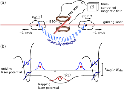
Figure 1: (color online) a) Setup for generating pairs of motionally entangled atoms by the Feshbach dissociation of molecules. Initially, a BEC of on the order of $10^{2}$ Feshbach molecules resides in a dipole trap produced by two crossing laser beams. An externally controlled, homogeneous magnetic field induces the dissociation of one molecule per trial and thus generates a pair of atoms moving along the laser guide at a velocity on the order of 1 cm/s. The asymptotic two-atom state in the wave guide is determined by the trap and guide geometry and by the shape of the dissociation pulse. b) The dissociation pulse promotes the trapped molecule to a pair of counter-propagating atoms. The laser parameters are chosen such that the energy supply from the magnetic field sweep exceeds the trap laser potential, while it cannot lead to an additional transversal excitation if the kinetic energy of the atoms $E_{\text{kin}}$ remains below the harmonic energy gap, $\hbar\omega_{\text{G}}>E_{\operatorname{kin}}$.

III coupled-channels formulation

The dynamics of Feshbach molecules is appropriately described by the coupled channels formulation. In our case, the channels are characterized by different nuclear spin configurations of the two-atom system. The different magnetic field dependences of the corresponding energy levels make it possible to manipulate the system externally. In the following we adopt the notation and the conventions from Kohler2006a as far as possible. As a novelty, we must include also the center of mass motion of the two atoms. We assume that the magnetic field remains always in the vicinity of a single Feshbach resonance, allowing us to restrict the description to two channels: the closed channel of the energetically more favorable spin configuration supporting the molecular bound state, and the background channel, where the dissociated atoms are asymptotically free.

III.1 Hamiltonian and coupled-channel equations

The two-channel Hamiltonian for the two atoms (here taken to be of equal mass $m$) can be written as

$$H_{\operatorname{tot}} = H_{\operatorname{cl}}|\operatorname{cl}\rangle\langle\operatorname{cl}|+H_{\operatorname{bg}}|\operatorname{bg}\rangle\langle\operatorname{bg}|$$ (1)

$$+W|\operatorname{bg}\rangle\langle\operatorname{cl}|+W^{\dagger}|\operatorname{cl}\rangle\langle\operatorname{bg}|,$$

with the closed-channel Hamiltonian

$$H_{\operatorname{cl}} = -\frac{\hbar^{2}}{2m}\nabla_{1}^{2}-\frac{\hbar^{2}}{2m}\nabla^{2}_{2}+V_{\operatorname{cl}}(|\boldsymbol{x}_{1}-\boldsymbol{x}_{2}|,B(t))$$ (2)

$$+V_{\text{T}}(\boldsymbol{x}_{1})+V_{\text{T}}(\boldsymbol{x}_{2})+V_{\text{G}}(\boldsymbol{x}_{1})+V_{\text{G}}(\boldsymbol{x}_{2})$$

and the background (open) channel Hamiltonian

$$H_{\operatorname{bg}} = -\frac{\hbar^{2}}{2m}\nabla_{1}^{2}-\frac{\hbar^{2}}{2m}\nabla^{2}_{2}+V_{\operatorname{bg}}(|\boldsymbol{x}_{1}-\boldsymbol{x}_{2}|)$$ (3)

$$+V_{\text{T}}(\boldsymbol{x}_{1})+V_{\text{T}}(\boldsymbol{x}_{2})+V_{\text{G}}(\boldsymbol{x}_{1})+V_{\text{G}}(\boldsymbol{x}_{2}).$$

Here $V_{\text{T}}(\boldsymbol{x}_{i})$ and $V_{\text{G}}(\boldsymbol{x}_{i})$ denote the trapping and guiding laser potential, respectively ($V_{\text{G}}$ may contain a linear shift due to the gravitational potential). $V_{\operatorname{cl}}(|\boldsymbol{x}_{1}-\boldsymbol{x}_{2}|,B(t))$ and $V_{\operatorname{bg}}(|\boldsymbol{x}_{1}-\boldsymbol{x}_{2}|)$, on the other hand, describe the interatomic potentials for each channel. In general, these potentials differ for the different channels, reflecting their dependence on the spin configuration. In the chosen convention, the zero of total energy is defined in absence of the laser potentials by the background channel dissociation threshold with the center of mass at rest. Then only the closed-channel potential $V_{\operatorname{cl}}(|\boldsymbol{x}_{1}-\boldsymbol{x}_{2}|,B(t))$ depends on the external magnetic field $B(t)$, describing an overall shift with respect to the background channel dissociation threshold.

The off-diagonal elements $W$ denote the energies associated with the spin exchange interaction and provide the inter-channel coupling. We assume $W$ to be diagonal in position (i.e. independent of momentum) and to depend only on the interatomic distance $|\boldsymbol{x}_{1}-\boldsymbol{x}_{2}|$ from now on. For the following it is useful to reformulate the Hamiltonian in center of mass (cm) and relative (rel) coordinates, $\boldsymbol{x}_{\operatorname{cm}}=(\boldsymbol{x}_{1}+\boldsymbol{x}_{2})/2$ and $\boldsymbol{x}_{\operatorname{rel}}=\boldsymbol{x}_{1}-\boldsymbol{x}_{2}$, respectively, with total mass $M=2m$ and reduced mass $\mu=m/2$. The closed-channel Hamiltonian thus reads as

$$H_{\operatorname{cl}} = -\frac{\hbar^{2}}{2M}\nabla^{2}_{\operatorname{cm}}-\frac{\hbar^{2}}{2\mu}\nabla^{2}_{\operatorname{rel}}+V_{\operatorname{cl}}(|\boldsymbol{x}_{\operatorname{rel}}|,B(t))$$

$$+V_{\text{T}}(\boldsymbol{x}_{\operatorname{cm}}+\boldsymbol{x}_{\operatorname{rel}}/2)+V_{\text{T}}(\boldsymbol{x}_{\operatorname{cm}}-\boldsymbol{x}_{\operatorname{rel}}/2)$$

$$+V_{\text{G}}(\boldsymbol{x}_{\operatorname{cm}}+\boldsymbol{x}_{\operatorname{rel}}/2)+V_{\text{G}}(\boldsymbol{x}_{\operatorname{cm}}-\boldsymbol{x}_{\operatorname{rel}}/2),$$

and similar for $H_{\text{bg}}$ with $V_{\operatorname{cl}}(|\boldsymbol{x}_{\operatorname{rel}}|,B(t))$ replaced by $V_{\operatorname{bg}}(|\boldsymbol{x}_{\operatorname{rel}}|)$. Note that the center of mass motion is only indirectly affected by the homogeneous external magnetic field $B$, due to the presence of the trapping potentials. Writing

$$|\Psi_{\operatorname{tot}}(t)\rangle=\Phi_{\operatorname{cl}}(\boldsymbol{x}_{\operatorname{cm}},\boldsymbol{x}_{\operatorname{rel}},t)|\operatorname{cl}\rangle+\Phi_{\operatorname{bg}}(\boldsymbol{x}_{\operatorname{cm}},\boldsymbol{x}_{\operatorname{rel}},t)|\operatorname{bg}\rangle,$$ (5)

we can infer from the time-dependent Schrödinger equation the coupled channel equations

$$i\hbar|\Phi_{\operatorname{cl}}(t)\rangle = H_{\operatorname{cl}}(B(t))|\Phi_{\operatorname{cl}}(t)\rangle+W|\Phi_{\operatorname{bg}}(t)\rangle$$ (6)

$$i\hbar|\Phi_{\operatorname{bg}}(t)\rangle = H_{\operatorname{bg}}|\Phi_{\operatorname{bg}}(t)\rangle+W|\Phi_{\operatorname{cl}}(t)\rangle.$$

The closed channel and background channel two-particle state components $|\Phi_{\operatorname{cl}}(t)\rangle$ and $|\Phi_{\operatorname{bg}}(t)\rangle$ are thus not normalized in general. It is reasonable to assume the transverse motion of the atoms to be constrained to the region of validity of the harmonic approximation of the guiding laser potential, and the harmonic approximation to be applicable also for the trap laser potential in the closed channel. We then can write (adopting cylindrical coordinates)

$$V_{\text{G}}(\boldsymbol{x}_{1})+V_{\text{G}}(\boldsymbol{x}_{2}) = -U_{0,\text{G}}+\frac{m}{2}\omega^{2}_{\text{G}}\rho^{2}_{1}-U_{0,\text{G}}+\frac{m}{2}\omega^{2}_{\text{G}}\rho^{2}_{2}$$

$$V_{\text{T}}(\boldsymbol{x}_{1})+V_{\text{T}}(\boldsymbol{x}_{2}) = -U_{0,\text{T}}+\frac{m}{2}\omega^{2}_{\text{T}}z^{2}_{1}-U_{0,\text{T}}+\frac{m}{2}\omega^{2}_{\text{T}}z^{2}_{2}.$$

The harmonic approximation comes with the virtue not to couple the center of mass and relative motion,

$$V_{\text{G}}(\boldsymbol{x}_{1})+V_{\text{G}}(\boldsymbol{x}_{2}) = -2\,U_{0,\text{G}}+\frac{M}{2}\omega^{2}_{\text{G}}\rho^{2}_{\operatorname{cm}}+\frac{\mu}{2}\omega^{2}_{\text{G}}\rho^{2}_{\operatorname{rel}}$$

$$V_{\text{T}}(\boldsymbol{x}_{1})+V_{\text{T}}(\boldsymbol{x}_{2}) = -2\,U_{0,\text{T}}+\frac{M}{2}\omega^{2}_{\text{T}}z^{2}_{\operatorname{cm}}+\frac{\mu}{2}\omega^{2}_{\text{T}}z^{2}_{\text{rel}}.$$

The initial bound state can therefore be taken to be separable with respect to its center of mass and relative motion. Of course, the harmonic approximation for the trap laser potential breaks down when the dissociated atoms leave the trap. Then, the center of mass motion ceases to be bound by the trap potential but rather undergoes a free propagation resulting in a dispersive broadening on the spot. So, even though initially only the relative motion is affected by the external magnetic field, its effective coupling in the background channel to the center of mass also couples the motion of the latter indirectly to the external magnetic field.

III.2 Single-resonance approximation

It is legitimate Kohler2006a to take the relative motion of the closed channel state component to be proportional to the underlying bare resonance state $|\phi_{\operatorname{res}}\rangle$, which is defined by

$$\left[-\frac{\hbar^{2}}{2\mu}\nabla_{\operatorname{rel}}^{2}+V_{\operatorname{cl}}(|\boldsymbol{x}_{\operatorname{rel}}|,B(t))\right]\phi_{\operatorname{res}}(\boldsymbol{x}_{\operatorname{rel}})\\ =E_{\operatorname{res}}(B(t))\phi_{\operatorname{res}}(\boldsymbol{x}_{\operatorname{rel}}).$$ (9)

Note that the time-dependent external magnetic field affects only its energy, which is taken to vanish at the resonance, $E_{\operatorname{res}}(B_{\operatorname{res}})=0$, such that $E_{\operatorname{res}}$ describes the energetic offset of $|\phi_{\operatorname{res}}\rangle$ from the background channel dissociation threshold.

Since the laser potentials vary weakly over the spatial extent of $|\phi_{\operatorname{res}}\rangle$, this resonance state remains a valid approximation even in the presence of the trap. We assume that $|\phi_{\operatorname{res}}\rangle$ is spherically symmetric and thus supports an s-wave resonance. If we further take into account that the center of mass motion of the closed channel is completely determined by the longitudinal and transversal trap ground states $|\psi_{\text{T}}\rangle$ and $|\varphi^{\operatorname{cm}}_{0,0}\rangle$, respectively, we can write

$$\Phi_{\operatorname{cl}}(\boldsymbol{x}_{\operatorname{cm}},\boldsymbol{x}_{\operatorname{rel}},t)=C(t)\psi_{\text{T}}(z_{\operatorname{cm}})\varphi^{\operatorname{cm}}_{0,0}(\rho_{\operatorname{cm}})\phi_{\operatorname{res}}(\boldsymbol{x}_{\operatorname{rel}}),$$ (10)

where

$$[-\frac{\hbar^{2}}{2M}\nabla_{\operatorname{cm}}^{2}+2V_{\text{T}}(z_{\operatorname{cm}})+2V_{\text{G}}(\rho_{\operatorname{cm}})]\psi_{\text{T}}(z_{\operatorname{cm}})\varphi^{\operatorname{cm}}_{0,0}(\rho_{\operatorname{cm}})\\ =[-2U_{0,\text{T}}+\hbar\omega_{\text{T}}/2-2U_{0,\text{G}}+\hbar\omega_{\text{G}}]\psi_{\text{T}}(z_{\operatorname{cm}})\varphi^{\operatorname{cm}}_{0,0}(\rho_{\operatorname{cm}}).$$ (11)

In the single-resonance approximation (extended by the trapped center of mass motion) (10), the spatial shape of the closed channel state component is not affected by the external magnetic field and therefore time independent. The closed-channel amplitude $C(t)$ therefore captures the complete effect of the time-varying magnetic field. Using the single-resonance approximation (10) and introducing the abbreviation $U_{\operatorname{cl}}=-2U_{0,\text{T}}+\hbar\omega_{\text{T}}/2-2U_{0,\text{G}}+\hbar\omega_{\text{G}}$, we can thus rewrite the coupled-channels equations (6) as

$$i\hbar\partial_{t}C(t) = [E_{\operatorname{res}}(B(t))+U_{\operatorname{cl}}]C(t)$$

$$+\langle\psi_{\text{T}}|\langle\varphi^{\operatorname{cm}}_{0,0}|\langle\phi_{\operatorname{res}}|W|\Phi_{\operatorname{bg}}(t)\rangle$$

$$(i\hbar\partial_{t}-H_{\operatorname{bg}})|\Phi_{\operatorname{bg}}(t)\rangle = C(t)W|\psi_{\text{T}}\rangle|\varphi^{\operatorname{cm}}_{0,0}\rangle|\phi_{\operatorname{res}}\rangle.\quad$$ (13)

III.3 Formal Green’s solution

Interpreting the right-hand side of (13) as a source term for the background channel state component $|\Phi_{\operatorname{bg}}(t)\rangle$ suggests to solve (13) formally using the Green’s function of the background channel $G_{\operatorname{bg}}(t,t^{\prime})$, which satisfies

$$(i\hbar\partial_{t}-H_{\operatorname{bg}})G_{\operatorname{bg}}(t,t^{\prime})=\delta(t-t^{\prime}).$$ (14)

If we further make use of the connection between the (retarded) Green’s function and the time evolution operator, $G_{\operatorname{bg}}(t,t^{\prime})=U_{\operatorname{bg}}(t,t^{\prime})\Theta(t-t^{\prime})/({i\hbar})$, we can write the background channel state component as

$$|\Phi_{\operatorname{bg}}(t)\rangle=\frac{1}{i\hbar}\int^{t}_{-\infty}\text{d}t^{\prime}C(t^{\prime})U_{\operatorname{bg}}(t,t^{\prime})W|\psi_{\text{T}}\rangle|\varphi^{\operatorname{cm}}_{0,0}\rangle|\phi_{\operatorname{res}}\rangle.$$ (15)

In our scenario, the boundary conditions prohibit a homogeneous solution. Physically, this reflects the fact that the closed channel is the only source for the background channel, in particular there are no further sources at infinity (for example incoming and scattered particles). A closed equation for the closed-channel amplitude $C(t)$ arises from inserting the formal solution (15) into (III.2), which yields

$$[i\hbar\partial_{t}-E_{\operatorname{res}}(B(t))-U_{\operatorname{cl}}]C(t)=\frac{1}{i\hbar}\int^{t}_{-\infty}\text{d}t^{\prime}C(t^{\prime})\\ \times\langle\psi_{\text{T}}|\langle\varphi^{\operatorname{cm}}_{0,0}|\langle\phi_{\operatorname{res}}|WU_{\operatorname{bg}}(t,t^{\prime})W|\psi_{\text{T}}\rangle|\varphi^{\operatorname{cm}}_{0,0}\rangle|\phi_{\operatorname{res}}\rangle.$$ (16)

With (15) and (16) we arrived at a decoupled set of equations that divides the determination of the background channel dissociation state into two parts, first solving (16) for $C(t)$, then using the solution in (15) for the calculation of $|\Phi_{\operatorname{bg}}\rangle$. The dynamics of the closed-channel amplitude $C(t)$ is explicitly driven by the external magnetic field $B(t)$, reflected in the left-hand side of (16). The bare background channel Hamiltonian $H_{\operatorname{bg}}$, on the other hand, does not depend on the external magnetic field, which will allow us in Section IV to expand the right-hand side of (15) in terms of its (time- and coupling-independent) energy eigenfunctions. The right-hand side of (16) describes the back action of the background channel state component on the dynamics of $C(t)$ due to the coupling $W$. A solution to (16) will be given in Section V.

As a last remark, we note that it might seem suggestive to first solve the time-independent coupled-channel equations for a stationary magnetic field $B$, and then to take the corresponding static decay rate to describe the dissociation in the time-dependent case $B(t)$, as it was done in Mukaiyama2004a . However, we will see later in this article that this quasi-stationary approach is not sufficient for our purposes.

IV Asymptotic dissociation state

The formal expression (15) describes the background channel state component in full generality. In the scenario described in Section II, however, we only need to know the dissociation state for large interatomic distances and for times long after the dissociation process. Moreover, the relevant dissociation states are sharply peaked in the ultracold regime, in the sense that the width of the momentum distribution is much smaller than its average momentum, because only then they are useful with respect to further employment such as the Bell test in the motion Gneiting2008a . The above restrictions admit significant simplifications that permit us to provide an analytic expression for the dissociation state in the asymptotic regime.

IV.1 Large time limit

As a first step, we expand the background channel time evolution operator $U_{\operatorname{bg}}(t,t^{\prime})$ in an appropriate energy eigenbasis of the background channel Hamiltonian.

$$U_{\operatorname{bg}}(t,t^{\prime})=\mathrm{e}^{-iH_{\operatorname{bg}}(t-t^{\prime})}=\sum_{E}\mathrm{e}^{-iE(t-t^{\prime})/\hbar}|E\rangle_{\operatorname{bg}}\langle E|_{\operatorname{bg}},$$ (17)

where $H_{\operatorname{bg}}|E\rangle_{\operatorname{bg}}=E|E\rangle_{\operatorname{bg}}$; adequate quantum numbers for our setup will be specified later in this article. Note that the involved vectors are two-particle states. As mentioned above, this representation is only possible for the bare background Hamiltonian, which does not depend on the external magnetic field. Since at large interatomic distances only the continuum states survive, we can drop the bound states in (15) for large $|\boldsymbol{x}_{\text{rel}}|$ and get

$$\langle\boldsymbol{x}_{\text{cm}},\boldsymbol{x}_{\text{rel}}|\Phi_{\operatorname{bg}}(t)\rangle \underset{|\boldsymbol{x}_{\text{rel}}|\rightarrow\infty}{\sim}\frac{1}{i\hbar}\sum_{E>U_{\text{bg}}}\int^{t}_{-\infty}\text{d}t^{\prime}C(t^{\prime})$$ (18)

$$\quad\quad\times\mathrm{e}^{-iE(t-t^{\prime})/\hbar}\langle\boldsymbol{x}_{\text{cm}},\boldsymbol{x}_{\text{rel}}|E\rangle_{\operatorname{bg}}$$

$$\quad\quad\times\langle E|_{\operatorname{bg}}W|\psi_{\text{T}}\rangle|\varphi^{\operatorname{cm}}_{0,0}\rangle|\phi_{\operatorname{res}}\rangle.$$

The sum over the energy eigenstates takes into account that the zero of energy is defined in absence of the confining lasers, whose presence shifts the (longitudinal) continuum threshold by an offset $U_{\text{bg}}=-2U_{0,\text{G}}+2\hbar\omega_{\text{G}}$. We arrange the dissociation such that after its completion the magnetic field persists at a base value $B_{0}$ below the dissociation threshold. The closed-channel amplitude then shows a simple time dependence in the large time regime, $C(t)=C_{0}\text{exp}(-iE_{0}t/\hbar)$, such that for times long after the completion we can replace the upper integration boundary by infinity without modifying the integral for energies above the dissociation threshold. This allows us to interpret the integration over $t^{\prime}$ as the Fourier transform $\tilde{C}(\omega)=\int^{\infty}_{-\infty}\text{d}t\,\text{exp}(i\omega t)C(t)$ of the closed-channel amplitude $C(t)$, yielding

$$\langle\boldsymbol{x}_{\text{cm}},\boldsymbol{x}_{\text{rel}}|\Phi_{\operatorname{bg}}(t)\rangle \underset{t\rightarrow\infty}{\underset{|\boldsymbol{x}_{\text{rel}}|\rightarrow\infty}{\approx}}\frac{1}{i\hbar}\sum_{E>U_{\text{bg}}}\mathrm{e}^{-iEt/\hbar}\tilde{C}(E/\hbar)$$

$$\quad\quad\times\langle E|_{\operatorname{bg}}W|\psi_{\text{T}}\rangle|\varphi^{\operatorname{cm}}_{0,0}\rangle|\phi_{\operatorname{res}}\rangle$$

$$\quad\quad\times\langle\boldsymbol{x}_{\text{cm}},\boldsymbol{x}_{\text{rel}}|E\rangle_{\operatorname{bg}}.$$ (19)

We thus find that the asymptotic dissociation state can be interpreted as evolving in the background channel with the initial state in energy representation given by $\tilde{C}(E/\hbar)\langle E|_{\operatorname{bg}}W|\psi_{\text{T}}\rangle|\varphi^{\operatorname{cm}}_{0,0}\rangle|\phi_{\operatorname{res}}\rangle$. We will see that this expression describes two counter-propagating atoms with well-defined momenta if $\tilde{C}(\omega)$ is peaked at an energy in the ultracold regime. The corresponding wave functions then have de Broglie wavelengths and spatial extensions on the order of micro- to millimeters, all being features desired for applications such as further interferometric manipulation.

IV.2 Quantum numbers

Note that the energy eigenvalues in (17) are highly degenerate; in order to single out a unique energy basis, we choose as asymptotically well-defined, commuting observables the complete set $\hat{p}_{\operatorname{cm}}$, $\hat{p}_{\operatorname{rel}}$ and $H_{\bot}$, where $H_{\bot}$ denotes the transversal Hamiltonian. Assuming harmonic transversal confinement, we can write

$$\sum_{E>U_{\text{bg}}} |E\rangle_{\operatorname{bg}}\langle E|_{\operatorname{bg}}$$

$$= \underset{n^{\operatorname{rel}}_{\text{G}},m^{\operatorname{rel}}_{\text{G}}}{\sum_{n^{\operatorname{cm}}_{\text{G}},m^{\operatorname{cm}}_{\text{G}}}}\int^{\infty}_{-\infty}\text{d}p_{\operatorname{cm}}\int^{\infty}_{-\infty}\text{d}p_{\operatorname{rel}}$$

$$\times|p_{\operatorname{cm}},n^{\operatorname{cm}}_{\text{G}},m^{\operatorname{cm}}_{\text{G}},p_{\operatorname{rel}},n^{\operatorname{rel}}_{\text{G}},m^{\operatorname{rel}}_{\text{G}}\rangle_{\operatorname{bg}}$$

$$\times\langle p_{\operatorname{cm}},n^{\operatorname{cm}}_{\text{G}},m^{\operatorname{cm}}_{\text{G}},p_{\operatorname{rel}},n^{\operatorname{rel}}_{\text{G}},m^{\operatorname{rel}}_{\text{G}}|_{\operatorname{bg}}.$$ (20)

Here $n_{\text{G}}=0,1,\dots$ denotes the radial occupation number and $m_{\text{G}}=-n_{\text{G}},\dots,n_{\text{G}}$ the corresponding angular momentum. Since we assume that $W|\phi_{\operatorname{res}}\rangle$ is spherically symmetric ($s$-wave resonance), $W|\psi_{\text{T}}\rangle|\varphi^{\operatorname{cm}}_{0,0}\rangle|\phi_{\operatorname{res}}\rangle$ is both cylindrically symmetric and symmetric under exchange of the two particles, hence only the states $|p_{\operatorname{cm}},n,0,p_{\operatorname{rel}},n,0\rangle$ sharing these symmetries can be occupied.

If we take $\tilde{C}(E/\hbar)$ to be peaked at a sufficiently low energy and if the laser guide is chosen appropriately, we can ensure that only the transversal ground state is energetically accessible. In this single-mode regime we have

$$\langle\boldsymbol{x}_{\text{cm}},\boldsymbol{x}_{\text{rel}}| \Phi_{\operatorname{bg}}(t)\rangle$$

$$\underset{t\rightarrow\infty}{\underset{|\boldsymbol{x}_{\text{rel}}|\rightarrow\infty}{\approx}} \frac{1}{i\hbar}\int^{\infty}_{-\infty}\text{d}p_{\operatorname{cm}}\int^{\infty}_{-\infty}\text{d}p_{\operatorname{rel}}\,\mathrm{e}^{-i(U_{\operatorname{bg}}+p^{2}_{\operatorname{cm}}/2M+p^{2}_{\operatorname{rel}}/2\mu)t/\hbar}$$

$$\times\tilde{C}\left(\frac{U_{\operatorname{bg}}+p^{2}_{\operatorname{cm}}/2M+p^{2}_{\operatorname{rel}}/2\mu}{\hbar}\right)$$

$$\times\langle p_{\operatorname{cm}},0,0,p_{\operatorname{rel}},0,0|_{\operatorname{bg}}W|\psi_{\text{T}}\rangle|\varphi^{\operatorname{cm}}_{0,0}\rangle|\phi_{\operatorname{res}}\rangle$$

$$\times\langle\boldsymbol{x}_{\text{cm}},\boldsymbol{x}_{\text{rel}}|p_{\operatorname{cm}},0,0,p_{\operatorname{rel}},0,0\rangle_{\operatorname{bg}}.$$ (21)

Even taking $\tilde{C}(E/\hbar)$ to be sharply peaked in energy, it still admits the whole class of degenerate eigenstates that fall into that energetic region. As we show next, the matrix element $\langle p_{\operatorname{cm}},0,0,p_{\operatorname{rel}},0,0|_{\operatorname{bg}}W|\psi_{\text{T}}\rangle|\varphi^{\operatorname{cm}}_{0,0}\rangle|\phi_{\operatorname{res}}\rangle$ effects a further restriction of the accessible eigenstates, yielding the physically appropriate description of the situation.

IV.3 Asymptotic center of mass motion

The main effect of the longitudinal trap is to correlate the motion of the interatomic distance with the center of mass, since the center of mass evolution is confined for small interatomic distances, while it is free for distances beyond the size of the trap. For a sufficiently narrow energy distribution this merely results in a global time delay for the start of the free center of mass propagation, which may be neglected at the time scales of the asymptotic regime. The longitudinal center of mass motion can thus be described by the momentum eigenstates $|p_{\text{cm}}\rangle$, that is by

$$|p_{\operatorname{cm}},0,0,p_{\operatorname{rel}},0,0\rangle_{\operatorname{bg}}\approx|p_{\operatorname{cm}}\rangle|\varphi^{\operatorname{cm}}_{0,0}\rangle|p_{\operatorname{rel}},0,0\rangle_{\operatorname{bg}}.$$

Here $|p_{\operatorname{rel}},0,0\rangle_{\operatorname{bg}}$ denotes the eigenstates of the Hamiltonian for the relative motion, which still contains the traps and the interatomic potential $V_{\operatorname{bg}}$. The dissociation state then reads

$$\langle\boldsymbol{x}_{\text{cm}},\boldsymbol{x}_{\text{rel}}|\Phi_{\operatorname{bg}}(t)\rangle \underset{t\rightarrow\infty}{\underset{|\boldsymbol{x}_{\text{rel}}|\rightarrow\infty}{\approx}}\frac{1}{i\hbar}\int^{\infty}_{-\infty}\text{d}p_{\operatorname{cm}}\int^{\infty}_{-\infty}\text{d}p_{\operatorname{rel}}$$

$$\quad\quad\times\mathrm{e}^{-i(U_{\operatorname{bg}}+p^{2}_{\operatorname{cm}}/2M+p^{2}_{\operatorname{rel}}/2\mu)t/\hbar}$$

$$\quad\quad\times\tilde{C}\left(\frac{U_{\operatorname{bg}}+p^{2}_{\operatorname{cm}}/2M+p^{2}_{\operatorname{rel}}/2\mu}{\hbar}\right)$$

$$\quad\quad\times\langle p_{\operatorname{cm}}|\psi_{\text{T}}\rangle\langle p_{\operatorname{rel}},0,0|_{\operatorname{bg}}W|\phi_{\operatorname{res}}\rangle$$

$$\quad\quad\times\langle z_{\text{cm}}|p_{\operatorname{cm}}\rangle\langle\rho_{\text{cm}}|\varphi^{\operatorname{cm}}_{0,0}\rangle$$

$$\quad\quad\times\langle\boldsymbol{x}_{\text{rel}}|p_{\operatorname{rel}},0,0\rangle_{\operatorname{bg}}.$$ (22)

The matrix element $\langle p_{\operatorname{cm}}|\psi_{\text{T}}\rangle$, given by the longitudinal harmonic trap ground state, guarantees that the center of mass motion remains centered at vanishing momentum, as required by momentum conservation in the dissociation process. Since we take the energy to be in the ultracold regime of the background channel potential $V_{\operatorname{bg}}$, the matrix element $\langle p_{\operatorname{rel}},0,0|_{\text{bg}}W|\phi_{\operatorname{res}}\rangle$ is practically constant and does not impose any further structure on the momentum distribution of the dissociation state.

IV.4 Connection to spectroscopy

We now give an estimate of the matrix element $\langle p_{\operatorname{rel}},0,0|_{\operatorname{bg}}W|\phi_{\operatorname{res}}\rangle$ in terms of spectroscopically available quantities such as the width of the Feshbach resonance and the background channel scattering length. A natural basis of energy eigenstates is provided by the scattering states $|\phi^{(+)}_{\boldsymbol{p}}\rangle$, where $[\hat{p}^{2}_{\operatorname{rel}}/2\mu+V_{\operatorname{bg}}(r)]|\phi^{(+)}_{\boldsymbol{p}}\rangle=p^{2}/(2\mu)|\phi^{(+)}_{\boldsymbol{p}}\rangle$ Kohler2006a . It describes the scattering in the relative motion in absence of the confining laser potentials, with an incoming plane wave with momentum $\boldsymbol{p}$ as boundary condition.

In order to relate $\langle p_{\operatorname{rel}},0,0|W|\phi_{\operatorname{res}}\rangle$ to the spectroscopically available matrix element $\langle\phi^{(+)}_{\boldsymbol{p}}|W|\phi_{\operatorname{res}}\rangle$, we note that the spatial extension of the longitudinal trap is much larger than the support of the channel coupling $W|\phi_{\operatorname{res}}\rangle$. This scale separation permits one to approximate the effect of the longitudinal trap by a mere energy shift,

$$\langle p_{\operatorname{rel}},0,0|_{\operatorname{bg}}W|\phi_{\operatorname{res}}\rangle\approx\langle p_{\operatorname{rel}}+p_{\text{T}},0,0|_{\text{w/oT}}W|\phi_{\operatorname{res}}\rangle,$$ (23)

where $|p_{\operatorname{rel}},0,0\rangle_{\text{w/oT}}$ denotes the background channel energy eigenstates of the relative motion without the trap potential (without loss of generality $p_{\operatorname{rel}}>0$). The momentum shift $p_{\text{T}}$ is related to the trap depth by $U_{0,\text{T}}=p^{2}_{\text{T}}/2\mu$. Inserting the identity in terms of the basis $|\phi^{(+)}_{\boldsymbol{p}}\rangle$, we can rewrite the matrix element as

$$\langle p_{\operatorname{rel}}+p_{\text{T}},0,0|_{\text{w/oT}}W|\phi_{\operatorname{res}}\rangle\\ =\int\text{d}^{3}p\langle p_{\operatorname{rel}}+p_{\text{T}},0,0|_{\text{w/oT}}\phi^{(+)}_{\boldsymbol{p}}\rangle\langle\phi^{(+)}_{\boldsymbol{p}}|W|\phi_{\operatorname{res}}\rangle.$$ (24)

The matrix element $\langle p_{\operatorname{rel}}+p_{\text{T}},0,0|_{\text{w/oT}}\phi^{(+)}_{\boldsymbol{p}}\rangle$ can be evaluated for a vanishing background channel potential, $V_{\operatorname{bg}}(r)\equiv 0$, since the scattering due to $V_{\operatorname{bg}}$ should not result in a substantial modification of the overlap. We thus have

$$\langle p_{\operatorname{rel}}+ p_{\text{T}},0,0|_{\text{w/oT}}\phi^{(+)}_{\boldsymbol{p}}\rangle$$ (25)

$$\approx\langle p_{\operatorname{rel}}+p_{\text{T}}|p_{z}\rangle\langle\varphi^{\operatorname{rel}}_{0,0}|p_{x}\rangle|p_{y}\rangle$$

$$=\delta(p_{\operatorname{rel}}+p_{\text{T}}-p_{z})\frac{1}{\sqrt{\hbar\omega_{\text{G}}\mu\pi}}\mathrm{e}^{-(p^{2}_{x}+p^{2}_{y})/2\mu\hbar\omega_{\text{G}}}.$$

Insertion into (24) yields $\langle p_{\operatorname{rel}}+p_{\text{T}},0,0|_{\text{w/oT}}W|\phi_{\operatorname{res}}\rangle\approx\sqrt{4\pi\mu\hbar\omega_{\text{G}}}\langle\phi^{(+)}_{0}|W|\phi_{\operatorname{res}}\rangle$, where we use that $p_{\operatorname{rel}}+p_{\text{T}}$ still lies in the ultracold regime such that $W|\phi_{\operatorname{res}}\rangle$ cannot be resolved and hence $\langle\phi^{(+)}_{\boldsymbol{p}}|W|\phi_{\operatorname{res}}\rangle\cong\langle\phi^{(+)}_{0}|W|\phi_{\operatorname{res}}\rangle$. This is justified given that $p_{\operatorname{rel}}$ is mainly determined by $\tilde{C}$. With (23) we thus obtain the desired connection to the spectroscopically available quantity $\langle\phi^{(+)}_{0}|W|\phi_{\operatorname{res}}\rangle$,

$$\langle p_{\operatorname{rel}},0,0|_{\operatorname{bg}}W|\phi_{\operatorname{res}}\rangle\approx\sqrt{4\pi\mu\hbar\omega_{\text{G}}}\langle\phi^{(+)}_{0}|W|\phi_{\operatorname{res}}\rangle.$$ (26)

According to Feshbach scattering theory Kohler2006a

$$|\langle\phi^{(+)}_{0}|W|\phi_{\operatorname{res}}\rangle|^{2}=\frac{4\pi\hbar^{2}}{m(2\pi\hbar)^{3}}\,a_{\operatorname{bg}}\,\mu_{\operatorname{res}}\,\Delta B_{\operatorname{res}},$$ (27)

with $a_{\operatorname{bg}}$ the background channel scattering length, $\Delta B_{\operatorname{res}}$ the resonance width, and $\mu_{\operatorname{res}}$ the difference between the magnetic moments of the Feshbach resonance state and a pair of asymptotically separated noninteracting atoms.

IV.5 Asymptotic relative motion

Finally, let us approximate the basis states $|p_{\operatorname{rel}},0,0\rangle_{\operatorname{bg}}$ in the asymptotic regime $z_{\operatorname{rel}}\rightarrow\infty$, where the scattering states differ from the longitudinally free energy eigenstates only in a scattering phase $\varphi_{\operatorname{sc}}(p_{\operatorname{rel}})$,

$$\langle\boldsymbol{x}_{\text{rel}}|p_{\operatorname{rel}},0,0\rangle_{\operatorname{bg}}\underset{z_{\operatorname{rel}}\rightarrow\infty}{\sim}\mathrm{e}^{i\varphi_{\operatorname{sc}}(p_{\operatorname{rel}})}\langle z_{\text{rel}}|p_{\operatorname{rel}}\rangle\langle\rho_{\text{rel}}|\varphi^{\operatorname{rel}}_{0,0}\rangle.$$ (28)

The phase $\varphi_{\operatorname{sc}}(p_{\operatorname{rel}})$ has two contributions, stemming from $V_{\operatorname{bg}}$ and $V_{\text{T}}$. Since we are in the ultracold regime of $V_{\operatorname{bg}}$, its contribution is a linear shift given by the background channel scattering length $a_{\operatorname{bg}}$. The contribution from $V_{\text{T}}$, on the other hand, can be linearized due to our requirement that the energy be sharply peaked, because the width of the energy distribution is then small compared to the characteristic energy scale of the trap potential. The latter is determined by the trap depth $U_{0,\text{T}}$ and is thus on the same order of magnitude as the kinetic energy after dissociation. This situation is similar to the scattering of a narrow wave packet with spread $\Delta E$ at a broad resonance with width $\Gamma$, $\Delta E\ll\Gamma$ Taylor1972a . Confinement-induced resonances Olshanii1998a due to the guide potential are negligible provided the ground state size $a_{\perp}=(\hbar/m\omega_{\rm G})^{1/2}$ greatly exceeds the background channel scattering length, $a_{\perp}\gg a_{\text{bg}}$.

As described by a linear scattering phase, the potentials thus merely effect an overall spatial displacement of the generated dissociation state. Physically, this shift stems from the faster propagation of the particles in the trap region. Since we are mainly interested in the structure of the generated dissociation state, we can safely neglect this displacement and approximate

$$\langle\boldsymbol{x}_{\text{rel}}|p_{\operatorname{rel}},0,0\rangle_{\operatorname{bg}}\underset{z_{\operatorname{rel}}\rightarrow\infty}{\approx}\langle z_{\text{rel}}|p_{\operatorname{rel}}\rangle\langle\rho_{\text{rel}}|\varphi^{\operatorname{rel}}_{0,0}\rangle.$$ (29)

IV.6 Canonical dissociation state

Putting all together, the asymptotic dissociation state reads as

$$\langle\boldsymbol{x}_{\text{cm}},\boldsymbol{x}_{\text{rel}}|\Phi_{\operatorname{bg}}(t)\rangle \underset{t\rightarrow\infty}{\underset{|\boldsymbol{x}_{\text{rel}}|\rightarrow\infty}{\approx}}\frac{1}{i\hbar}\sqrt{4\pi\mu\hbar\omega_{\text{G}}}\langle\phi^{(+)}_{0}|W|\phi_{\operatorname{res}}\rangle$$

$$\quad\quad\times\int^{\infty}_{-\infty}\text{d}p_{\operatorname{cm}}\int^{\infty}_{-\infty}\text{d}p_{\operatorname{rel}}$$

$$\quad\quad\times\mathrm{e}^{-i(U_{\operatorname{bg}}+p^{2}_{\operatorname{cm}}/2M+p^{2}_{\operatorname{rel}}/2\mu)t/\hbar}$$

$$\quad\quad\times\tilde{C}\left(\frac{U_{\operatorname{bg}}+p^{2}_{\operatorname{cm}}/2M+p^{2}_{\operatorname{rel}}/2\mu}{\hbar}\right)$$

$$\quad\quad\times\langle p_{\operatorname{cm}}|\psi_{\text{T}}\rangle\langle z_{\text{cm}}|p_{\operatorname{cm}}\rangle\langle\rho_{\text{cm}}|\varphi^{\operatorname{cm}}_{0,0}\rangle$$

$$\quad\quad\times\langle z_{\text{rel}}|p_{\operatorname{rel}}\rangle\langle\rho_{\text{rel}}|\varphi^{\operatorname{rel}}_{0,0}\rangle.$$ (30)

Normalizing the spectrum with

$$\|\tilde{C}\|^{2}= \int^{\infty}_{-\infty}\text{d}p_{\operatorname{cm}}\int^{\infty}_{-\infty}\text{d}p_{\operatorname{rel}}|\langle p_{\operatorname{cm}}|\psi_{\text{T}}\rangle|^{2}$$

$$\times|\tilde{C}\left(U_{\operatorname{bg}}/\hbar+p^{2}_{\operatorname{cm}}/2M\hbar+p^{2}_{\operatorname{rel}}/2\mu\hbar\right)|^{2}$$ (31)

and introducing the abbreviation

$$C_{\operatorname{bg}}=\frac{1}{i\hbar}\sqrt{4\pi\mu\hbar\omega_{\text{G}}}\langle\phi^{(+)}_{0}|W|\phi_{\operatorname{res}}\rangle\|\tilde{C}\|,$$ (32)

we can express the dissociation state in canonical form,

$$|\Phi_{\operatorname{bg}}(t)\rangle\underset{t\rightarrow\infty}{\underset{|\boldsymbol{x}_{\text{rel}}|\rightarrow\infty}{\approx}}C_{\operatorname{bg}}U^{(0)}_{z,t}|\Psi_{z}\rangle|\varphi^{\operatorname{cm}}_{0,0}\rangle|\varphi^{\operatorname{rel}}_{0,0}\rangle.$$ (33)

Here $U^{(0)}_{z,t}=\exp[-i(\hat{p}^{2}_{\operatorname{cm}}/2M+\hat{p}^{2}_{\operatorname{rel}}/2\mu+U_{\operatorname{bg}})t/\hbar]$ is the free longitudinal time evolution operator, and the longitudinal state component $|\psi_{z}\rangle$ is defined by the momentum representation

$$\langle p_{\operatorname{cm}}|\langle p_{\operatorname{rel}}|\Psi_{z}\rangle= \frac{\tilde{C}\left(U_{\operatorname{bg}}/\hbar+p^{2}_{\operatorname{cm}}/2M\hbar+p^{2}_{\operatorname{rel}}/2\mu\hbar\right)}{\|\tilde{C}\|}$$

$$\times\langle p_{\operatorname{cm}}|\psi_{\text{T}}\rangle.$$ (34)

The dissociation probability is given by $|C_{\operatorname{bg}}|^{2}$, which can be expressed in terms of the above mentioned spectroscopic quantities using (27),

$$|C_{\operatorname{bg}}|^{2}=\frac{\omega_{\text{G}}a_{\operatorname{bg}}\mu_{\operatorname{res}}\Delta B_{\operatorname{res}}}{\pi\hbar^{2}}\|\tilde{C}\|^{2}.$$ (35)

It is mainly controlled by the applied magnetic field pulse which determines $\|\tilde{C}\|^{2}$. We now focus on choices of the resonance width $\Delta B_{\operatorname{res}}$ and the magnetic field pulse such that the dissociation probability is on the order of a few percent.

Taking Eqs. (33), (IV.6) and (35) together, we have found the desired expression for the asymptotic dissociation state. It is characterized by the trap geometry and, most importantly, by the Fourier transform of the closed-channel amplitude $\tilde{C}(\omega)$, which is in turn determined by the applied magnetic field pulse sequence. In order to answer what kind of states can be generated, we thus have to determine the dynamics of the closed channel amplitude $C(t)$.

V closed-channel amplitude dynamics

In the previous section we found that the momentum representation (IV.6) of the asymptotic dissociation state is mainly determined by the Fourier transform $\tilde{C}(\omega)$ of the closed-channel amplitude. In order to determine the generated state for a given magnetic field pulse sequence, we thus have to determine the dynamics of the closed-channel amplitude $C(t)$ as determined by equation (16).

V.1 Separation of decay and driving dynamics

Let us rewrite the integral equation (16) as

$$\left[i\hbar\partial_{t}-E_{\operatorname{res}}(B(t))-U_{\operatorname{cl}}\right]C(t)=\int^{t}_{-\infty}\text{d}t^{\prime}f(t-t^{\prime})C(t^{\prime}),$$ (36)

with the kernel

$$f(\tau) = \frac{1}{i\hbar}\langle\psi_{\text{T}}|\langle\varphi^{\operatorname{cm}}_{0,0}|\langle\phi_{\operatorname{res}}|WU_{\operatorname{bg}}(\tau)W|\psi_{\text{T}}\rangle|\varphi^{\operatorname{cm}}_{0,0}\rangle|\phi_{\operatorname{res}}\rangle$$

$$= \frac{1}{i\hbar}\sum_{E}\mathrm{e}^{-iE\tau/\hbar}|\langle E|_{\operatorname{bg}}W|\psi_{\text{T}}\rangle|\varphi^{\operatorname{cm}}_{0,0}\rangle|\phi_{\operatorname{res}}\rangle|^{2},$$

where we used the decomposition of the background channel time evolution operator (17). The right-hand side of Eq. (36) describes the effect of the coupling between the channels on the closed-channel amplitude. It is quadratic in the interchannel coupling $W$ and hence, for a weak coupling and sufficiently short dissociation windows, its effect is expected to yield a small correction to the unperturbed dynamics given by the left-hand side. Physically, we expect it to describe the decay of the closed-channel amplitude due to the escaping wave packet in the background channel. The kernel (V.1) may be viewed as the time-dependent overlap between the “initial state,” $W|\psi_{\text{T}}\rangle|\varphi^{\operatorname{cm}}_{0,0}\rangle|\phi_{\operatorname{res}}\rangle$, and its evolved version $U_{\operatorname{bg}}(\tau)W|\psi_{\text{T}}\rangle|\varphi^{\operatorname{cm}}_{0,0}\rangle|\phi_{\operatorname{res}}\rangle$, which vanishes at large times due to the unbounded propagation in the background channel. It does not depend on the external magnetic field $B(t)$.

The kernel (V.1) is expected to drop off on a microscopic (“memory”) time scale $t_{\text{m}}$, which can be roughly estimated from the spatial width $\Delta x$ of the closed-channel bound state $|\phi_{\operatorname{res}}\rangle$. Denoting the corresponding momentum uncertainty by $\Delta p$, one obtains the drop-off time scale $t_{\text{m}}=m\Delta x^{2}/\hbar$ from $\Delta p\,t_{\text{m}}/m=\Delta x$ and the uncertainty relation. The spatial width of the closed-channel bound state $|\phi_{\operatorname{res}}\rangle$ is on the order of the closed-channel scattering length, with typical values on the order of  $\Delta x\approx 100\,a_{0}$. Taking the mass of lithium atoms (${}^{6}\operatorname{Li}$) one thus gets the estimate $t_{\text{m}}\approx 10\,\text{ns}$, which should be compared to the inverse decay rate of the resonance, which is much greater in our case. Given this shortness of $t_{\text{m}}$, one might consider taking the limit $t_{\text{m}}\rightarrow 0$, which is equivalent to setting $f(\tau)\propto\delta(\tau)$, but it will become clear later in this article that this approximation is too crude and cannot even qualitatively account for the correct decay behavior.

In order to separate the anticipated decay from the unitary dynamics due to the left-hand side, we switch over to a “comoving frame” defined by

$$C(t)=C_{0}(t)D(t),$$ (38)

where the uncoupled closed-channel amplitude $C_{0}(t)$ follows by definition from

$$\left[i\hbar\partial_{t}-E_{\operatorname{res}}(B(t))-U_{\operatorname{cl}}\right]C_{0}(t)=0,$$ (39)

which implies

$$C_{0}(t)=C_{0}(t_{0})\,\text{exp}\left(-i\int^{t}_{t_{0}}\text{d}t^{\prime}[E_{\operatorname{res}}(B(t^{\prime}))+U_{\operatorname{cl}}]/\hbar\right).$$ (40)

Applying the ansatz (38) on (36) and using (39) and (40), one finds that the evolution of the coupling dynamics is governed by

$$i\hbar\partial_{t}D(t)= \int^{t}_{-\infty}\text{d}t^{\prime}D(t^{\prime})f(t-t^{\prime})$$ (41)

$$\times\text{exp}\left(i\int^{t}_{t^{\prime}}\text{d}t^{\prime\prime}[E_{\operatorname{res}}(B(t^{\prime\prime}))+U_{\operatorname{cl}}]/\hbar\right).$$

Since $D(t)$ is driven only by the coupling between the two channels, we expect it to vary slowly for sufficiently small interchannel coupling $W$, such that it can be considered constant to good approximation on the time scale $t_{\text{m}}$ of nonvanishing kernel $f(t-t^{\prime})$. This allows us to pull $D(t)$ out of the integral, leading to

$$\partial_{t}D(t)=\alpha(t)D(t),$$

with the (in general complex) coupling coefficient

$$\alpha(t)= \frac{1}{i\hbar}\int^{t}_{-\infty}\text{d}t^{\prime}f(t-t^{\prime})$$

$$\times\text{exp}\left(i\int^{t}_{t^{\prime}}\text{d}t^{\prime\prime}[E_{\operatorname{res}}(B(t^{\prime\prime}))+U_{\operatorname{cl}}]/\hbar\right).$$ (42)

By writing

$$\alpha(t)=-\Gamma(t)/2-i\Delta E(t)/\hbar,$$ (43)

we make explicit that the real and imaginary parts of $\alpha(t)$ describe the decay rate $\Gamma(t)$ and an energy shift $\Delta E(t)$, respectively, as induced by the coupling between the two channels.

V.2 Decay dynamics

One can evaluate the coupling coefficient (V.1) further in the case of sufficiently smooth steering of the magnetic field, such that the resonance energy varies slowly on the scale of the drop-off time $t_{\text{m}}$,

$$\frac{\text{d}}{\text{d}t}E_{\operatorname{res}}(t)\,t_{\text{m}}\ll\frac{\hbar}{t_{\text{m}}}.$$ (44)

In the vicinity of the resonance $B_{\operatorname{res}}$ one can linearize,

$$E_{\operatorname{res}}(t)=\mu_{\operatorname{res}}(B(t)-B_{\operatorname{res}}),$$ (45)

leading to

$$\frac{\text{d}}{\text{d}t}B(t)\ll\frac{\hbar}{t^{2}_{\text{m}}\mu_{\operatorname{res}}}.$$ (46)

This assumption allows one to approximate the integral in the exponent of (V.1) as

$$\int^{t}_{t^{\prime}}\text{d}t^{\prime\prime}[E_{\operatorname{res}}(B(t^{\prime\prime}))+U_{\operatorname{cl}}]/\hbar\approx[E_{\operatorname{res}}(B(t))+U_{\operatorname{cl}}](t-t^{\prime})/\hbar,$$ (47)

such that we can rewrite the coupling coefficient (V.1) as

$$\alpha(t)=\frac{1}{i\hbar}\int^{\infty}_{-\infty}\text{d}t^{\prime}\Theta(t-t^{\prime})f(t-t^{\prime})\,\mathrm{e}^{i\,[E_{\operatorname{res}}(B(t))+U_{\operatorname{cl}}]\,(t-t^{\prime})/\hbar}.$$ (48)

This can be read as the Fourier transform of the product of $f(\tau)$ and the Heaviside step function $\Theta(\tau)$, implying

$$\alpha(t)= -\frac{i}{2\hbar}\tilde{f}\left(\frac{E_{\operatorname{res}}(B(t))+U_{\operatorname{cl}}}{\hbar}\right)$$ (49)

$$+\frac{1}{2\pi\hbar}\,\mathcal{P}\int^{\infty}_{-\infty}\frac{\text{d}\omega}{\omega}\,\tilde{f}\left(\frac{E_{\operatorname{res}}(B(t))+U_{\operatorname{cl}}}{\hbar}-\omega\right),$$

where $\mathcal{P}$ denotes the Cauchy principal value. Making use of (V.1), the Fourier transform $\tilde{f}(\omega)=\int^{\infty}_{-\infty}\text{d}t\,\mathrm{e}^{i\omega t}f(t)$ of the kernel reads

$$\tilde{f}(\omega)=\frac{2\pi}{i\hbar}\sum_{E}\delta(\omega-E/\hbar)|\langle E|_{\operatorname{bg}}W|\psi_{\text{T}}\rangle|\varphi^{\operatorname{cm}}_{0,0}\rangle|\phi_{\operatorname{res}}\rangle|^{2}.$$ (50)

We thus find the decay rate according to (43) to be given by

$$\Gamma(t)= \frac{2\pi}{\hbar}\sum_{E}\delta\left(E_{\operatorname{res}}(B(t))+U_{\operatorname{cl}}-E\right)$$

$$\times|\langle E|_{\operatorname{bg}}W|\psi_{\text{T}}\rangle|\varphi^{\operatorname{cm}}_{0,0}\rangle|\phi_{\operatorname{res}}\rangle|^{2},$$ (51)

and the coupling-induced energy shift by

$$\Delta E(t)= \sum_{E}\mathcal{P}\left(\frac{1}{E_{\operatorname{res}}(B(t))+U_{\operatorname{cl}}-E}\right)$$

$$\times|\langle E|_{\operatorname{bg}}W|\psi_{\text{T}}\rangle|\varphi^{\operatorname{cm}}_{0,0}\rangle|\phi_{\operatorname{res}}\rangle|^{2}.$$ (52)

Equation (V.2) shows that a nonvanishing decay rate is obtained only when $E_{\operatorname{res}}(t)+U_{\operatorname{cl}}$ matches a background channel energy eigenvalue. In particular, the gap in the spectrum between the dissociation threshold and the highest excited bound state explains why decay occurs only when the resonance energy lingers above the continuum threshold. (We always stay off-tuned from bound states of $V_{\operatorname{bg}}$.) This also explains why the naive approximation for the kernel, $f(\tau)\approx f_{0}\,\delta(\tau)$, is not applicable; since the Fourier transform of $\delta(\tau)$ is constant, it cannot distinguish energies above and below the continuum threshold and thus predicts an unphysical decay below the threshold.

Note that (V.2), which coincides for constant magnetic field with the decay rate of the corresponding Feshbach scattering resonance, may also be viewed as a generalized version of Fermi’s Golden rule, where the decay rate is determined by the instantaneous resonance energy $E_{\operatorname{res}}(B(t))$, which in turn is externally controlled via the magnetic field $B(t)$. This coincidence is not accidental, of course, since the limit of a slowly varying magnetic field (46) admits both interpretations. The condition (46) quantifies the applicability of this approximation.

Let us now use the results of the preceeding section by specifying the energy eigenbasis according to (20). Assuming again that the resonance state energy $E_{\operatorname{res}}(B(t))$ only sweeps over energies in the vicinity of the background channel continuum threshold, remaining in the ultracold energy regime, below the first excited transversal state and off-tuned from the highest bound state of $V_{\rm bg}$, we can write

$$\Delta E(t)= |\langle p_{\operatorname{rel}}=0,n_{\text{G}}^{\text{rel}}=0,m_{\text{G}}^{\text{rel}}=0|_{\operatorname{bg}}W|\phi_{\operatorname{res}}\rangle|^{2}$$

$$\times\int^{\infty}_{-\infty}\text{d}p_{\operatorname{cm}}\int^{\infty}_{-\infty}\text{d}p_{\operatorname{rel}}\;|\langle p_{\operatorname{cm}}|\psi_{\text{T}}\rangle|^{2}$$ (53)

$$\times\,\mathcal{P}\left(\frac{1}{E_{\operatorname{res}}(B(t))+U_{\operatorname{cl}}-U_{\operatorname{bg}}-\frac{p^{2}_{\operatorname{cm}}}{2M}-\frac{p^{2}_{\operatorname{rel}}}{2\mu}}\right)$$

and

$$\Gamma(t)= \frac{2\pi}{\hbar}|\langle p_{\operatorname{rel}}=0,n_{\text{G}}^{\text{rel}}=0,m_{\text{G}}^{\text{rel}}=0|_{\operatorname{bg}}W|\phi_{\operatorname{res}}\rangle|^{2}$$

$$\times\int^{\infty}_{-\infty}\text{d}p_{\operatorname{cm}}\int^{\infty}_{-\infty}\text{d}p_{\operatorname{rel}}\;|\langle p_{\operatorname{cm}}\psi_{\text{T}}\rangle|^{2}$$ (54)

$$\times\,\delta(E_{\operatorname{res}}(B(t))+U_{\operatorname{cl}}-U_{\operatorname{bg}}-p^{2}_{\operatorname{cm}}/2M-p^{2}_{\operatorname{rel}}/2\mu).$$

We have omitted transitions into bound states of the longitudinal trap; they are negligible given the pulse sweeps sufficiently fast over the corresponding energies. Moreover, one can arrange the dissociation pulse $B(t)$ such that the offset of the resonance state energy from the background channel continuum threshold greatly exceeds the trap state momentum uncertainty $\sigma_{p,\text{T}}$ for most of the time, $E_{\operatorname{res}}(B(t))+U_{\operatorname{cl}}-U_{\operatorname{bg}}\gg\sigma_{p,\text{T}}^{2}/2M$. In that case the integrals are dominated by $p_{\text{rel}}\gg p_{\text{cm}}$, and we can approximate

$$\text{$|\langle p_{\operatorname{cm}}|\psi_{\text{T}}\rangle|^{2}\approx\delta(p_{\operatorname{cm}})$}.$$ (55)

This yields a vanishing energy shift, $\Delta E(t)=0$, since the principal value integration cancels. For the decay rate, on the other hand, we find

$$\Gamma(t) = \frac{2\omega_{\text{G}}a_{\operatorname{bg}}\mu_{\operatorname{res}}\Delta B_{\operatorname{res}}}{\hbar}$$

$$\times\sqrt{\frac{2\mu}{E_{\operatorname{res}}(B(t))-2U_{0,\text{T}}+\hbar\omega_{\text{T}}/2-\hbar\omega_{\text{G}}}}$$

$$\times\Theta(E_{\operatorname{res}}(B(t))-2U_{0,\text{T}}+\hbar\omega_{\text{T}}/2-\hbar\omega_{\text{G}}),$$

where we substituted $|\langle{p_{\operatorname{rel}}=0,n_{\text{G}}^{\text{rel}}=0,m_{\text{G}}^{\text{rel}}=0|_{\operatorname{bg}}}$ $W|\phi_{\operatorname{res}}\rangle|^{2}=\omega_{\text{G}}a_{\operatorname{bg}}\mu_{\operatorname{res}}\Delta B_{\operatorname{res}}/\pi$, $U_{\operatorname{bg}}=-2U_{0,\text{G}}+2\hbar\omega_{\text{G}}$ and $U_{\operatorname{cl}}=-2U_{0,\text{T}}+\hbar\omega_{\text{T}}/2-2U_{0,\text{G}}+\hbar\omega_{\text{G}}$. As expected, we find that the decay rate (V.2) is nonvanishing only for magnetic field values that lift the resonance state above the (longitudinal) background channel continuum threshold. The offset $-2U_{0,\text{T}}+\hbar\omega_{\text{T}}/2-\hbar\omega_{\text{G}}$ in the step function gives the energy to be provided in addition to the free dissociation threshold; there, the trap depth to be overcome by both atoms is reduced by the closed-channel center of mass ground state energy $\hbar\omega_{\text{T}}/2$, while the transversal relative motion, tightly bound in the closed channel, must make the transition to the transversal ground state of the guide. The square root pole stems from the one-dimensional state density and does not lead to appreciable effects as long as the pulse sweeps sufficiently fast over it.

In summary we find, under appropriate conditions on the dissociation pulse, that the decay dynamics of the closed-channel amplitude is described by

$$\partial_{t}D(t)=-\frac{\Gamma(t)}{2}D(t),$$ (57)

with the decay rate $\Gamma(t)$ given by (V.2). By noting the formal solution $D(t)=D(t_{0})\,\text{exp}\left(-\int^{t}_{t_{0}}\text{d}t^{\prime}\Gamma(t^{\prime})/2\right)$, the overall closed-channel amplitude $C(t)$ then follows from $C(t)=C_{0}(t)D(t)$, with the uncoupled closed channel amplitude $C_{0}(t)$ given by (40).

For the asymptotic dissociation state as described in Section IV we ultimately need to know the Fourier transform of the closed-channel amplitude, which is given by the convolution of the Fourier transforms of $C_{0}(t)$ and $D(t)$,

$$\tilde{C}(\omega)=\frac{1}{2\pi}\int^{\infty}_{-\infty}\text{d}\bar{\omega}\tilde{C}_{0}(\bar{\omega})\tilde{D}(\omega-\bar{\omega}).$$ (58)

In the limiting case of strong interchannel coupling or long-lasting, slowly varying dissociation pulses, the kinetic energy distribution of the dissociated atoms, denoted by $n\left(E\right)$, is determined by the decay dynamics $D\left(t\right)$ alone. In this quasi-stationary situation one may take the dissociation to occur monoenergetically, at the momentary resonance energy, by writing $n\left(E\right)\mathrm{d}E=\Gamma\left(t\right)\left|D\left(t\right)\right|^{2}\mathrm{d}t$. For a monotonically increasing pulse energy $E_{\operatorname{res}}\left(t\right)$ the inverse $t(E)$ exists (defining $\dot{E}_{\operatorname{res}}\left(E\right)=\partial_{t}E_{\operatorname{res}}(t(E))$), and also the decay rate (V.2) can be viewed as a function of energy. Since $D\left(t\right)$ decays exponentially it then follows that the energy distribution is given by

$$n\left(E\right) = -\frac{\mathrm{d}}{\mathrm{d}E}\exp\left(-\int_{E_{0}}^{E}\frac{\Gamma\left(E^{\prime}\right)}{\dot{E}_{\operatorname{res}}\left(E^{\prime}\right)}\mathrm{d}E^{\prime}\right).$$ (59)

This kind of quasi-stationary approach was used in Mukaiyama2004a for the case of a linear field sweep, $\dot{E}_{\operatorname{res}}=\operatorname{const}$, and the above formula is consistent with their treatment when evaluated in the absence of confining lasers.

On the other hand, in the case of a sudden magnetic field jump to a constant value $B_{0}+\Delta B$ above the threshold (which can be considered a square-shaped pulse in the limit of infinite pulse duration), the Fourier transform $\tilde{C}_{0}(\omega)$ gets sharply peaked at $E_{\operatorname{res}}(B_{0}+\Delta B)$, as will be shown later in this article. The function $\tilde{C}(\omega)$ then reduces to $\tilde{C}(\omega)\approx\tilde{D}(\omega-E_{\operatorname{res}}(B_{0}+\Delta B)/\hbar)$, with $\tilde{D}(\omega)$ a Lorentzian according to $D(t)\propto\exp(-\Gamma(E_{\operatorname{res}}(B_{0}+\Delta B))t/2)$, which recovers the corresponding situation in Hanna2006a .

However, in the following we are interested in the case where a magnetic field pulse dissociates on average only a single molecule out of the BEC. This implies that the decay of $D(t)$ can be neglected compared to the dynamics of $C_{0}(t)$, such that the Fourier transform $\tilde{C}(\omega)$ is essentially given by $\tilde{C}_{0}(\omega)$. We will therefore focus on the uncoupled closed-channel amplitude $C_{0}(t)$, from now on, and in particular on magnetic field pulses that result in a sharply peaked momentum distribution, as required for interferometric purposes. The following section is devoted to magnetic field pulses that optimize $\tilde{C}_{0}(\omega)$ with that respect. Equation (58) shows that any non-negligible decay of the closed channel amplitude then merely results in an undesired smearing of the spectrum.

VI Optimal magnetic field pulse

We proceed to characterize the magnetic field pulse shape that is optimal in terms of providing wave packets with well-defined momentum in the undepleted molecular field limit. To this end, we can restrict the discussion to the case of a single dissociation pulse, since the generalization to sequences of pulses is straightforward. In addition, as explained above, we are interested in situations where the depletion of the BEC can be neglected, such that the closed-channel amplitude $C(t)$ is well approximated by the uncoupled component $C_{0}(t)$, whose dynamics is given by (39) and (40).

VI.1 Dimensionless formulation

We start by switching to a more convenient representation. Since the resonance state energy $E_{\operatorname{res}}(B(t))$ is proportional to the magnetic field $B(t)$ in the vicinity of the Feshbach resonance, see (45), it is sufficient to investigate the dependence on $E_{\operatorname{res}}(B(t))$. We rewrite the integrand in the exponent of (40) as

$$E_{\operatorname{res}}(B(t))+U_{\operatorname{cl}}=E_{0}+\Delta EP(t/T),$$ (60)

where $P(t/T)$ describes a pulse with unit height; $E_{0}$ denotes the base value, and $\Delta E$ and $T$ characterize the height and the width of the pulse, respectively. Introducing the dimensionless energy $\varepsilon=\Delta ET/\hbar$ and the phase function

$$\phi(t/T)=\int^{t/T}_{t_{0}/T}\text{d}\tilde{t}P(\tilde{t})+\phi_{0},$$ (61)

we can write the Fourier transform of $C_{0}(t)$ as

$$\frac{\mathrm{e}^{-iE_{0}t_{0}/\hbar}}{C_{0}(t_{0})}\tilde{C}_{0}(\omega+E_{0}/\hbar)=\int^{\infty}_{-\infty}\text{d}t\mathrm{e}^{i\omega t}\mathrm{e}^{-i\varepsilon\phi(t/T)}.$$ (62)

Given that the pulse function $P(\tilde{t})$ is positive and has a compact support, the phase function $\phi(t)$ undergoes a monotonic ascent interpolating between two constant levels. If the pulse is also symmetric, $P(-\tilde{t})=P(\tilde{t})$, the constant of integration $\phi_{0}$ can be chosen such that the phase function $\phi(t)$ is antisymmetric, $\phi(-t)=-\phi(t)$. The constant prefactor on the left-hand side of (62) is irrelevant and will be neglected in the following.

VI.2 Gaussian magnetic field pulse

We now ask for phase functions $\phi(t)$ that yield a well-behaved spectrum $\tilde{C}_{0}(\omega)$. A natural starting point is to consider the spectrum resulting from a Gaussian-shaped pulse function $P(\tilde{t})$. In this case, as for most other pulses, the integral on the right-hand side of (62) cannot be calculated exactly. But asymptotic expansion techniques can be applied if we take the dimensionless energy $\varepsilon$ to be large, $\varepsilon\gg 1$. This is a justified assumption in realistic scenarios. An estimate with $\mu_{\operatorname{res}}\approx 10^{-2}\mu_{\text{B}}$, $\Delta B=100\operatorname{mG}$ (where $B(t)=B_{0}+\Delta BP(t/T)$) and $T=100\operatorname{ms}$ yields $\varepsilon=10^{3}$.

The Gaussian pulse leads to the error function,

$$\phi(\tilde{t})=\operatorname{erf}(\tilde{t}),$$

whose analyticity admits a uniform asymptotic expansion Bleistein1986 , which is capable of handling stationary points both lying on the real axis and in the complex plane. Dropping the prefactor on the left-hand side of (62), the result reads

$$\frac{\tilde{C}_{0}(\omega+E_{0}/\hbar)}{T}=2\pi i\frac{a_{0}}{\varepsilon^{1/3}}\operatorname{Ai}(\varepsilon^{2/3}\gamma^{2}),$$ (63)

with the coefficients

$$\gamma=\left\{\begin{array}[]{l}\begin{array}[]{ll}i\left(\frac{3}{2}\left[\operatorname{erf}\left(\alpha\right)-\frac{\omega T}{\varepsilon}\alpha\right]\right)^{1/3}&\quad\text{if\ }\frac{\omega T}{\varepsilon}\leq\frac{2}{\sqrt{\pi}}\\ -\left(\frac{3}{2}\left[\frac{\omega T}{\varepsilon}\alpha-\operatorname{erfi}(\alpha)\right]\right)^{1/3}&\quad\text{if\ }\frac{\omega T}{\varepsilon}>\frac{2}{\sqrt{\pi}}\end{array}\end{array}\right.,$$

and

$$a_{0}=\left\{\begin{array}[]{l}\begin{array}[]{ll}-i\frac{\left(\frac{3}{2}\left[\operatorname{erf}\left(\alpha\right)-\omega T\alpha/\varepsilon\right]\right)^{1/6}}{(\omega T\alpha/\varepsilon)^{1/2}}&\quad\text{if\ }\frac{\omega T}{\varepsilon}\leq\frac{2}{\sqrt{\pi}}\\ -i\frac{\left(\frac{3}{2}\left[\omega T\alpha/\varepsilon-\operatorname{erfi}(\alpha)\right]\right)^{1/6}}{(\omega T\alpha/\varepsilon)^{1/2}}&\quad\text{if\ }\frac{\omega T}{\varepsilon}>\frac{2}{\sqrt{\pi}}\end{array}\end{array}\right.,$$

where

$$\alpha=\left\{\begin{array}[]{l}\begin{array}[]{ll}\sqrt{-\ln\left(\frac{\sqrt{\pi}}{2}\frac{\omega T}{\varepsilon}\right)}&\quad\text{if\ }\frac{\omega T}{\varepsilon}\leq\frac{2}{\sqrt{\pi}}\\ \sqrt{\ln\left(\frac{\sqrt{\pi}}{2}\frac{\omega T}{\varepsilon}\right)}&\quad\text{if\ }\frac{\omega T}{\varepsilon}>\frac{2}{\sqrt{\pi}}\end{array}\end{array}\right..$$

Numerical analysis verifies excellent agreement with the exact result for large $\varepsilon$. A plot of the corresponding spectrum for $\varepsilon=100$ is given in Figure 2. It clearly does not exhibit a well-behaved peak structure, but rather shows contributions from all energies covered by the pulse sweep. The oscillating structure can be understood as due to the interference between the contributions from the ascending and the descending slope of the pulse.

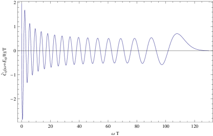
Figure 2: Fourier transform $\tilde{C}_{0}(\omega)$ of the uncoupled closed-channel amplitude, here evaluated for a Gaussian magnetic field pulse with the dimensionless energy $\varepsilon=100$. In the plot the numerically exact result is indistinguishable from the asymptotic evaluation as given by Eq. (63). As described in Section IV, $\tilde{C}_{0}(\omega)$ essentially determines the momentum distribution of the asymptotic dissociation state, see Eq. (IV.6). One observes that the spectrum does not exhibit a narrow peak-structure as one would require for atoms propagating with well-defined momenta. Rather, the spectrum exhibits contributions from all energies the pulse sweeps over. The oscillations stem from the interference between the contributions of the ascending and the descending slope of the pulse.

VI.3 Square-shaped magnetic field pulse

A clearer and more general insight into the relation between the pulse and the corresponding spectrum can be obtained by retreating to the stationary phase approximation. This comes at the cost of losing the spectrum in the tail region where the stationary points of the exponent in (62) leave the real axis. On the other hand, also non-analytic functions can now be treated. For the sake of simplicity, we consider symmetric pulses, $P(-\tilde{t})=P(\tilde{t})$. In stationary phase approximation, we then get from (62)

$$\frac{\tilde{C}_{0}(\omega+E_{0}/\hbar)}{T}=\sqrt{\frac{8\pi}{\varepsilon|P^{\prime}(\tilde{t}_{\omega})|}}\cos\left[\omega T\tilde{t}_{\omega}-\varepsilon\phi(\tilde{t}_{\omega})+\frac{\pi}{4}\right]\\ \text{for\ }\omega T/\varepsilon<\phi_{\max}^{\prime\prime},$$ (64)

where $\tilde{t}_{\omega}$ denotes the positive (dimensionless) stationary point, defined implicitly by $\phi^{\prime}(\tilde{t}_{\omega})=\omega T/\varepsilon$. Since $\tilde{t}_{\omega}$ is associated with the instant at which the pulse sweeps over the frequency $\omega$, it is manifest from (64) that the corresponding contribution to the spectrum is the more suppressed the faster the pulse sweeps over the corresponding energy, as one expects physically.

Aiming at a spectrum that is well-peaked at a specific energy, we thus must strive for magnetic field pulses that sweep as fast as possible over the region of undesired energies and then rest at a plateau determined by the desired energy. The (idealized) optimal pulse with that respect is a square-shaped pulse,

$$P(\tilde{t})=\Theta(\tilde{t}+1/2)\Theta(\tilde{t}-1/2),$$ (65)

for which (62) can be calculated directly, yielding

$$\frac{\tilde{C}_{0}(\omega+E_{0}/\hbar)}{T}= 2\pi\cos\left(\frac{\varepsilon}{2}\right)\delta(\omega T)$$

$$+\operatorname{sinc}\left(\frac{\omega T-\varepsilon}{2}\right)\mathcal{P}\left(\frac{\varepsilon}{\omega T}\right).$$ (66)

The pole at $\omega T=0$ can be traced back to the fact that the pulse function (65) is nonvanishing only on a finite time interval. For $E_{0}<0$, which corresponds to an asymptotic magnetic field in the bound regime, this pole lies at a negative energy irrelevant for the shape of the dissociation state, as was shown in Section IV. For our purposes it is thus sufficient to restrict the discussion to positive frequencies with $\omega+E_{0}/\hbar>0$. A plot of (VI.3) for $\varepsilon=100$ is shown in Figure 3. As anticipated, the spectrum exhibits a pronounced peak at $\omega T=\varepsilon$, whose width is characterized by the pulse duration $T$. According to (IV.6), the corresponding dissociation state therefore exhibits a narrow momentum distribution. This was used in Gneiting2009b where the two-particle momentum distribution generated by a square pulse has been worked out for a specific experimental scenario.

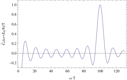
Figure 3: Fourier transform $\tilde{C}_{0}(\omega)$ of the uncoupled closed-channel amplitude component for a square-shaped magnetic field pulse with dimensionless energy $\varepsilon=100$. In contrast to the Gaussian pulse spectrum, it exhibits a pronounced peak at $\omega T=\varepsilon$. Together with the connection (IV.6) between $\tilde{C}(\omega)$ and the asymptotic dissociation state, this proves the capability of the scheme to provide relatively well-defined atom momenta, even though there is no way to tailor arbitrary dissociation states. In particular, sequences of such pulses then can serve to generate highly nonclassical motionally entangled states. (Since $E_{0}<0$ the pole at $\omega T=0$ does not affect the asymptotic behavior of the atoms.)

This concludes the quest for the optimal magnetic field pulse shape. As indicated in the stationary phase calculation (64), by sweeping as fast as possible over undesired energies one singles out a spectrum peaked at the desired energy. This has been verified numerically for a large variety of pulse forms. In particular, it is now clear that smoothening the edges of the square shape inevitably enhances the undesired ripples in the region of the energies swept over, contradicting the naive expectation that they stem from the non-differentiable ansatz (65) for the pulse.

More generally, we found that the nature of Feshbach dissociation dynamics puts strong limitations on the possible range of states that can be generated. It is in general not possible to find a pulse shape so as to generate a specified dissociation state. On the other hand, as was demonstrated in Gneiting2008a , the combination of a sequence of two dissociation pulses yields a promising perspective to generate highly nonclassical motionally entangled two-atom states with the capacity to violate a Bell inequality.

VII Conclusions

We described the dissociation of Feshbach molecules as triggered by a time-varying external magnetic field in a realistic trap and guide setting. Employing a coupled channels formulation including the center of mass motion, we derived an analytic expression for the asymptotic dissociation state in the laser guide. It is essentially determined by the Fourier transform of the closed-channel amplitude $C(t)$. The established relation between applied dissociation pulse and resulting spectrum $\tilde{C}(\omega)$ puts strong limitations on the possibility to tailor a pulse shape in order to obtain a desired dissociation state. However, a square-shaped magnetic field pulse is shown to optimize the momentum distribution with respect to its width, as it is required for subsequent interferometric processing.

The use of the Feshbach dissociation scheme as a source for entangled atom states was demonstrated in Gneiting2008a . There, a sequence of two equal magnetic field pulses dissociates the molecules such that each atom is delocalized into a pair of macroscopically separated, consecutive wave packets. Their subsequent interferometric processing on each side then constitutes a Bell test whose success requires a sharp momentum distribution as provided by the discussed square-shaped pulses.

An alternative protocol that can do without the interferometers employs a sequence of dissociation pulses of different heights. Given that the second pulse is the stronger one, the corresponding wave packets propagate faster as compared to the ones associated with the first pulse, such that time evolution alone effects their overlap. Position measurements in the overlap region on each side and their appropriate dichotomization may again reveal nonclassical correlations that entail a Bell violation.

One may also discard the restriction to the dissociation of a single pair and consider the simultaneous dissociation of a multitude of molecules in a multipair Bell setting Bancal2008a . Statistical effects due to the indistinguishability of the particles then require a theoretical treatment beyond the single-molecule dissociation dynamics. For this, the above derived two-body transition amplitude (between molecular initial state and asymptotic dissociation state) could serve as an essential building block, for example with respect to a cumulant expansion Kohler2002a .

References

- (1) I. Bloch, J. Dalibard, and W. Zwerger, Rev. Mod. Phys. 80, 885 (2008).
- (2) A. Buchleitner and A. R. Kolovsky, Phys. Rev. Lett. 91, 253002 (2003).
- (3) D. Witthaut, F. Trimborn, and S. Wimberger, Phys. Rev. Lett. 101, 200402 (2008).
- (4) M. Hartung, T. Wellens, C. A. Müller, K. Richter, and P. Schlagheck, Phys. Rev. Lett. 101, 020603 (2008).
- (5) J. Cubizolles, T. Bourdel, S. J. J. M. F. Kokkelmans, G. V. Shlyapnikov, and C. Salomon, Phys. Rev. Lett. 91, 240401 (2003).
- (6) S. Jochim et al., Phys. Rev. Lett. 91, 240402 (2003).
- (7) C. Regal, C. Ticknor, J. Bohn, and D. Jin, Nature 424, 47 (2003).
- (8) M. Greiner, C. Regal, and D. Jin, Nature 426, 537 (2003).
- (9) K. E. Strecker, G. B. Partridge, and R. G. Hulet, Phys. Rev. Lett. 91, 080406 (2003).
- (10) S. Dürr, T. Volz, A. Marte, and G. Rempe, Phys. Rev. Lett. 92, 020406 (2004).
- (11) J. Herbig et al., Science 301, 1510 (2003).
- (12) K. Xu et al., Phys. Rev. Lett. 91, 210402 (2003).
- (13) T. Kraemer et al., Nature 440, 315 (2006).
- (14) E. Donley, N. Claussen, S. Thompson, and C. Wieman, Nature 417, 529 (2002).
- (15) N. R. Claussen et al., Phys. Rev. A 67, 060701 (2003).
- (16) R. A. Duine and H. T. C. Stoof, Phys. Rep. 396, 115 (2004).
- (17) B. Borca, D. Blume, and C. H. Greene, New J. Phys. 5, 111 (2003).
- (18) K. Góral, T. Köhler, and K. Burnett, Phys. Rev. A 71, 023603 (2005).
- (19) K. V. Kheruntsyan, M. K. Olsen, and P. D. Drummond, Phys. Rev. Lett. 95, 150405 (2005).
- (20) K. V. Kheruntsyan, Phys. Rev. Lett. 96, 110401 (2006).
- (21) S. Dürr et al., Phys. Rev. A 72, 052707 (2005).
- (22) T. M. Hanna, K. Góral, E. Witkowska, and T. Köhler, Phys. Rev. A 74, 023618 (2006).
- (23) T. Mukaiyama, J. Abo-Shaeer, K. Xu, J. Chin, and W. Ketterle, Phys. Rev. Lett. 92, 180402 (2004).
- (24) S. Dürr, T. Volz, and G. Rempe, Phys. Rev. A 70, 031601 (2004).
- (25) C. Gneiting and K. Hornberger, Phys. Rev. Lett. 101, 260503 (2008).
- (26) C. Gneiting and K. Hornberger, Appl. Phys. B 95, 237 (2009).
- (27) J. Brendel, N. Gisin, W. Tittel, and H. Zbinden, Phys. Rev. Lett. 82, 2594 (1999).
- (28) W. Tittel, J. Brendel, H. Zbinden, and N. Gisin, Phys. Rev. Lett. 84, 4737 (2000).
- (29) T. Köhler, K. Góral, and P. Julienne, Rev. Mod. Phys. 78, 1311 (2006).
- (30) N. Nygaard, R. Piil, and K. Mølmer, Phys. Rev. A 78, 023617 (2008).
- (31) F. H. Mies, E. Tiesinga, and P. S. Julienne, Phys. Rev. A 61, 022721 (2000).
- (32) C. Gneiting and K. Hornberger, Opt. Spectrosc. 108, 188 (2010); eprint arXiv:0905.1279.
- (33) S. Jochim et al., Science 302, 2101 (2003).
- (34) J. R. Taylor, Scattering Theory: The Quantum Theory on Nonrelativistic Collisions (Wiley, New York, 1972).
- (35) M. Olshanii, Phys. Rev. Lett. 81, 938 (1998).
- (36) N. Bleistein and R. A. Handelsman, Asymptotic Expansions of Integrals (Dover, New York, 1986).
- (37) J.-D. Bancal et al., Phys. Rev. A 78, 062110 (2008).
- (38) T. Köhler and K. Burnett, Phys. Rev. A 65, 033601 (2002).