Abstract

Fractional generalizations of the Poisson process and branching Furry process are considered. The link between characteristics of the processes, fractional differential equations and Lèvy stable densities are discussed and used for construction of the Monte Carlo algorithm for simulation of random waiting times in fractional processes. Numerical calculations are performed and limit distributions of the normalized variable $Z=N/\langle N\rangle$ are found for both processes.

Keywords: fractional Poisson process, fractional Furry process, one-sided stable density

1 Introduction

The Poisson process is the simplest but the most important model for physical and other applications. Its main properties (absence of memory and jump-shaped increments) model a large number of natural and social processes. Basic equations of theoretical physics (Schroedinger’s, Pauly’s, Dirac’s and other equations) are derived in frame of axioms of the Poisson process. These equations describe fundamental processes on a microscopic physical level.

When investigating complex macroscopic systems, we can observe another kind of behavior showing the presence of memory.

There exist a few fractional generalizations of the Poisson process [Repin & Saichev, 2000, Jumarie Guy, 2001, Wang Xiao-Tian & Wen Zhi-Xiong, 2003, Wang Xiao-Tian et al., 2006, Laskin, 2003]. We consider here the fractional Poisson process (fPp), introduced by the waiting time distribution density $\psi_{\nu}(t)$ with the Laplace transform

$$\widetilde{\psi}_{\nu}(\lambda)\equiv\int\limits_{0}^{\infty}e^{-\lambda t}\psi_{\nu}(t)dt=\frac{\mu}{\mu+\lambda^{\nu}}.$$ (1)

The density is characterized by fractional exponent $\nu\in(0,1]$, being the order of the fractional differential equation describing this process. When $\nu=1$, the fPp becomes the standard Poisson process,

$$\widetilde{\psi}_{1}(\lambda)=\frac{\mu}{\mu+\lambda},\quad\psi_{1}(t)=\mu e^{-\mu t};$$

when $\nu<1$, the fPp displays the property of memory, namely, the correlations between events in non-overlapping time intervals arise. Thus, the memory is a function of the parameter $\nu$ that makes the fPp very attractive for investigating the mathematical phenomenology of memory.

We consider in this work the main properties of the fPp, reformulate them in terms of alpha-stable densities , construct an algorithm for simulation of interarrival time, apply it to Monte Carlo simulation of the fPp, and find limit distributions. On the base of this approach we will introduce also the fractional generalization of the simplest branching process and find the correspondent distributions. But first of all we’ll bring some physical reasons of our interest to the fPp.

2 Physics of fPp

For the sake of clearness, let us talk about number of events $N(t)$ as about coordinate of a particle performing spasmodic motion in a given direction. The particle, appeared at the origin at time $t=0$, stays there some random time $T_{1}$, then makes a jump to the position $N=1$, stays there random time $T_{2}$, then the second jump to $N=2$ and so forth. Suppose that all $T_{j}$ are independent and identically distributed random variables. Let $Q(t)=\textsf{P}(T>t)$. If $Q(t)=e^{-\mu t},\ \mu>0$, then $N(t)$ is the Poisson process with rate $\mu$. If the distribution of $T$ is not an exponential one, but $\langle T\rangle<\infty$, the process is not a Poisson one, but at large scales it looks like a Poisson process and could be called the asymptotically Poisson process. As in the first case, the motion of the particle considered at large scales will seem to be almost regular and uniform with the "velocity" $1/\langle T\rangle$. There are no special asymptotical properties which appear here.

The situation changes when $Q(t)$ has a power law long tail

$$Q(t)\propto t^{-\nu},\ 0<\nu<1,$$ (2)

and an infinite mathematical expectation $\langle T\rangle$. Namely this type of traps leads to a fractional generalization of the Poisson process.

The physical grounds of (2) has been discussed in a number of works. The first of interpretation of (2) has been done by Tunaley [1972] on the base of the following simple jump mechanism. The process goes in an insulator containing randomly distributed point (of small size) traps with exponentially distributed waiting times: $\textsf{P}\{T>t|\theta\}=\exp(-t/\theta)$. Their mean value $\theta$ is finite and linked with the random distant $\delta$ to the nearest site in the direction of the applied field as follows [Harper, 1967]:

$$\theta=\beta[\exp(\gamma\delta)-1].$$

Here, $\gamma$ is a positive constant and $\beta$ is inversely proportional to the applied potential gradient, both are independent of the temperature of the sample. Taking for $\delta$ the exponential distribution with the mean $d$,

$$\textsf{P}\{\delta>x\}=e^{-x/d},$$

we obtain the probability density for $\theta$ in the following form

$$\textsf{P}\{\theta>t\}=\textsf{P}\{\delta>(1/\gamma)\ln(1+t/\beta)\}=\exp[-(1/\gamma d)\ln(1+t/\beta)]=(1+t/\beta)^{-1/(\gamma d)}.$$

Averaging these distribution over $d$

$$\textsf{P}\{T>t\}=-\int\limits_{0}^{\infty}\textsf{P}\{T>t|t^{\prime}\}d\textsf{P}\{\theta>t^{\prime}\}\sim\nu\Gamma(\nu)(t/\beta)^{-\nu},\ t\rightarrow\infty,\ \nu=1/(\gamma d)$$

yields (2).

In [Scher & Montroll, 1975], it has been indicated that the dispersive behavior can be caused also by multiple trapping in a distribution of localized states. On the assumption that the localized states below the mobility edge fall off exponentially with energy, one can arrive at Eq. (2) with the exponent $\nu$ depending on the temperature $\Theta=kT$. In the frame of this model, called random activated energy model it is assumed, that

(i) the jump rate of a particle hopping over an energy barrier $\Delta E$ has the usual quasiclassical form

$$W=Ae^{-\Delta E/\Theta};$$

(ii) the conditional waiting time distribution corresponding to a given activation energy $\Delta E=\varepsilon$ is exponential

$$\textsf{P}\{T>t|\varepsilon\}=e^{-W(\varepsilon)t};$$

and

(iii) the activation energy is a random variable with the Boltzman distribution density

$$p(\varepsilon)=(\Theta_{\rm c})^{-1}e^{-\varepsilon/\Theta_{\rm c}}.$$

Averaging over the activation energy results:

$$\textsf{P}\{T>t\}=\int\limits_{0}^{\infty}\textsf{P}\{T>t|\varepsilon\}p(\varepsilon)d\varepsilon=\int\limits_{0}^{\infty}\exp[-(Ae^{-\varepsilon/\Theta})t]\ d(e^{-\varepsilon/\Theta_{\rm c}})=\nu\Gamma(\nu)(At)^{-\nu}$$

with $\nu=\Theta/\Theta_{\rm c}$. Here, $\Theta_{\rm c}$ is the characteristic temperature defining the conduction band tail. For $\Theta<\Theta_{\rm c}$, thermalization dominates and the photoinjected carriers sink progressively deeper in increasing time; the transport becomes dispersive. For $\Theta>\Theta_{\rm c}$, the carriers remain concentrated near the mobility edge and the charge transit exhibit non-dispersive behavior. Consequently, the physical meaning of $\nu$ is that it is representative of disorder: the smaller its value the more dispersive the transport.

The fluorescence emission of single semiconductor colloidal nanocrystals such as CdSe/ZnS core-shell quantum dots (QDs), exhibits unusual intermittency behavior [Shimizu et al. 2001]. Under laser illumination, nanocrystals blink: QDs jumps between bright and dark states. Experimental investigations of blinking QD fluorescence showed that on- and off-periods are distributed according to inverse power laws with exponents and respectively. The mechanism of QD’s blinking is not yet quite understood. Thermally activated ionization, electron tunnelling through fluctuating barriers and some other mechanisms were suggested as alternative ones yielding power on- and off-time distributions. An emission wavelength of QD fluorescence is simply tuned by changing the size of the nanocrystal. This makes them promising as the active medium in light-emitting diodes or lasers. Fluctuations in the intensity of QD fluorescence can limit such applications. From theoretical results one follows that fluctuations in the case of power on- and off-intervals distributions stay constant and not decrease with time.

These theoretical results being in accordance with numerous experimental data represent additional physical reasons for high attention to the fractional Poisson process, fractional differential equations and long memory phenomena models.

3 Waiting time density

The fPp waiting time density $\psi_{\nu}(t)$ can be represented in three equivalent forms. The first of them, given in [Repin & Saichev, 2000], is

$$\psi_{\nu}(t)=\frac{1}{t}\int\limits_{0}^{\infty}e^{-x}\phi_{\nu}(\mu t/x)dx,$$

where

$$\phi_{\nu}(\xi)=\frac{\sin(\nu\pi)}{\pi[\xi^{\nu}+\xi^{-\nu}+2\cos(\nu\pi)]}.$$

This form allows to find asymptotical expressions for small and large time,

$$\psi(t)\sim{\frac{\mu^{\nu}}{\Gamma(\nu)}t^{\nu-1}},\quad t\to 0,$$

$$\psi(t)\sim\frac{\nu\mu^{-\nu}}{\Gamma(1-\nu)}t^{-\nu-1},\quad t\to\infty,$$

and to perform numerical calculations of the density (see Fig 1.).

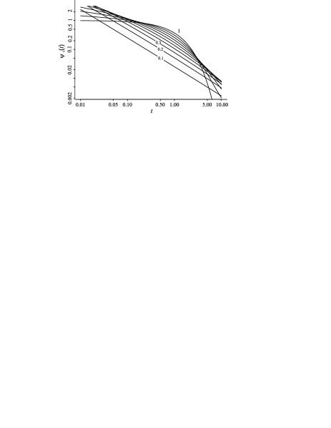
Figure 1: The fPp waiting time distribution densities (3) for $\mu=1$ and $\nu=0.1(0.1)1.$

The second form, obtained in [Laskin 2003],

$$\textsf{P}(T>t)=E_{\nu}(-\mu t^{\nu}),$$

$$\psi_{\nu}(t)=-\frac{d\textsf{P}(T>t)}{dt}=\mu t^{\nu-1}E_{\nu,\,\nu}(-\mu t^{\nu})$$ (3)

uses the Mittag-Leffler functions

$$E_{\alpha}(z)=\sum\limits_{n=0}^{\infty}\frac{z^{n}}{\Gamma(\nu n+1)},$$

$$E_{\alpha,\,\beta}(z)=\sum_{n=0}^{\infty}\frac{z^{n}}{\Gamma(\alpha n+\beta)}.$$

We present here the third form, which will serve as a basis for Monte Carlo simulation of fPp’s.

The complement cumulative distribution function $\textsf{P}(T>t)$ can be represented in the form

$$\textsf{P}(T>t)=\int\limits_{0}^{\infty}e^{-\mu t^{\nu}/\tau^{\nu}}g^{(\nu)}(\tau)d\tau,$$ (4)

where $g^{(\nu)}(\tau)$ is the one-sided $\alpha$-stable density (see for details [Uchaikin & Zolotarev 1999], [Uchaikin 2003], [Dubkov & Spagnolo 2005] and [Dubkov & Spagnolo 2007]).

Indeed, expanding the exponential function in (4)

$$e^{-\mu t^{\nu}/\tau^{\nu}}=\sum_{k=0}^{\infty}\frac{1}{k!}(-\mu t^{\nu}/\tau^{\nu})^{k}$$

and making use of the formula for negative order moments of the $\alpha$-stable-density

$$\int\limits_{0}^{\infty}g^{(\nu)}(\tau)\tau^{-\nu k}d\tau=\frac{k!}{\Gamma(1+\nu k)},$$

we obtain

$$\textsf{P}(T>t)=\sum_{k=0}^{\infty}\frac{(-\mu t^{\nu})^{k}}{k!}\int\limits_{0}^{\infty}\tau^{-\nu k}g^{(\nu)}(\tau)d\tau=\sum_{k=0}^{\infty}\frac{(-\mu t^{\nu})^{k}}{\Gamma(1+\nu k)}=E_{\nu}(-\mu t^{\nu}).$$

4 Simulation of waiting times

The following result solves the problem of simulation of random waiting times.

The random variable $T$ determined above has the same distribution as

$$T^{\prime}=\frac{|\ln U|^{1/\nu}}{\mu^{1/\nu}}S(\nu),$$

where $S(\nu)$ is a random variable distributed according to $g^{(\nu)}(\tau)$ and $U$ is independent of $S(\nu)$, is a uniformly distributed in $[0,1]$ random variable.

Making use of the formula of total probability, let us represent (4) in the following form

$$\textsf{P}(T>t)=\int\limits_{0}^{\infty}\textsf{P}(T>t|\tau)g^{(\nu)}(\tau)d\tau,$$

where

$$\textsf{P}(T>t|\tau)=e^{-\mu t^{\nu}/\tau^{\nu}}$$

is the conditional distribution. This means that

$$\textsf{P}(T>t|\tau)=\textsf{P}(U<e^{-\mu t^{\nu}/\tau^{\nu}})=\textsf{P}\left(\frac{|\ln U|^{1/\nu}}{\mu^{1/\nu}}\tau>t\right),$$

or

$$T|_{\tau}\stackrel{{\scriptstyle d}}{{=}}\frac{|\ln U|^{1/\nu}}{\mu^{1/\nu}}\tau.$$

Because $\tau$ is a fixed possible value of $S(\nu)$, we obtain for unconditional interarrival time

$$T\stackrel{{\scriptstyle d}}{{=}}\frac{|\ln U|^{1/\nu}}{\mu^{1/\nu}}S(\nu).$$

The random variable

$$T\stackrel{{\scriptstyle d}}{{=}}\frac{|\ln U_{1}|^{1/\nu}}{\mu^{1/\nu}}\frac{\sin(\nu\pi U_{2})[\sin((1-\nu)\pi U_{2})]^{1/\nu-1}}{[\sin(\pi U_{2})]^{1/\nu}[\ln U_{3}]^{1/\nu-1}},$$ (5)

where $U_{1},\ U_{2}$ and $U_{3}$ are independent uniformly distributed on [0,1] random numbers. This conclusion follows from the Kanter algorithm for simulating $S(\nu)$ [Kanter, 1975].

Note that when $\nu\to 1$ this algorithm reduces to standard rule of simulating random numbers with exponential distribution:

$$T\stackrel{{\scriptstyle d}}{{=}}\frac{|\ln U|}{\mu}.$$

5 The $n$th arrival time distribution

Let $T^{(n)},\ n=1,2,3,\dots,$ be the $n$th arrival time of fPp

$$T_{n}=T^{(1)}+T^{(2)}+\cdots+T^{(n)}$$

and $\psi^{*n}(t)$ be its probability density :

$$\psi^{*n}(t)= \underbrace{\psi*\psi*\cdots*\psi}(t).$$

$$n$$ times

Here, $T^{(j)}$’s are mutually independent copies of the interarrival random times $T$ and symbol $*$ denotes the convolution operation

$$\psi*\psi(t)\equiv\int\limits_{0}^{t}\psi(t-\tau)\psi(\tau)d\tau.$$

For the standard Poisson process,

$$\psi^{*n}(t)=\mu\frac{(\mu t)^{n-1}}{(n-1)!}e^{-\mu t},$$

and according to the Central Limit Theorem

$$\Psi^{(n)}(t)\equiv(\sqrt{n}/\mu)\psi^{*n}(n/\mu+t\sqrt{n}/\mu)\Rightarrow\frac{1}{\sqrt{2\pi}}e^{-t^{2}/2},\ n\to\infty.$$

As numerical calculations show, $\Psi^{(n)}(t)$ practically reaches its limit form already by $n=10$ (Fig. 2).

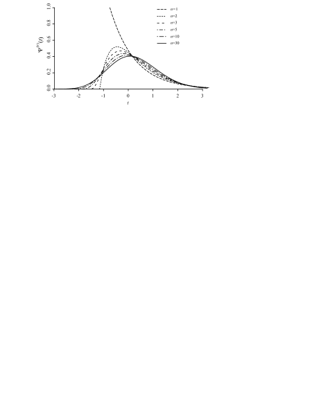
Figure 2: Rescaled arrival time distributions for the standard Poisson process $({\nu=1,n=1,2,3,5,10,30})$.

In case of the fPp,

$$\textsf{E}T=\int\limits_{0}^{\infty}\psi_{\nu}(t)tdt=\infty$$

and the Central limit theorem is not applicable. Applying the Generalized limit theorem (see, for example, [Uchaikin & Zolotarev, 1999]), we obtain:

$$\Psi_{\nu}^{(n)}(t)\equiv\left(\frac{n}{\mu}\right)^{1/\nu}\psi_{\nu}^{*n}\left(t\left(\frac{n}{\mu}\right)^{1/\nu}\right)=n^{1/\nu}\stackrel{{\scriptstyle\circ}}{{\psi}}_{\nu}^{*n}(tn^{1/\nu})\Rightarrow g^{(\nu)}(t),\ n\to\infty,$$

where

$$\stackrel{{\scriptstyle\circ}}{{\psi}}_{\nu}(t)=\psi_{\nu}(t)|_{\mu=1}=t^{\nu-1}E_{\nu,\,\nu}(-t^{\nu}).$$

Computing this multiple integrals can be performed by Monte Carlo technique. Taking $\mu=1$ and observing that $\Psi_{\nu}^{n}(t)$ is the probability density of the renormalized sum $(T_{1}+T_{2}+\dots+T_{n})/n^{1/\nu}$ of independent random variable, distributed according to $\stackrel{{\scriptstyle\circ}}{{\psi}}_{\nu}(t)$, we could directly simulate this sum by making use of the algorithm given by Eq. (5) and construct the corresponding histogram. However, the left tail of the densities is too steep for this method, and we applied some modification of Monte Carlo method based on the partial analytical averaging of the last term.

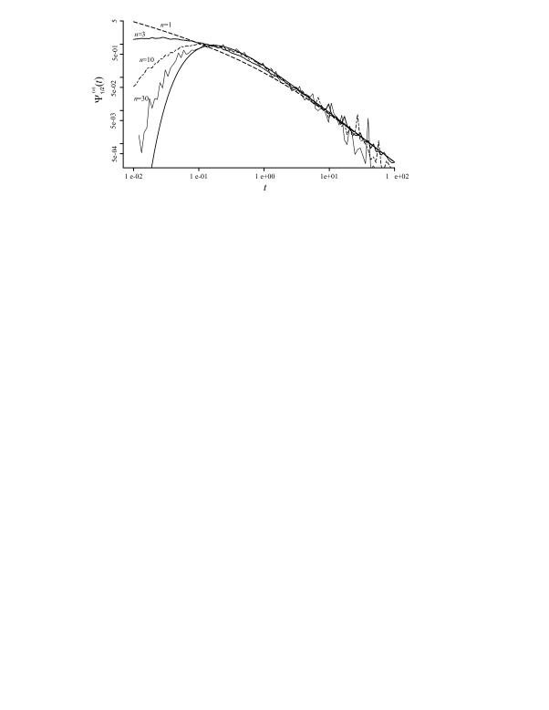
Figure 3: Rescaled arrival time distributions for fPp ($\nu=1/2;n=1,3,10,$ and 30).

By making use of this modification, we computed the distributions $\Psi_{\nu}^{(n)}(t)$ for various $n$ and $\nu$. An example of these results is represented in Fig. 3.

6 The fractional Poisson distribution

Now we consider another random variable: the number of events (pulses) $N(t)$ arriving during the period $t$. According to the theory of renewal processes

$$p_{n}(t)\equiv\textsf{P}(N(t)=n)=\textsf{P}\left(\sum\limits_{j=1}^{n}T_{j}>t\right)-\textsf{P}\left(\sum\limits_{j=1}^{n+1}T_{j}>t\right),\quad n=0,1,2,\dots$$

and the following system of integral equations for $p_{n}(t)$ takes place:

$$p_{n}(t)=\delta_{n0}\int\limits_{t}^{\infty}\psi_{\nu}(\tau)d\tau+[1-\delta_{n0}]\int\limits_{0}^{t}\psi_{\nu}(t-\tau)p_{n-1}(\tau)d\tau,\quad n=0,1,2,\dots$$

After the Laplace transform with respect to time, we obtain

$$\lambda^{\nu}\widetilde{p}_{n}(\lambda)=-\mu\widetilde{p}_{n}(\lambda)+\mu\widetilde{p}_{n-1}(\lambda)+\lambda^{\nu-1}\delta_{n0},$$

$$n=0,1,2,\dots,\qquad\widetilde{p}_{-1}=0.$$

The inverse Laplace transform yields:

$$_{0}D_{t}^{\nu}p_{n}(t)=\mu[p_{n-1}(t)-p_{n}(t)]+\frac{t^{-\nu}}{\Gamma(1-\nu)}\delta_{n0},\ 0<\nu\leq 1.$$ (6)

This is a master equation system for the fractional Poisson processes. When $\nu\to 1$ it becomes the well known system for the standard Poisson process:

$$\frac{dp_{n}(t)}{dt}=\mu[p_{n-1}(t)-p_{n}(t)]+\delta(t)\delta_{n0}.$$ (7)

System (6) produces for the generating function

$$g(u,t)\equiv\sum\limits_{n=0}^{\infty}u^{n}p_{n}(t)$$ (8)

the following equation:

$$_{0}D_{t}^{\nu}g(u,t)=\mu(u-1)g(u,t)+\frac{t^{-\nu}}{\Gamma(1-\nu)}.$$ (9)

When $\nu\to 1$ it becomes the well known equation for the standard Poisson process:

$$\frac{dg(u,t)}{dt}=\mu(u-1)g(u,t)+\delta(t).$$ (10)

Comparing (6) with (7) and (9) with (10), one can observe that the equations for standard processes are generalized to the equations for correspondent fractional processes by means of replacement of the operator $d/dt$ with ${}_{0}D_{t}^{\nu}$ and of right side the term $\delta(t)$ with $t^{-\nu}/\Gamma(1-\nu)$.

The solution to Eq. (9) is of the form

$$g(u,t)=E_{\nu}(\mu(u-1)t^{\nu})\equiv\sum\limits_{n=0}^{\infty}\frac{a^{n}}{\Gamma(\nu n+1)}(u-1)^{n},\ a=\mu t^{\nu}.$$

Applying the binomial formula to each term of the sum and interchanging the summations, one can rewrite it as the series

$$g(u,t)=\sum\limits_{n=0}^{\infty}u^{n}\left[\frac{a^{n}}{n!}\sum\limits_{m=0}^{\infty}\frac{(m+n)!(-a)^{m}}{m!\Gamma(\nu(mk+n)+1)}\right].$$ (11)

Comparing (11) with (8) yields

$$p_{n}(t)=\frac{a^{n}}{n!}\sum\limits_{m=0}^{\infty}\frac{(m+n)!}{m!}\frac{(-a)^{m}}{\Gamma((m+n)\nu+1)}.$$

This distribution, which becomes the Poisson one when $\nu=1$ can be considered as its fractional generalization, called fractional Poisson distribution. The correspondent mean value and variance are given by

$$\langle N(t)\rangle=\frac{\mu t^{\nu}}{\Gamma(\nu+1)}$$

and

$$\sigma^{2}(t)=\langle N(t)\rangle\{1+\langle N(t)\rangle[2^{1-2\nu}\nu\mathrm{B}(\nu,1/2)-1]\},$$

where

$$\mathrm{B}(\alpha_{1},\alpha_{2})=\int\limits_{0}^{1}x^{\alpha_{1}-1}(1-x)^{\alpha_{2}-1}dx$$

is the beta-function.

7 Limit fractional Poisson distributions

In case of the standard Poisson process, the probability distribution for random number $N(t)$ of events follows the Poisson law with $\langle N(t)\rangle=\mu t=\overline{n}$ which approaches to the normal one at large $\overline{n}$. Introducing normalized random variable $Z=N(t)/\overline{n}$ and quasicontinuous variable $z=n/\overline{n}$, one can express the last fact as follows:

$$f(z;\overline{n})=\overline{n}\frac{\overline{n}^{\overline{n}z}}{\Gamma(\overline{n}z+1)}e^{-\overline{n}}\sim$$

$$\sim\sqrt{\frac{\overline{n}}{2\pi}}\exp\left\{-\frac{(z-1)^{2}}{2/\overline{n}}\right\}$$

as $\quad\overline{n}\to\infty$. In the limit case $\overline{n}\to\infty$ the distribution of $Z$ becomes degenerated one:

$$\lim\limits_{\overline{n}\to\infty}f(z;\overline{n})=\delta(z-1).$$

Considering the case of fPp, we pass from the generating function to the Laplace characteristic function

$$g(u,t)=E_{\nu}(\mu t^{\nu}(u-1))=E_{\nu}(\overline{n}\Gamma(\nu+1)(u-1)).$$

Introducing a new parameter $\lambda=-\overline{n}\ln u$ we get

$$\textsf{E}u^{N(t)}=\textsf{E}e^{-\lambda Z}=E_{\nu}(\overline{n}\Gamma(\nu+1)(e^{-\lambda/\overline{n}}-1)).$$

At large $\overline{n}$ relating to large time $t$,

$$\textsf{E}e^{-\lambda Z}\equiv\int\limits_{0}^{\infty}e^{-\lambda z}f_{\nu}(z)dz\sim E_{\nu}(-\lambda^{\prime}),$$

$$\lambda^{\prime}=\lambda\Gamma(\nu+1).$$

Comparison of this equation with formula (6.9.8) of the book [Uchaikin & Zolotarev, 1999]

$$E_{\nu}(-\lambda^{\prime})=\nu^{-1}\int\limits_{0}^{\infty}\frac{e^{-\lambda^{\prime}x}}{x^{1+1/\nu}}g^{(\nu)}(x^{-1/\nu})dx=\int\limits_{0}^{\infty}e^{-\lambda z}\ \frac{[\Gamma(\nu+1)]^{1/\nu}}{\nu\ z^{1+1/\nu}}g^{(\nu)}\left(\frac{z^{-1/\nu}}{[\Gamma(\nu+1)]^{-1/\nu}}\right)dz$$

shows that the random variable $Z$ has the non-degenerated limit distribution at $t\to\infty$ (see also [Uchaikin, 1999]):

$$f_{\nu}(z;\overline{n})\to f_{\nu}(z)=\frac{[\Gamma(\nu+1)]^{1/\nu}}{\nu\ z^{1+1/\nu}}g^{(\nu)}\left(\frac{z^{-1/\nu}}{[\Gamma(\nu+1)]^{-1/\nu}}\right)$$ (12)

with moments

$$\langle Z^{k}\rangle=\frac{[\Gamma(1+\nu)]^{k}\Gamma(1+k)}{\Gamma(1+k\nu)}.$$

By making use of series for $g^{(\nu)}$, we obtain

$$f_{\nu}(z)=\sum_{k=0}^{\infty}\frac{(-z)^{k}}{k!\Gamma(1-(k+1)\nu)[\Gamma(\nu+1)]^{k+1}}.$$

When $z\to 0$,

$$f_{\nu}(z)\to f_{\nu}(0)=\frac{1}{\Gamma(1+\nu)\Gamma(1-\nu)}=\frac{\sin(\nu\pi)}{\nu\pi}.$$

It is also worth to note, that $\langle Z^{0}\rangle=1,\ \langle Z^{1}\rangle=1$ and $\langle Z^{2}\rangle=2\nu{\rm B}(\nu,1+\nu)$, so that the limit relative fluctuations are given by

$$\delta_{\nu}\equiv\sigma_{N(t)}/\langle N\rangle=\sqrt{2\nu{\rm B}(\nu,1+\nu)-1}.$$

In particular cases

$$\delta_{0}=1,\quad\delta_{1}=0,\quad\delta_{1/2}=\sqrt{\pi/2}-1.$$

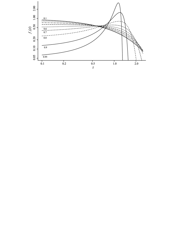
Figure 4: Limit distributions (12) for $\nu=0.1(0.1)0.9$ and 0.95.

For $\nu=1/2$, one can obtain an explicit expression for $f_{\nu}(z)$ :

$$f_{1/2}(z)=\frac{2}{\pi}e^{-z^{2}/\pi},\ z\geq 0.$$

The family of this limit distributions are plotted in Fig. 4.

8 Fractional Furry process

Let us pass to the branching processes and consider its simplest case, when each particle converts into two identical ones at the end of its waiting time, distributed with density $\psi_{\nu}(t)$. The process begins with one particle at $t=0$ and the first arrival time has the same distribution density $\psi_{\nu}(t)$. When $\nu=1$, the process is called the Furry process (Fp), therefore, in case of $\nu<1$ we can call it the fractional Furry process (fFp). The following integral equations govern the fFp:

$$p_{n}(t)=\delta_{n1}\int\limits_{t}^{\infty}\psi_{\nu}(\tau)d\tau+[1-\delta_{n0}-\delta_{n1}]\int\limits_{0}^{t}\psi_{\nu}(t-\tau)\sum\limits_{k=1}^{n-1}p_{k}(\tau)p_{n-k}(\tau)d\tau,\quad n=1,2,\dots$$

Following the same way as before, we obtain

$${}_{0}D_{t}^{\nu}p_{n}(t)=\mu\left[\sum\limits_{k=1}^{n-1}p_{k}(t)p_{n-k}(t)-p_{n}(t)\right]+\frac{t^{-\nu}}{\Gamma(1-\nu)}\delta_{n1},\ 0<\nu\leq 1.$$

The solution of this equation in case of $\nu=1$ is well known: it is represented by the geometrical distribution

$$p_{n}(t)=e^{-\mu t}\left[1-e^{-\mu t}\right]^{n-1},\ n=1,2,3,\dots$$

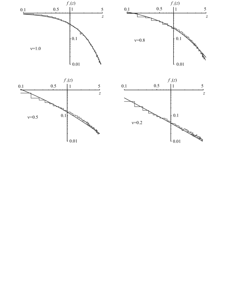
Figure 5: Monte Carlo calculation of $f_{\nu}(z)$ for $t=5$ and $\nu=1.0,\ 0.8,\ 0.5,\ 0.2$ (histograms) by comparison with hypothetical distribution (13) (smooth lines).

As to fFp for $\nu<1$, we did not manage to derive the corresponding distribution from the fractional equation in a closed analytical form. The reason of the trouble lies in nonlinearity of the equation in case of branching. The only characteristics, the mean number of particles at time $t$ has been found and expressed through the Mittag-Leffler function:

$$\langle N(t)\rangle=E_{\nu}(\mu t^{\nu}).$$

All other results have been obtained by means of Monte Carlo simulation using the algorithm described above.

Observe, that in contrast to the fPp, the limit distribution of the normalized random variable $Z$ in case of fFp is not degenerated. In particular, for the standard Furry process

$$f(z)=\lim\limits_{\overline{n}\to\infty}\overline{n}p_{\overline{n}z}(\mu^{-1}\ln\overline{n})=e^{-z}.$$

One could to suppose that in fractional case the "standard exponential function" is replaced with its fractional analogue

$$f_{\nu}(z)=z^{\nu-1}E_{\nu,\nu}(-z^{\nu}).$$ (13)

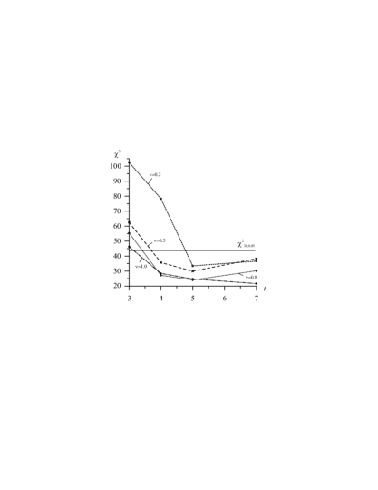
Figure 6: $\chi^{2}$ Goodness-of fit Test.

Direct comparison of Monte Carlo data with formula (13) (Fig. 5) allows to propose that they coincide at large $t$, and the $\chi^{2}$ goodness of fit analysis confirms this hypothesis (Fig. 6).

9 Concluding remarks

Considering the fractional Poisson process as an example of integer-valued fractional processes, one can suppose that the use of $\alpha$-stable densities may occur very useful both for theoretical investigations and numerical simulations. Another example of integer-valued fractional processes, Furry branching process, has been too considered. We are planning to continue this work by analyzing binomial, negative binomial and some other integer-valued processes which can be useful for description of stochastic phenomena in laser physics, quantum optics and even in quantum chromodynamics i.e. quark-gluon plasma statistics [Botet & Ploszajczak, 2002].

This work is supported by Russian Foundation for Basic Research (project 07-01-00517).

References

- [1] Botet, R. & Ploszajczak, M. [2002] Universal Fluctuations: The Phenomenology of Hadronic Matter (World Scientific Publishing Co. Pte. Ltd, New Jersey) 369 p.
- [2] Dubkov, A. A. & Spagnolo, B. [2005] ‘‘Generalized Wiener Process and Kolmogorov’s Equation for Diffusion Induced by Non-Gaussian Noise Source,’’ Fluctuation and Noise Letters 5 (2), L267-L274.
- [3] Dubkov, A. A. & Spagnolo, B. [2007] ‘‘Langevin Approach to Anomalous Diffusion in fixed potentials: exact results for stationary probability distributions,’’ Acta Physica Polonica B 38 (5), 1745-1758.
- [4] Harper, W. R. [1967] Contact and Frictional Electrification (Oxford Univ. Press, Oxford).
- [5] Jumarie Guy [2001] ‘‘Fractional master equation: non-standard analysis and Liouville-Riemann derivative,’’ Chaos, Solitons and Fractals 12, 2577-2587.
- [6] Kanter, M. [1975] ‘‘Stable densities under change of scale and total variation inequalities,’’ Ann. Probab. 3, 697-707.
- [7] Laskin, N. [2003] ‘‘Fractional Poisson Process,’’ Communications in Nonlinear Science and Numerical Simulation 8, 201-213.
- [8] Repin, O. N. & Saichev, A. I. [2000] ‘‘Fractional Poisson Law,’’ Radiophysics and Quantum Electronics 43(9), 738-741.
- [9] Scher, H. & Montroll, E. W. [1975] ‘‘Anomalous transit-time dispersion in amorphous solids,’’ Physical Review B 12, 2455-2477.
- [10] Shimizu, K. T. et al. [2001] ‘‘Blinking statistics in single semiconductor nanocrystal quantum dots,’’ Phys. Rev. B 63 205316-1-205316-5.
- [11] Tunaley, J. K. E. [1972] ‘‘A physical process for noise in thin metallic films,’’ J. Appl. Phys. 43, 3851-3855. ‘‘Some stochastic processes yielding a type of spectral density,’’ J. Appl. Phys. 43, 4777-4783. ‘‘Conduction in a random lattice under a potential gradient,’’ J. Appl. Phys. 43, 4783-4786.
- [12] Uchaikin, V. V. & Zolotarev, V. M. [1999] Chance and Stability: Stable Distributions and their Applications (VSP, Ultrecht, The Netherlands) 570 p.
- [13] Uchaikin, V. V. [1999] ‘‘Subdiffusion and stable laws,’’ Journal of Experimental and Theoretical Physics 88(6), 1155-1163.
- [14] Uchaikin, V. V. [2003] ‘‘Self-similar anomalous diffusion and Levy-stable laws’’, Physics-Uspekhi 46(8), 821-849.
- [15] Wang Xiao-Tian & Wen Zhi-Xiong [2003] ‘‘Poisson fractional processes,’’ Chaos, Solitons and Fractals 18, 169-177.
- [16] Wang Xiao-Tian, Wen Zhi-Xiong & Zhang Shi-Ying [2006] ‘‘Fractional Poisson process’’ Chaos, Solitons and Fractals 28, 143-147.