Quantum Spin Tomography in Ferromagnet-Normal Conductors

Abstract

We present a theory for a complete reconstruction of non-local spin correlations in ferromagnet-normal conductors. This quantum spin tomography is based on cross correlation measurements of electric currents into ferromagnetic terminals with controllable magnetization directions. For normal injectors, non-local spin correlations are universal and strong. The correlations are suppressed by spin-flip scattering and, for ferromagnetic injectors, by increasing injector polarization.

Spintronics utilizes the electron spin in electronics applications and is an important subfield of condensed matter physics. It is possible to create metallic or semiconducting hybrid ferromagnet-normal conductor systems smaller than the spin-flip length mesospin ; spindot , yet semiclassically large. Topics of current interest such as spin injection, precession, and relaxation mesospin ; spindot ; Johnsil , spin Hall effects Spinhall , current induced magnetization excitations RalphStiles , the reciprocal magnetization dynamics induced spin-pumping Arnerev , spin based transistors Dattadas , and ferromagnet-superconductor heterostructures FS focus on the average non-equilibrium spin accumulation and dynamics.

The correlations between injected spins in ferromagnet-normal conductor systems have received much less attention. In two-terminal junctions, current correlations have been investigated in few-level quantum dots Bulka as well as semiclassically large systems Twoterm ; Arne . The prime targets have been noise due to spin-flip scattering and the super or sub poissionian nature of the auto correlations.

In multiterminal junctions, current cross correlations allow investigations of non-local spin transport properties. Of main interest has been the sign of the cross correlations, studied in quantum dots CotBel , diffusive BelZar and superconducting Taddei systems and chaotic cavities SanLop . Moreover, in the context of entanglement of itinerant spins, works on few-mode Rev1 and recently also semiclassical dilorenzo ; morten conductors considered non-local detection schemes with cross correlations between currents in non-collinear ferromagnetic terminals.

A fundamental and important question which has not been addressed is if known non-local spin injection and detection schemes Johnsil ; mesospin can be extended to identify non-local spin-correlations. Imagine spins injected into a normal conductor and detected at two different spatial locations by ferromagnetic terminals. What are the non-local spatial correlations between the spins? Is it possible to completely characterize the correlations by experimentally accessible electrical current correlations? We provide answers to these questions for semiclassical systems: i) non-local spin correlations are strong, and for normal injectors, universal and ii) spin-correlations can be reconstructed by a sequence of measurements of correlations of currents at ferromagnetic detectors with controllable magnetization directions, a quantum spin tomography.

We consider a semiclassically large, normal (metal or semi-) conductor connected to a normal or ferromagnetic injector, biased at a voltage $V$, and two spatially separated detectors, $A$ and $B$, see Fig 1. Detector $A$ ($B$) consists of a normal node coupled to grounded ferromagnetic terminals $A1$ and $A2$ ($B1$ and $B2$) via tunnel contacts with conductances $G_{A1}$ and $G_{A2}$ ($G_{B1}$ and $G_{B2}$). Throughout, conductances are dimensionless and in units of the conductance quantum $2e^{2}/h$. The detectors A and B probe non-invasively the non-local spin correlations.

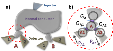
Figure 1: a) A normal conductor is connected to an injector biased at voltage $V$ and two detector nodes $A$ and $B$. The node $A$ ($B$) is coupled to grounded ferromagnetic detector terminals $A1$ and $A2$ ($B1$ and $B2$). b) Node $A$ is connected to the normal conductor, as well as nodes $A1$ and $A2$ via tunnel conductances $G_{A}$, $G_{A1}$, and $G_{A2}$, respectively. The polarizations $\mathbf{P}_{A1}$ and $\mathbf{P}_{A2}$ of the contacts to the ferromagnetic terminals are in opposite directions.

Let us first summarize and explain our main results i) and ii) for the non-local correlated spin transport properties in the device in Fig. 1: First, combining scattering theory and a Boltzmann-Langevin approach we derive an expression for the current correlations $S_{AiBj}=(2e^{2}/h)\int_{0}^{eV}dEs_{AiBj}(E)$ with

$$s_{AiBj}=4G_{Ai}G_{Bj}\langle(\delta f_{A}^{c}+\mathbf{P}_{Ai}\cdot\delta\mathbf{f}_{A})(\delta f_{B}^{c}+\mathbf{P}_{Bj}\cdot\delta\mathbf{f}_{B})\rangle_{f},$$ (1)

where $\mathbf{P}_{Ai}~{}(\mathbf{P}_{Bj})$ is the polarization of the tunnel contact to terminal $Ai$ ($Bj$), $\delta\hat{f}_{A/B}=\delta f_{A/B}^{c}\hat{1}+\delta\mathbf{f}_{A/B}\cdot\hat{\bm{\sigma}}$ is the fluctuating part of the $2\times 2$ spin distribution matrix at $A/B$, $\hat{\bm{\sigma}}=[\hat{\sigma}_{x},\hat{\sigma}_{y},\hat{\sigma}_{z}]$ is a vector of Pauli matrices, and $\langle..\rangle_{f}$ denotes the average over fluctuations. The matrix $\delta\hat{f}_{AB}$, with elements $\delta f_{AB}^{pq}=\langle\delta f_{A}^{p}\delta f_{B}^{q}\rangle_{f}$,  $p,q\in\{c,x,y,z\}$, is the spin correlation matrix, describing the irreducible, or exchange, correlations between spins at A and B.

We then show our result ii): $\delta\hat{f}_{AB}$ can be reconstructed by a sequence of measurements of e.g. $S_{A1B1}$ with different settings of $\mathbf{P}_{A1}$ and $\mathbf{P}_{B1}$. Importantly, this quantum spin tomography can be performed for arbitrary (finite) magnitudes of the polarizations $|\mathbf{P}_{A1}|$ and $|\mathbf{P}_{B1}|$ and spin-flip scattering in the conductor. Moreover, global spin symmetries limit the number of finite elements of $\delta\hat{f}_{AB}$, allowing for a simplified quantum spin tomography with fewer cross correlation measurements.

For a normal injector we derive a generic expression for $\delta\hat{f}_{AB}$, with nonzero elements

$$\delta f_{AB}^{cc}=\delta f_{AB}^{0}/2,\hskip 7.11317pt\delta f_{AB}^{xx}=\delta f_{AB}^{yy}=\delta f_{AB}^{zz}=\gamma\delta f_{AB}^{0}/2,$$ (2)

where $\delta f_{AB}^{0}$ is the equal-spin correlator and $\gamma$ quantifies the spin coherence in the conductor. $\gamma=1$ for a coherent system, $i.e.$ no spin-flip scattering, and $\gamma=0$ for a system with strong spin-flip relaxation. For a ferromagnetic injector, the correlations depend on the properties of the conductor, as shown below.

Inserting Eq. (2) into (1) gives a cross correlator

$$s_{AiBj}=2G_{Ai}G_{Bj}\delta f_{AB}^{0}[1+\gamma\mathbf{P}_{Ai}\cdot\mathbf{P}_{Bj}],$$ (3)

depending on the relative orientation of the polarizations $\mathbf{P}_{Ai}$ and $\mathbf{P}_{Bj}$. This together with Eq. (2) demonstrate our counter-intuitive result i): any conductor with a normal injector displays strong and universal non-local spin-correlations. We note that for the current cross correlator, similar results have been obtained in particular geometries Rev1 ; dilorenzo ; morten with no spin-flip scattering, $\gamma=1$.

We now describe the quantum spin tomography, starting for clarity with the known properties Brataas of the average spin distribution matrix in node $A$, $\hat{f}_{A}=f_{A}^{c}\hat{1}+\mathbf{f}_{A}\cdot\hat{\bm{\sigma}}$, where the real polarization vector $\mathbf{f}_{A}=[f_{A}^{x},f_{A}^{y},f_{A}^{z}]$ with $|\mathbf{f}_{A}|\leq 1$. The average current is $I_{A1}=(e/h)\int_{0}^{eV}dEi_{A1}(E)$ with Brataas

$$i_{A1}=2G_{A1}\left[f_{A}^{c}+\mathbf{P}_{A1}\cdot\mathbf{f}_{A}\right].$$ (4)

For the quantum spin tomography, we transform the orbital scheme developed in Ref. tomo to the spin degree of freedom and extend it to account for arbitrary detector polarization. Formally, to determine $f_{A}^{c},\mathbf{f}_{A}$ four independent measurements of the current are needed. The theoretically most convenient set $\{I_{A1}^{(k)}\}$, $k=1-4$ has the polarizations $\mathbf{P}_{A1}^{(1)}/P_{A1}=[0,0,1],\mathbf{P}_{A1}^{(2)}/P_{A1}=[0,0,-1],\mathbf{P}_{A1}^{(3)}/P_{A1}=[1,0,0]$ and $\mathbf{P}_{A1}^{(4)}/P_{A1}=[0,1,0]$, where $P_{A1}=|\mathbf{P}_{A1}|$, but other settings are also feasible. The expression in Eq. (4) then allows writing ($\{k\}=\{c,x,y,z\}$)

$$f_{A}^{k}=\frac{\sum_{l=1}^{4}Q^{kl}_{A1}I_{A1}^{(j)}}{4G_{A1}e^{2}V/h},\hskip 5.69046pt\frac{Q_{A1}}{P_{A1}}=\left(\begin{array}[]{cccc}P_{A1}^{-1}&P_{A1}^{-1}&0&0\\ -1&-1&2&0\\ -1&-1&0&2\\ 1&-1&0&0\end{array}\right)$$ (5)

Knowing the polarization $P_{A1}$ and the conductance $G_{A1}$ from independent measurements, the spin-distribution matrix $\hat{f}_{A}$ is fully reconstructed by current measurements. Importantly, for a normal injector, only $f_{A}^{c}$ is non-zero. For a ferromagnetic injector, when the spin quantization axis along the direction of polarization, only $f_{A}^{c}$ and $f_{A}^{z}$ are non-zero.

We then turn to the spin correlation matrix $\delta\hat{f}_{AB}$, with the 16 real elements $\delta f_{AB}^{pq}$. This implies that we need 16 independent cross correlator measurements to determine all elements $\delta f_{AB}^{pq}$ and reconstruct $\delta\hat{f}_{AB}$. From Eq. (1) we obtain the formal relation between the coefficients $\delta f_{AB}^{pq}$ and the cross correlators

$$\delta f_{AB}^{pq}=\frac{1}{8G_{A1}G_{B1}Ve^{3}/h}\sum_{k,l=1}^{4}Q_{A1}^{pk}Q_{B1}^{ql}S_{A1B1}^{(k,l)},$$ (6)

where $S_{A1B1}^{(k,l)}$ is the cross correlator with the detector terminal setting $k$ at $A1$ and $l$ at $B1$. Here $Q_{B1}$ is obtained from $Q_{A1}$ by changing $P_{A1}$ to $P_{B1}$.

For a normal injector, the requirement Been of invariance of $\delta\hat{f}_{AB}$ under any global spin rotation means that there is only four non-zero elements $\delta f_{AB}^{cc}$ and $\delta f_{AB}^{xx}=\delta f_{AB}^{yy}=\delta f_{AB}^{zz}$. For a ferromagnetic injector (defining the spin quantization axis) invariance of $\delta\hat{f}_{AB}$ under the global rotation $\{|\!\!\uparrow\rangle,|\!\!\downarrow\rangle\}\rightarrow\{e^{i\phi}|\!\!\uparrow\rangle,e^{-i\phi}|\!\!\downarrow\rangle\}$ yields Wang six non-zero elements $\delta f_{AB}^{cc},\delta f_{AB}^{cz},\delta f_{AB}^{zc},\delta f_{AB}^{zz}$ and $\delta f_{AB}^{xx}=\delta f_{AB}^{yy}$.

From Eqs. (5) and (6) the detector polarization settings necessary to determine the non-zero components of $\hat{f}_{A}$ and $\delta\hat{f}_{AB}$ are found: For a normal injector, only collinear polarizations at A and B are needed for both $\hat{f}_{A}$ and $\delta\hat{f}_{AB}$. For a ferromagnetic injector, for $\hat{f}_{A}$ the detector polarizations in addition have to be collinear with the injector one. However, for $\delta\hat{f}_{AB}$ non-collinear polarizations at A and B are necessary, e.g. both along the x and z axis, since $\delta f_{AB}^{zz}\neq\delta f_{AB}^{xx}=\delta f_{AB}^{yy}$. Importantly, for an unknown direction of the injector polarization or two (or more) non-collinear ferromagnetic injectors, the full tomographic scheme with detector polarizations along all three axes x,y and z are required.

We will now detail our calculations, assumptions, and approximations. In addition to the information given above, the normal conductor in Fig. 1 is connected to detector nodes $A$ and $B$ via tunnel barriers with conductances $G_{A}$ and $G_{B}$. The two ferromagnetic terminals $A1$ and $A2$  ($B1$ and $B2$) have opposite directions of polarization. We assume the limit of low temperature $kT\ll eV$. All conductances are much larger than unity.

It is assumed that the normal conductor consists of diffusive and/or chaotic parts, allowing a semiclassical treatment of the orbital properties. In contrast, spin is treated fully quantum mechanically. Furthermore, scattering is elastic. Following the magnetoelectronic circuit theory of Ref. Brataas , we discretize the system into nodes connected via tunnel barriers, see Fig. 1. Each node $\nu$, spatially much smaller than the spin-flip length, is characterized by a $2\times 2$ distribution matrix with an average, $\hat{f}_{\nu}$, and a fluctuating, $\delta\hat{f}_{\nu}$, part. To ensure that the detectors do not influence the spin-properties of the system, we require i) $G_{A}\ll G_{A1}+G_{A2}$ and $G_{B}\ll G_{B1}+G_{B2}$ so that an electron entering e.g. node $A$ from the conductor is emitted into $A1$ or $A2$ and do not return to the conductor and ii) $G_{A1}\mathbf{P}_{A1}=-G_{A2}\mathbf{P}_{A2}$ and $G_{B1}\mathbf{P}_{B1}=-G_{B2}\mathbf{P}_{B2}$, which ensures that no spin polarization is induced into the conductor from the ferromagnetic terminals, i.e. the measured spin signal arises from the conductor exclusively and not from the detector circuits.

Deriving Eqs. (4) and (1), we first review Brataas the spin information present in the average spectral current $i_{A1}(E)$. In the scattering approach Butrev , with no particles incident from terminal $A1$ in the bias window ($0\leq E\leq eV$), the spectral current is

$$i_{A1}=\sum_{n\sigma}\langle n_{A1,n}^{\sigma}\rangle,\hskip 14.22636ptn_{A1,n}^{\sigma}=b_{A1,n}^{\sigma\dagger}b_{A1,n}^{\sigma}$$ (7)

where $b_{A1,n}^{\sigma\dagger}$ creates an electron on the ferromagnetic side in the contact between $A1$ and $A$, in conduction mode $n$ propagating into $A1$ and the energy-dependence is suppressed. The spin quantization axis $\sigma=\uparrow,\downarrow$ is along the direction of $\mathbf{P}_{A1}$. The creation operators $b_{A1,n}^{\sigma\dagger}$ are related to the operators $b_{Am}^{\tau\dagger}$ for electrons on the normal conductor side, emitted from node $A$ towards $A1$, via the spin-dependent transmission matrix of the normal-ferromagnetic interface $t_{A1}$ with elements $t_{A1,nm}^{\sigma\tau}$. Following Ref. Brataas , we make the semiclassical approximation that the spin distribution matrix in node $A$ is independent on mode index, i.e. $\langle b_{An}^{\sigma\dagger}b_{Am}^{\sigma^{\prime}}\rangle=\hat{f}_{A}^{\sigma\sigma^{\prime}}\delta_{nm}$, giving

$$i_{A1}=\sum_{\sigma\tau}\hat{\mathcal{T}}_{A1}^{\tau\sigma}\hat{f}_{A}^{\sigma\tau}=G_{A1}\mbox{tr}\left\{(\hat{1}+\mathbf{P}_{A1}\cdot\hat{\bm{\sigma}})\hat{f}_{A}\right\}\,.$$ (8)

Here Brataas $\hat{\mathcal{T}}_{A1}=\sum_{nm}(\hat{t}_{A1,nm})^{T}(\hat{t}_{A1,nm})^{*}=G_{A1}(\hat{1}+\mathbf{P}_{A1}\cdot\hat{\bm{\sigma}})$ where the elements of the $2\times 2$ matrix are $(\hat{t}_{A1,nm})_{\sigma\tau}=t_{A1,nm}^{\sigma\tau}$. Eq. (8) directly gives Eq. (4). Similar relations hold for the average currents into $A2$, $B1$ and $B2$.

We then turn to the low frequency correlations between electrical currents in e.g. terminals $A1$ and $B1$, $S_{A1B1}=\int dt\langle\Delta I_{A1}(0)\Delta I_{B1}(t)\rangle$. Scattering theory Butrev gives

$$s_{A1B1}=\sum_{nm,\sigma\tau}\left[\langle n_{A1,n}^{\sigma}n_{B1,m}^{\tau}\rangle-\langle n_{A1,n}^{\sigma}\rangle\langle n_{B1,m}^{\tau}\rangle\right]$$ (9)

where $n_{B1,m}^{\tau}=b_{B1,m}^{\tau\dagger}b_{B1,m}^{\tau}$ and $b_{B1,m}^{\tau\dagger}$ creates an outgoing electron on the ferromagnetic side, in conduction mode $m$ in $B1$ with spin quantization axis along the direction of the magnetization $\mathbf{n}_{B}$. Disregarding terms of second order in $G_{A}/(G_{A1}+G_{A2})$ or $G_{B}/(G_{B1}+G_{B2})$, the operators $b_{A1,n}^{\sigma\dagger}$ and $b_{B1,m}^{\tau\dagger}$ are expressed in terms of the operators $b_{Ak}^{\sigma^{\prime}\dagger}$ and $b_{Bl}^{\tau^{\prime}\dagger}$ and the scattering amplitudes of the respective normal-ferromagnetic interfaces. Making the semiclassical approximation that the non-local irreducible correlator $\langle b_{An}^{\sigma\dagger}b_{Am}^{\sigma^{\prime}}b_{Bk}^{\tau\dagger}b_{Bl}^{\tau^{\prime}}\rangle-\langle b_{An}^{\sigma\dagger}b_{Am}^{\sigma^{\prime}}\rangle\langle b_{Bk}^{\tau\dagger}b_{Bl}^{\tau^{\prime}}\rangle\equiv\delta\hat{f}_{AB}^{\sigma\sigma^{\prime},\tau\tau^{\prime}}\delta_{nm}\delta_{kl}$, we arrive at

$$s_{A1B1}=\sum_{\sigma\sigma^{\prime}\tau\tau^{\prime}}\hat{\mathcal{T}}_{A1}^{\sigma^{\prime}\sigma}\hat{\mathcal{T}}_{B1}^{\tau^{\prime}\tau}\hat{f}_{AB}^{\sigma\sigma^{\prime},\tau\tau^{\prime}}=G_{A1}G_{B1}$$ (10)

$$\times \mbox{tr}\left\{\left[\left(\hat{1}+\mathbf{P}_{A1}\cdot\hat{\bm{\sigma}}\right)\otimes\left(\hat{1}+\mathbf{P}_{B1}\cdot\hat{\bm{\sigma}}\right)\right]\delta\hat{f}_{AB}\right\}$$

where $\hat{\mathcal{T}}_{B1}$ is obtained by changing all indices $A$ to $B$ in $\hat{\mathcal{T}}_{A1}$ and $\otimes$ is the tensor product. Here we work in the basis $\{|\sigma\tau\rangle\}=[|\!\uparrow\uparrow\rangle,|\!\uparrow\downarrow\rangle,|\!\downarrow\uparrow\rangle,|\!\downarrow\downarrow\rangle]$, i.e. the matrix elements $(\delta\hat{f}_{AB})_{|\sigma\tau\rangle,|\sigma^{\prime}\tau^{\prime}\rangle}=\delta\hat{f}_{AB}^{\sigma\sigma^{\prime},\tau\tau^{\prime}}$. As is shown below, the $4\times 4$ spin correlation matrix $\delta\hat{f}_{AB}=\langle\delta\hat{f}_{A}\otimes\delta\hat{f}_{B}\rangle_{f}$, provides a semiclassical interpretation of $\delta\hat{f}_{AB}$. This means that Eq. (10) directly gives Eq. (1). Moreover, the expressions for the other correlators $S_{AiBj}$ can similarly be given in terms of $\delta\hat{f}_{AB}$. This shows that $\delta\hat{f}_{AB}$ contains all information about non-local spin-correlations that can be obtained from cross correlations.

To further investigate the properties of $\hat{f}_{A},\hat{f}_{B}$ and $\delta\hat{f}_{AB}$ we now turn to the spin-dependent Boltzmann-Langevin approach of Ref. Arne . The average part of the distribution matrix $\hat{f}_{\nu}$ at node $\nu$ is determined from the condition of conservation of matrix currents into the node, $\sum_{\mu}\hat{i}_{\nu\mu}=0$, $i_{\nu\mu}=-i_{\mu\nu}$. The $2\times 2$ matrix current between a normal node $\nu$ and a ferromagnetic or normal node $\mu$ is $\hat{i}_{\nu\mu}=(G_{\nu\mu}/2)\left\{(\hat{1}+\mathbf{P}_{\mu}\cdot\hat{\bm{\sigma}}),(\hat{f}_{\nu}-\hat{f}_{\mu})\right\}$ with $\{.,.\}$ the anti-commutator, $G_{\nu\mu}$ the tunnel conductance between the nodes and $\mathbf{P}_{\mu}$ the polarization vector of node $\mu$ ($\mathbf{P}_{\mu}=0$ for a normal node). The distribution matrices for normal and ferromagnetic terminal nodes are $\hat{1}$ for biased terminals and $0$ for grounded. This allow us to calculate the distribution matrices of all nodes.

For the fluctuating part of the distribution matrix, we first note that the total fluctuations of the matrix current $\Delta\hat{i}_{\nu\mu}$ flowing between two nodes $\nu$ and $\mu$ is a sum of the bare fluctuations $\delta\hat{i}_{\nu\mu}$ and $\delta\hat{\mathcal{I}}_{\nu\mu}$ due to the fluctuating distribution matrices. For $\nu$ normal and $\mu$ normal or ferromagnetic $\delta\hat{\mathcal{I}}_{\nu\mu}=(G_{\nu\mu}/2)\left\{(\hat{1}+\mathbf{P}_{\mu}\cdot\hat{\bm{\sigma}}),(\delta\hat{f}_{\nu}-\delta\hat{f}_{\mu})\right\}$. The requirement of matrix current fluctuation conservation $\sum_{\mu}\Delta\hat{i}_{\nu\mu}=0$ then gives $\delta\hat{f}_{\nu}$ in terms of $\delta\hat{i}_{\nu\mu}$. The bare fluctuations $\delta\hat{i}_{\nu\mu}$ at different contacts are uncorrelated while for $\nu,\mu$ normal $\langle\delta\hat{i}_{\nu\mu}\otimes\delta\hat{i}_{\nu\mu}\rangle_{f}=(G_{\nu\mu}/2)\left[\hat{f}_{\nu}\otimes(\hat{1}-\hat{f}_{\mu})+\hat{f}_{\mu}\otimes(\hat{1}-\hat{f}_{\nu})\right]\hat{W}+h.c.$ where $h.c.$ denote hermitian conjugate and the permutation matrix $\hat{W}$ has nonzero elements $W_{11}=W_{23}=W_{32}=W_{44}=1$. For $\nu$ normal and $\mu$ ferromagnetic we have $\langle\delta\hat{i}_{\nu\mu}\otimes\delta\hat{i}_{\nu\mu}\rangle_{f}=(G_{\nu\mu}/2)\{([\hat{1}+\mathbf{P}_{\mu}\cdot\hat{\bm{\sigma}}]f_{\mu})\otimes(\hat{1}-\hat{f}_{\nu})+([\hat{1}+\mathbf{P}_{\mu}\cdot\hat{\bm{\sigma}}][1-f_{\mu}])\otimes\hat{f}_{\nu}\}\hat{W}+h.c.$. Here we used that ferromagnetic (i.e. terminal) distributions do not fluctuate. From these relations any electrical current correlator $\langle\Delta i_{\nu}\Delta i_{\mu}\rangle_{f}$, with $\Delta i_{\nu}=\mbox{tr}[\Delta\hat{i}_{\nu}]$, can be obtained.

Spin flip scattering is taken into account on the level of the relaxation time approximation. This amounts to coupling each node $n$ to a spin-flip node $\varphi\nu$ with a tunnel contact with conductance $G_{\varphi\nu}\propto 1/\tau_{\varphi\nu}$, with $\tau_{\varphi\nu}$ the spin-flip time of the node, and requiring conservation of electrical current and current fluctuations into the spin-flip node. Here we give the universal results of the calculation, i.e. we consider an arbitrary normal conductor with any amount of (spatially dependent) spin-flip scattering, the details of the calculations are given elsewhere. First, by comparing the obtained expression for the spectral cross correlators $s_{AiBj}=\langle\Delta i_{A1}\Delta i_{B1}\rangle_{f}$ with Eq. (10) we conclude that $\delta\hat{f}_{AB}=\langle\delta\hat{f}_{A}\otimes\delta\hat{f}_{B}\rangle_{f}$, discussed above. Second, for normal injectors, we find the generic form

$$\delta\hat{f}_{AB}=(\delta f_{AB}^{0}/2)\left[(1-\gamma)\hat{1}\otimes\hat{1}+2\gamma\hat{W}\right]$$ (11)

This is just the result in Eq. (2).

Further insight is obtained by calculating the properties of the simplest possible conductor, a single node spindot . For a normal injector we find the distribution function at e.g. A as $\hat{f}_{A}=G_{A}/(G_{A1}+G_{A2})f\hat{1}$, with $f=G/(G+G_{A}+G_{B})$ the distribution function of the conductor node and $G$ the injector-conductor node conductance. This is independent on spin-flip scattering. For the spin-correlation matrix we get the result in Eq. (11) with $\delta f_{AB}^{0}=f^{3}G_{A}G_{B}/[G(G_{A1}+G_{A2})(G_{B1}+G_{B2})]$ and $\gamma=[1+\tau/\tau_{\varphi}]^{-1}$ with $\tau/\tau_{\varphi}=G_{\varphi}/(G_{A}+G_{B}+G)$ the ratio of spin-flip and dwell times in the central node.

For a ferromagnetic injector with polarization $\mathbf{P}_{I}$ the spin distribution matrix at e.g. A has two non-zero components $(\hat{f}_{A})^{\uparrow\uparrow}\equiv f_{A}^{\uparrow}$ and $(\hat{f}_{A})^{\downarrow\downarrow}\equiv f_{A}^{\downarrow}$ with $f_{A}^{\uparrow,\downarrow}=f[(1\pm P_{I})(1\mp P_{I}f)+\tau_{\varphi}/\tau]/[(1-P_{I}^{2}f^{2})+\tau_{\varphi}/\tau]$ with $P_{I}=|\mathbf{P}_{I}|$. For the spin-correlation matrix, the full expression, including spin-flip scattering, becomes very lengthy and we only present the result for $\gamma=1$. This is $\delta f_{AB}^{cc}=\delta f_{AB}^{zz}=\delta f_{AB}^{0}(c_{+}+c_{-})/2$, $\delta f_{AB}^{cz}=\delta f_{AB}^{zc}=\delta\delta f_{AB}^{0}(c_{+}-c_{-})/2$ and $\delta f_{AB}^{xx}=\delta f_{AB}^{yy}=\delta f_{AB}^{0}c_{0}/2$ with $c_{\pm}=(1\pm P_{I})^{2}/(1\pm P_{I}f)^{3}$ and $c_{0}=(1-P_{I}^{2})/[1-(P_{I}f)^{2}]$. Inserting this into Eq. (10) we get the cross correlator

$$S_{A1B1}=2G_{A1}G_{A1}\delta f_{AB}^{0}(c_{I}+c_{0}[1+\mathbf{P}_{A1}\cdot\mathbf{P}_{B1}])$$ (12)

with $c_{I}=(1+P_{A1}^{z}P_{B1}^{z})(c_{+}+c_{-}-2c_{0})/2+(P_{A1}^{z}+P_{B1}^{z})(c_{+}-c_{-})/2$. This clearly demonstrates that while a ferromagnetic injector leads to a polarization of the conductor, it suppresses the spin-correlations.

In conclusion we have presented a scheme for quantum state tomography of non-local spin correlations in normal-ferromagnetic conductors. Non-local correlations are generically strong but suppressed by spin-flip scattering and ferromagnetic injectors.

We acknowledge discussions with Daniel Huertas Hernando. This work was supported by the Swedish VR and the Research Council of Norway, Grant No 162742/V00.

References

(1) Y. Ohno et al, Nature 402 790 (1999);
R. Fiederling et al, Nature 402 787 (1999); F. J. Jedema,
A. T. Filip, B. J. van Wees, Nature 410 345, (2001); F. J. Jedema
et al, Nature 416 713 (2002).
(2) M. Zaffalon, and B. J. van Wees, Phys. Rev. Lett, 91 186601, (2003).
(3) M. Johnson, R. H. Silsbee, Phys. Rev. B 37 5312
(1988); Phys. Rev. B 37 5326 (1988).
(4) H.-A. Engel, E. I. Rashba, and B. I. Halperin, arXiv:0603306.
(5) D. C. Ralph and M. D. Stiles, J. Magn. Magn. Mater.
320, 1190 (2008).
(6) Y. Tserkovnyak et al, Rev. Mod. Phys. 77
, 1375 (2005).
(7) S. Datta, and B. Das, Appl. Phys. Lett. 56 665
(1990); K. Ono et al, J. Phys. Soc. Jpn. 65 3449 (1996);
G. E. W. Bauer et al Appl. Phys. Lett. 82 3928 (2003).
(8) F. S. Bergeret, A. F. Volkov, and K. B. Efetov, Rev. Mod. Phys.
77, 1321 (2005).
(9) B. R. Bulka et al, Phys. Rev. B 60, 12246
(1999); R. Lopez, and D. Sanchez, Phys. Rev. Lett. 90,
116602 (2003); F. M. Souza, A. P. Jauho, J. C. Egues, Phys. Rev. B 78, 155303 (2008).
(10) E.R. Nowak, M. B. Weissman, and S. S. S. Parkin, App. Phys.
Lett. 74, 600 (1999); E. G. Mishchenko, Phys. Rev. B 68, 100409(R) (2003); A. Lamacraft, Phys. Rev. B 69, 081301(R) (2004); E.G. Mishchenko, A. Brataas, and Y. Tserkovnyak, Phys.
Rev. B 69, 073305 (2004); R. Guerrero et al. Phys. Rev. Lett. 97, 266602 (2006).
(11) Y. Tserkovnyak and A. Brataas, Phys. Rev. B. 64
214402 (2001).
(12) A. Cottet, W. Belzig, and C. Bruder, Phys. Rev. Lett.
92, 206801 (2004); Phys. Rev. B.
70, 115315 (2004); O. Sauret and D. Feinberg, Phys. Rev. Lett. 92,
106601 (2004); D. Sanchez, and R. Lopez, Phys. Rev. B 71, 035315 (2005).
(13) W. Belzig, and M. Zareyan, Phys. Rev. B 69,
140407(R) (2004); M. Zareyan, and W. Belzig, Phys. Rev. B 71,
184403 (2005).
(14)
F. Taddei, and R. Fazio, Phys. Rev. B 65, 134522 (2002).
(15) D. Sanchez et al, Phys. Rev. B 68, 214501
(2003).
(16) S. Kawabata, J. Phys. Soc. Jpn. 70 1210 (2001);
N. Chtchelkatchev et al, Phys. Rev. B, 66,
161320(R) (2002).
(17) A. Di Lorenzo and Yu. V. Nazarov, Phys. Rev. Lett.
94, 210601 (2005).
(18) J. P. Morten et al, Europhys. Lett. 81 40002 (2008).
(19) A. Brataas, Yu. V. Nazarov, and G. E. W. Bauer, Phys. Rev.
Lett. 84, 2481 (2000); Eur. Phys. J. B 22, 99 (2001).
(20) M. Büttiker, Phys. Rev. B 46, 12485 (1992); Ya.
Blanter and M. Büttiker, Phys. Rep. 336, 1 (2000).
(21) P. Samuelsson, M. Büttiker, Phys. Rev. B, 73,
041305(R) (2006).
(22) B. Michaelis, and C.W.J. Beenakker, Phys. Rev. B, 73
, 115329 (2006).
(23) X. Wang, and P. Zanardi, Phys. Lett. A 301 1 (2002).