Scale invariant properties of public debt growth

Abstract

Public debt is one of the important economic variables that quantitatively describes a nation’s economy. Because bankruptcy is a risk faced even by institutions as large as governments (e.g. Iceland), national debt should be strictly controlled with respect to national wealth. Also, the problem of eliminating extreme poverty in the world is closely connected to the study of extremely poor debtor nations. We analyze the time evolution of national public debt and find “convergence”: initially less-indebted countries increase their debt more quickly than initially more-indebted countries. We also analyze the public debt-to-GDP ratio ${\cal R}$, a proxy for default risk, and approximate the probability density function $P({\cal R})$ with a Gamma distribution, which can be used to establish thresholds for sustainable debt. We also observe “convergence” in ${\cal R}$: countries with initially small ${\cal R}$ increase their ${\cal R}$ more quickly than countries with initially large ${\cal R}$. The scaling relationships for debt and ${\cal R}$ have practical applications, e.g. the Maastricht Treaty requires members of the European Monetary Union to maintain ${\cal R}<0.6$.

I Introduction

Just as an individual is expected to control his/her debt to asset ratio, so is a government expected to control its national debt as a function of the country’s wealth, measured e.g. by its gross domestic product (GDP). In a dynamic global economy, excessive borrowing cannot persist indefinitely, as creditors are bound to call in large loans. While a country suffers financial problems when its GDP does not increase fast enough, even more serious trouble begins when its debt increases faster than its GDP. While national GDP has been the topic of many studies on economic growth barro91 ; Levine92 ; Durlauf96 ; barrobook , the empirical analysis of public debt has lagged due to lack of comprehensive data.

Large sets of public debt data, dating back several decades, and ranging from poor to rich countries, have recently become available. Here we use concepts of statistical physics to analyze public debt data for a wide cross-section of economies including underdeveloped, developing, and developed countries. The total public debt data, along with total GDP data, are available at the Inter-American Development Bank data0 , and are compiled and analyzed in Refs. JP06a ; JP06b . Population data are available by the World Bank, and can be reconstructed through GDP and per capita GDP data compiled in Ref. data1 . We deflate all USD amounts to in units of the USD in the year 2000 data2 . In our analysis, we compare public debt only within the same country, in order to avoid any differences in the theoretical and practical definition of debt and the reporting of debt by various countries, an issue pointed out in Refs. JP06a ; JP06b ; kotlikoff . Our results are robust with respect to mis-reporting and ambiguous definitions of public debt kotlikoff . In Fig. 1 we plot the debt-to-GDP ratio ${\cal R}$ for many countries, grouped in panels (a-d) by common historical, geographical, and financial factors. In Fig. 1(d) we plot the average debt-to-GDP ratio for three subgroups corresponding to World Bank Income Group (IG) classifications, and observe relatively high levels of ${\cal R}$ among the poorest countries.

Economic growth theories predict that GDP should “converge” towards equality, with wealthy countries experiencing smaller relative growth rates than poor countries. However, the opposite has been found for economic wealth data barromartin91 ; barromartin92 ; martin96 . So we address the question, what are the growth dynamics for public debt? To answer this question, we analyze a comprehensive database of national public debt and GDP to investigate the dynamics of debt growth and growth in ${\cal R}$.

With the current global credit crunch, and several notable recent national defaults, it is important to address sustainable public debt, defined as the amount of debt where the receiving country is capable of meeting its current and future debt obligations reinhart ; kraay . The total current government debt $D(t)$ increases from last year’s debt $D(t-1)$ partially due to interest payments on the debt $D(t-1)$ at interest rate $I_{D}(t)$, and partially because of the current primary deficit, defined as the difference between spending $S(t+1)$ and taxes $T(t+1)$ blanchard85 . Thus

$$D(t)=[1+I_{D}(t-1)]D(t-1)+[S(t)-T(t)]\ .$$ (1)

We consider three possible scenarios for public debt growth dynamics:

• Growth rates of the country debt do not depend on the initial debt level.

• A more indebted country has a larger debt growth rate than a less indebted country, so that relative differences between debt across countries increases over time (divergence).

• A more indebted country has a smaller debt growth rate than a less indebted country, so that relative differences between debt across countries decreases over time (convergence).

These three scenarios have different implications for investors, who will only accept government debt up to some ceiling. Hence, one would expect that more indebted countries would increase their debt more slowly than less indebted countries.

II Empirical results

To ascertain which of the three debt scenarios is better supported by empirical facts, we define for country $i$ the annualized logarithmic growth rate of per capita initial debt $d_{i}(t)$ between years $t$ and $t+\Delta t$

$$r_{i}(t,t+\Delta t)\equiv\frac{\log[d_{i}(t+\Delta t)/d_{i}(t)]}{\Delta t}\ .$$ (2)

We compare $r_{i}(t,t+\Delta t)$ to $d_{i}(t)$, assuming $r_{i}(t,t+\Delta t)$ depends on debt size by

$$r_{i}(t,t+\Delta t)\cong\alpha-\beta~{}\log[d_{i}(t)]\ .$$ (3)

The functional form of Eq. (3) can also be expressed as

$$\log[d_{i}(t+\Delta t)]=\alpha~{}\Delta t+(1-\beta\Delta t)\log[d_{i}(t)]$$ (4)

If $\beta>0$, there is convergence in per capita debt data across countries, since initially more indebted economies tend to increase their debt slower (smaller $r_{i}(t,t+\Delta t)$) than initially less indebted economies. Hence, $\beta$ represents the “speed of convergence”, a concept introduced for per capita GDP data in Ref. martin96 . A larger positive value of $\beta$ results in faster convergence, equalizing the per capita debt across all countries more quickly. If $\beta<0$ there is divergence in debt data, where initially less-indebted countries with smaller $d_{i}(t)$ increase their debt slower than initially more-indebted countries.

In Fig. 2 we plot the 1990 per capita debt of more than 80 countries, representing low-, medium-, and high-wealth countries, considering several relationships. First, we compare the per capita debt over (a) 15-year and (d) 7-year time horizons. We find the slope $S=(1-\beta\Delta t)$ of the regression in Eq. (4) is less than one, requiring $\beta>0$ which corresponds to scenario (iii).

To confirm the convergence across countries for other time horizons, Fig. 3 shows the value of $S$ for varying initial $d(t)$ and time horizon $\Delta t$ in Eq.(4). We find $S\equiv 1-\beta\Delta t<1$ for most horizons $\Delta t$, implying convergence, where less-indebted countries increase their debt faster than more-indebted countries. However, there is a period in the beginning of the 1990’s that is the exception, with $S>1$ and $\beta<0$. This period of divergence in per capita debt may be related to the 20-year lows in interest rates which may have resulted in increased borrowing, even among heavily indebted countries. Since 1995, the values of $S$ have returned to values less than one, indicating a return to convergence.

We also analyze the growth rates of per capita GDP and confirm the divergence across countries observed originally in barromartin91 ; barromartin92 ; martin96 . In Fig. 4 we plot for per capita GDP, the analogous regression $S$ values that we plot in Fig. 3 for per capita public debt. For all periods $\Delta t$ and initial years analyzed, we find values of $S>1$ indicating divergence.

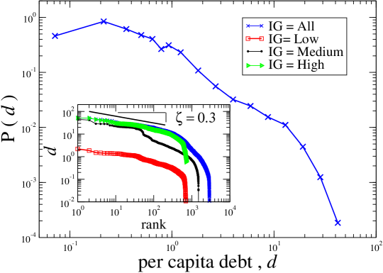
Figure 5: Right-skewed probability density function $P(d)$ of per capita debt $d$ for all countries analyzed over the 36-year period 1970-2005 in units of $10^{3}$ USD per person in the year 2000. (Inset) Zipf rank-frequency plot for $d$ values for all countries and for three subgroups according to World Bank Income Group (IG) classification. Countries in the high and medium IG categories contribute to the wide range of $d$ values, whereas poor countries have relatively small $d$ values reflecting their small per capita borrowing capacity. We also show a power-law with exponent $\zeta=0.3$ for comparison.

A natural question is – how does the per capita debt $d_{i}$ vary across all countries and by income group? Power law probability density functions (pdf) have been observed for total country GDP globalization2 and per capita GDP GDPpercapPDF . Fig. 5 shows the pdf $P(d)$ for all countries analyzed over the 36-year period 1970-2005. We observe large variations across income groups, where low income countries typically have relatively small per capita debt values reflecting their small per capita borrowing capacity. In contrast to the zipf-rank curves for GDP with $\zeta_{GDP}\approx 1$ corresponding to pdf scaling exponent exponent $1+1/\zeta_{GDP}\approx 2$globalization2 , we observe in Fig. 5(inset) a scaling value $\zeta_{d}\approx 0.3$ corresponding to a relatively large pdf scaling exponent $1+1/\zeta_{d}\approx 4.3$.

In a country where both GDP and debt grow with time, one must analyze the dynamics of both debt and GDP. Since a debt that is large for Luxembourg is not large for the U.S., various indices have been proposed in order to compare the burden of debt to the ability of the country’s economy to generate income. These include ${\cal R}$blans89 ; ecogrowth , so we apply the convergence analysis of Eq. (4) to ${\cal R}(t)$ obtaining

$$\log[{\cal R}_{i}(t+\Delta t)]=\alpha^{\prime}~{}\Delta t+(1-\beta^{\prime}\Delta t)\log[{\cal R}_{i}(t)]\ .$$ (5)

Fig. 2 compares ${\cal R}(t)$ over (b) 15-year and (e) 7-year time horizons. Fig. 7 shows $S^{\prime}\equiv(1-\beta^{\prime}\Delta t)<1$, implying convergence $\beta^{\prime}>0$, over a large range of $\Delta t$-year horizons for initial year $t$.

A responsible government is expected to monitor simultaneously the growth of debt and GDP blanchard94 . By borrowing money, a country may increase ${\cal R}(t)$ for some time, but clearly ${\cal R}(t)$ cannot increase indefinitely, as increased debt can negatively affect GDP growth saint . Banks prefer individuals with large incomes and small debts. Banks also prefer countries that have, for a given GDP level, small relative debt. Fig. 1 provides the annual trend of ${\cal R}(t)$ for several groups of countries with common geo-politial backgrounds.

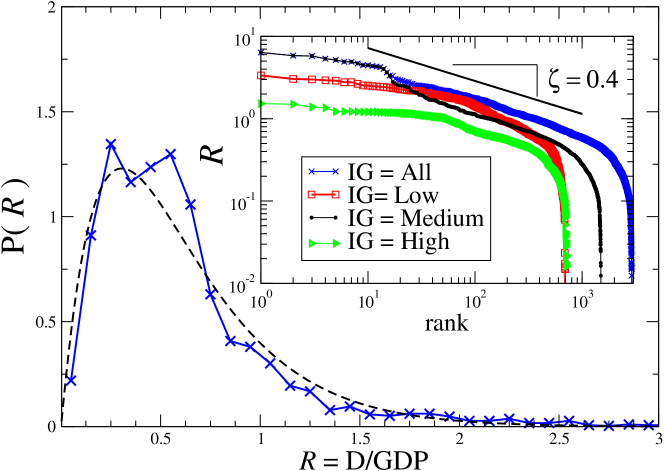
Figure 8: Probability density function $P({\cal R})$ for all countries analyzed over the 36-year period 1970-2005. For comparison, we approximate $P({\cal R})$ with a Gamma distribution with parameters $k=2.0$ and ${\cal R}_{c}=0.30$. The extreme statistics of $P({\cal R})$ can quantify the threshold of sustainable debt. (Inset) Zipf rank-frequency plot for ${\cal R}$ values. We separate data into three subgroups by World Bank Income Group (IG) classification to demonstrate the range of large ${\cal R}$ values within different wealth groups. The straight line is a power law with exponent $\zeta=0.4$ for comparison.

Debtor default risk is estimated by many rating agencies and financial organizations. ${\cal R}(t)$ is an important quantity for determining the ability of a debtor to make debt payments. For large ${\cal R}(t)$ there is a larger probability that the debtor will not be able to make timely payments or be able to prevent further debt increase with time, scenarios that lead to credit default. In order to quantify the risky debt levels, we collect the ${\cal R}(t)$ values of all countries analyzed over the 36-year period 1970-2005 and plot the pdf $P({\cal R})$ in Fig. 8. We find $<{\cal R}>=0.57\pm 0.54$, and we fit the pdf to a Gamma distribution $P({\cal R})\propto{\cal R}^{k-1}\exp[-{\cal R}/{\cal R}_{c}]$ with $k=2.0\pm 0.1$ and ${\cal R}_{c}=0.30\pm 0.01$, using the maximum likelihood estimator. The extreme value statistics of Gamma pdf can be used to define thresholds for sustainable debt.

In order to analyze the countries that have large ${\cal R}(t)$ and a high risk of default, the countries which constitute the pdf tail, we plot rank-frequency curves in Fig. 8(inset). The Zipf plots show a power law over three orders of magnitude, with scaling exponent $\zeta_{\cal R}\approx 0.4$ corresponding to $P({\cal R})\sim{\cal R}^{-3.5}$.

III Model

Our analysis, performed across a wide cross section of countries, confirms the existence of convergence in public debt. This is opposite of what is in GDP data barromartin91 ; barromartin92 ; martin96 , where the speed of convergence $\beta$ is negative. We now discuss how to model the scaling result we obtain, and how to use the scaling result obtained for GDP and public debt. Figs. 2(c) and 2(f) compare the per capita debt to per capita GDP for the years 1990 and 2005. The typical relationship between debt and GDP shows a scale invariant form,

$$g\sim A~{}d^{\gamma}\ ,$$ (6)

where $g$ is the per capita GDP and $d$ is the per capita debt. In Fig. 7 we plot the values of $\gamma$ for the set of countries analyzed in each yearly data set.

In order to model debt dynamics, we assume that the functional dependence in Eq. (6) is time invariant. Note that if $g(t)$ and $d(t)$ grow exponentially with different growth rates, $r_{g}$ and $r_{d}$, the relationship between $g(t)$ and $d(t)$ still has the form of a power law, with $r_{g}=\gamma\ r_{d}$.

We may consider the dynamics of public debt by assuming that the government borrows $B(t)$, a fixed proportion of GDP given by $B(t)\equiv D(t)-D(t-1)\equiv\Delta D(t)=b~{}G(t)$, with deficit ratio $b=$ constant brauninger . Then $r_{D}\equiv\Delta D/D=b~{}G(t)/D(t)$, and

$$r_{d}=b~{}g(t)/d(t)-r_{pop}=bN/d(t)^{1-\gamma}-r_{pop}\ ,$$ (7)

where $r_{pop}$ denotes the population growth rate ecogrowth . Hence,

$$\frac{\partial r_{d}}{\partial d}=\frac{-bN(1-\gamma)}{d^{2-\gamma}}\propto 1/d^{2-\gamma}\ .$$ (8)

We observe from Fig. 7 that $\gamma\lesssim 1$ so that $\partial r_{d}/\partial d\simeq-1/d$. For this reason, we use the regression $r_{d}\cong\alpha-\beta~{}\log[d_{i}(t)]$, which agrees well with the data in Figs. (2) and (3).

IV Discussion

In summary, we demonstrate convergence in per capita public debt across a wide set of countries during the period 1970-2005, a result of general interest for complex systems researchers as well as for creditors. Our analysis is made possible by new comprehensive data sets, and extends empirical surveys previously performed on country GDP which found divergence in country GDP. While divergence in country GDP implies that economic wealth is moving away from global equality, convergence in per capita debt implies that indebtedness is becoming an economic standard. Furthermore, convergence in the ${\cal R}$ implies that relative differences in indebtedness across countries is also decreasing over time. Some economists believe that convergence across all countries is possible through globalization globalization1 ; globalization2 ; globalization3 ; globalization4 and access to open markets SachsEconReform . While public debt can be used to invest in a country’s development via physical infrastructure, technology, and social programs, its use requires responsible governance. CorruptionCorruption1 ; Corruption2 and the misuse of public debt can lead to insurmountable debt contributing to financial crisis, which can cause further increase in debt levels through exchange rate depreciation bolle ; sachs88 . There are also instances of extremely poor debtor nations that are unable to meet their current and future debt obligations (See Fig. 1). Recent programs such as the Heavily Indebted Poor Countries (HIPC) Initiative, sponsored by the World Bank and the IMF, and the Jubilee 2000 Campaign-to-Drop-the-Dept, have called on debt cancellation for extremely poor debtor nations as a crucial step in the UN Millennium Project to eliminate extreme poverty SachsPoverty ; SachsPovertyAfr ; UNMilleniumProject . Further, debt has become a problem for not only the extremely poor countries. With the current global credit crunch, their is an increased need for responsible use of government debt.

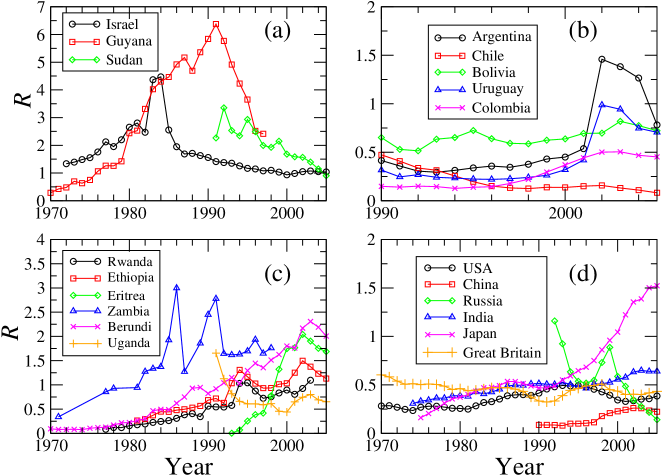
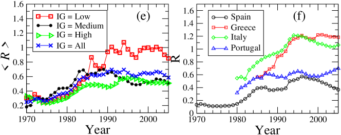
Figure 1: Illustration of debt-to-GDP ratio ${\cal R}(t)$ for (a-d) several countries and (e) the average trend for three subsets according to World Bank Income Group (IG) classifications. (a) Countries with turmoil, as in the case of Israel and Sudan which experienced periods of war, and Guyana which formed a new government, can experience periods of extremely high ${\cal R}$. (b) The Argentine financial crisis of the late 1990’s placed many South American countries in a state of debt stress. (c) The debt burden in many African countries, some which are also plagued by war and political turmoil, is increasing with time. Many of these countries are candidates for foreign debt cancellation (jubilee). (d) Several large countries. (e) The average ${\cal R}$ is increasing with time, with low-income countries currently at relatively high levels reflecting the burden of unsustainable debt. (f) Mediterranian countries with recent concern of default risk.

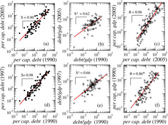
Figure 2: The 3 possible relations between per capita debt, per capita GDP, and ${\cal R}$ for a set of low-income, medium-income, and high-income countries. Regression of per capita debt $d(t)$ in 1990 versus per capita debt $d(t+\Delta t)$ for (a) $\Delta t=15$ years and (d) $\Delta t=7$ years later indicates that there is convergence in the per capita debt data across the countries over the larger time horizon in panel (a) with $S\equiv 1-\beta\Delta t<1$ implying $\beta>0$. Regression of ${\cal R}(t)$ in 1990 versus ${\cal R}(t+\Delta t)$ for (b) $\Delta t=$ 15 years and (e) $\Delta t=$ 7 years indicates that there is also convergence over these time horizons. (c,f) We also illustrate the scale invariant relation between between per capita debt and per capita GDP in units of $10^{3}$ USD per person in the year 2000.

Figure 3: The slope $S\equiv 1-\beta\Delta t$ of the log-log regression in Eq. (4) is typically less than one for a given time horizon of $\Delta t$ years after the initial year $t$ labeling each panel. Values of $S<1$ imply convergence ($\beta>0$) in per capita debt over the $\Delta t$-year period. $R^{2}$ values for log-log regressions are typically $>$ 0.7 for $10<\Delta t<20$ years, and are typically $>$ 0.8 for $1<\Delta t<10$ years, while the number of countries for each regression varies between 22-25 (1970) and 103-120 (1995). Interestingly, we observe a short period of divergence, where for initial years 1980 and 1985, the value of $S>1$ for $\Delta t\approx 12$ years corresponding to the mid-1990’s.

Figure 4: For comparison, we also analyze GDP growth rates and find divergence for all periods analyzed. The slope $S$ of the log-log regression in Eq. (4) for per capita GDP is typically greater than one for a given time horizon of $\Delta t$ years after the initial year, which we label in each panel. Values of $S>1$ imply divergence ($\beta<0$) in per capita GDP over the $\Delta t$-year period, consistent with the seminal work of barro91 ; martin96 .

Figure 6: The slope $S^{\prime}\equiv 1-\beta^{\prime}\Delta t$ of the log-log regression in Eq. (5) of ${\cal R}$. We find $S^{\prime}<1$ a given time horizon of $\Delta t$ years after the initial year $t$ labeling each panel. Values of $S<1$ imply convergence ($\beta>0$) in per capita debt over the $\Delta t$-year period. We plot values of $S^{\prime}$ only for log-log regressions with $R^{2}>0.3$. The number of countries for each regression varies between 22-25 (1970) and 103-120 (1995).

Figure 7: Annual trend of power-law exponent $\gamma$, which quantifies the scaling relationship between debt and GDP as $g\sim A\ d^{\gamma}$ in Eq. (6). We find $\gamma<1$ which reflects the burden of debt on country GDP.

- (1) Barro R. J. “Economic Growth in a Cross Section of Countries.” The Quarterly Journal of Economics 106 (2) (1991) 407.
- (2) Levine R., Renelt D. “A Sensitivity Analysis of Cross-Country Growth Regressions.” the American Economic Review 82 (4) (1992) 942.
- (3) Durlauf S. N. “On the Convergence and Divergence of Growth Rates.” The Economic Journal 106 (437) (1996) 1016.
- (4) Barro R. J. Determinants of Economic Growth: A Cross-Country Empirical Study. MIT Press, Boston USA (1998).
- (5) http://www.iadb.org/RES/databases.cfm
- (6) Jaimovich D., Panizza U. ”Public Debt around the World: A New Dataset of Central Government Debt.” IDB Research Department Working Paper Nr. 561 (2006).
- (7) Campos C.F.S., Jaimovich D., Panizza U. ”The unexplained part of public debt.” Emerging Markets Review 7 (2006) 228.
- (8) http://earthtrends.wri.org/searchable_db
- (9) http://www.gpoaccess.gov/usbudget/fy09/hist.html
- (10) Private communications with L. J. Kotlikoff.
- (11) Barro R. J., Sala-i-Martin X., Blanchard O. J. and Hall R. E. “Convergence across States and Regions.” Brookings Papers on Economic Activity 22 (1991) 107.
- (12) Barro R. J. and Sala-i-Martin X. “Convergence.” Journal of Political Economy 100 (2) (1992) 223.
- (13) Sala-i-Martin X. “The classical approach to convergence analysis.” The Economic Journal 106 (1996) 1019.
- (14) C. M. Reinhart, K.S. Rogoff and M.A. Savastano ”Debt Intolerance,” Brookings Papers on Economic Activity 1 (2003) 1.
- (15) Kraay A. and Nehru V. “When is external debt sustainable?” Policy Research Working Paper Series, The World Bank 3200 (2004).
- (16) Blanchard O. J. “Debt, Deficits, and Finite Horizons.” Journal of Political Economy 93 (1985) 223.
- (17) Garlaschelli D., Matteo T. Di, Aste T., Caldarelli G., Loffredo M.I. “Interplay between topology and dynamics in the world trade web. Eur. Phys. J. B 57 (2007) 159.
- (18) Di Guilmi C., Gaffeo E., Gallegati M. “Power law scaling in the world income distribution” Economics Bulletin 15 (2003)1
- (19) Blanchard O. J. and Fischer S. Lectures on Macroeconomics. MIT Press, Cambridge MA, USA (1989).
- (20) Barro R. J. and Sala-i-Martin X. Economic Growth. MIT Press, Cambridge MA, USA (1994).
- (21) Missale A. and Blanchard O. J. ”The Debt Burden and Debt Maturity.” American Economic Review 84(1) (1994) 309.
- (22) Saint-Paul G. “Fiscal Policy in an Endogenous Growth Model.” Quarterly Journal of Economics 107 (1992) 1243.
- (23) Brauninger M. Public Debt and Endogenous Growth.Physica-Verlag, Heidelberg NY, USA (1990).
- (24) Ausloos M., Lambiotte R. “Clusters or networks of economies? A macroeconomy study through Gross Domestic Product.” Physica A 382 (2007) 16.
- (25) Hidalgo C.A., Klinger B., Barabási and Hausmann R. “The product space conditions the development of nations.” Science 317 (2007) 482
- (26) Hidalgo C.A., Hausmann R. ”The building blocks of economic complexity.” Proc. Natl. Acad. Science USA 106 (2009) 10570
- (27) Sachs J. D. and Warner A. “Economic Reform and the Process of Global Integration.” Brookings Papers on Economic Activity 1 (1995).
- (28) Shao J., Ivanov P. Ch., Podobnik B. and Stanley H. E. ”Quantitative Relations between Corruption and Economic Factors.” Eur. Phys. J. B 56 (2007) 157.
- (29) Podobnik B., Shao J., Njavro D., Ivanov P. Ch., and Stanley H. E. ”Influence of Corruption on Economic Growth Rate and Foreign Investments.” Eur. Phys. J. B 63 (2008) 547.
- (30) De Bolle M., Rother B., and Hakobyan I. “The Level and Composition of Public Sector Debt in Emerging Market Crises.” IMF Working Paper WP/06/186 (2006).
- (31) Berg A. and Sachs J. D. “The debt crisis structural explanations of country performance.” Journal of Development Economics 29 (1988) 271.
- (32) Sachs J. D. The End of Poverty: Economic Possibilities for Our Time. Penguin Press NY (2005).
- (33) Sachs J. D., et al. “Ending Africa’s Poverty Trap.” Brookings Papers on Economic Activity 1 (2004).
- (34) UN Millennium Project. “Investing in Development: A Practical Plan to Achieve the Millennium Development Goals.” Report to the UN Secretary General. London: Earthscan, 2005. Access at: www.unmillenniumproject.org/reports/index_overview.htm