Magnetic materials and the problem of thermal Casimir force

Abstract

We investigate the thermal Casimir interaction between two magnetodielectric plates made of real materials. On the basis of the Lifshitz theory, it is shown that for diamagnets and for paramagnets in the broad sense (with exception of ferromagnets) the magnetic properties do not influence the magnitude of the Casimir force. For ferromagnets, taking into account the realistic dependence of magnetic permeability on frequency, we conclude that the impact of magnetic properties on the Casimir interaction arises entirely from the contribution of the zero-frequency term in the Lifshitz formula. The computations of the Casimir free energy and pressure are performed for the configurations of two plates made of ferromagnetic metals (Co and Fe), for one plate made of ferromagnetic metal and the other of nonmagnetic metal (Au), for two ferromagnetic dielectric plates (on the basis of polystyrene), and for a ferromagnetic dielectric plate near a nonmagnetic metal plate. The dielectric permittivity of metals is described using both the Drude and the plasma model approaches. It is shown that the Casimir repulsion through the vacuum gap can be realized in the configuration of a ferromagnetic dielectric plate near a nonmagnetic metal plate described by the plasma model. In all cases considered, the respective analytical results in the asymptotic limit of large separations between the plates are obtained. The impact of the magnetic phase transition through the Curie temperature on the Casimir interaction is considered. In conclusion, we propose several experiments allowing to determine whether the magnetic properties really influence the Casimir interaction and to independently verify the Drude and plasma model approaches to the thermal Casimir force.

I Introduction

At present physical phenomena caused by the zero-point oscillations of quantized fields attract much experimental and theoretical attention. One of the most prospective subjects in this area is the Casimir effect 1 , i.e., the attractive force acting between two neutral parallel ideal metal plates in vacuum arising due to the existence of zero-point oscillations of the electromagnetic field and thermal photons. The Casimir force is a version of the van der Waals force in the case when the separation distances between the interacting bodies are large enough so that the relativistic effects contribute essentially. Lifshitz 2 ; 3 developed the general theory of the van der Waals and Casimir forces for the case of two dielectric semispaces separated with a gap of width $a$. The material of semispaces was described by the frequency-dependent dielectric permittivity $\varepsilon(\omega)$. In recent years several reviews 4 ; 5 ; 6 ; 7 and books 8 ; 9 ; 10 ; 11 on different aspects of the Casimir effect have been published. A new stage in the measurement of the Casimir force was started by the two experiments 12 ; 13 . During the last few years significant progress has been made both in the measurement of the Casimir force and in the development of new calculational methods applicable to nontrivial geometries and taking into account real material properties of the interacting bodies. This progress is reflected in the monograph 14 .

The seminal paper by Casimir 1 treated the configuration of two parallel ideal metal plates which do not posses magnetic properties and found that the force is always attractive. The possibility to obtain the repulsive Casimir force has agitated scientists for several decades. It is of high promise for solving the problems of stiction and friction in micro- and nanoelectromechanical devices 15 . Boyer 16 ; 17 was the first who considered configurations of an ideal metal spherical shell and of two parallel plates one of which is made of an ideal metal and another one is infinitely permeable. In both cases the Casimir force was shown to be repulsive. The latter configuration which is better adapted for possible applications in microdevices was often discussed in the literature as an unusual, hybrid or mixed pair of plates 18 ; 19 ; 20 .

The investigation of the influence of magnetic properties on the Casimir force in the case of real materials requires the generalization of the Lifshitz theory for magnetodielectric media possessing frequency-dependent dielectric permittivity $\varepsilon(\omega)$ and magnetic permeability $\mu(\omega)$. Such generalization was performed by Richmond and Ninham 21 and later formulated for an arbitrary number of plane parallel layers of magnetodielectrics 22 ; 23 . As was remarked in the familiar review 24 , in most of cases the contribution of magnetic properties of the bodies into the van der Waals interaction is very small. It was mentioned also that in some cases, for example, for polarizable particles with both electric and magnetic polarizabilities 25 , the inclusion of magnetic properties may be interesting. This was confirmed in the investigation of the impact of magnetic properties of both atoms and material of the wall on atom-wall interactions including the case of multiple walls 22 ; 26 ; 27 .

Calculation of the influence of magnetic properties of plate materials on the Casimir interation between two magnetodielectric plates was performed in Ref. 28 using the approximation of frequency-independent $\varepsilon$ and $\mu$. Repulsive forces were found in a wide range of parameters, and the importance of this phenomenon for experimental study and for nanomachinery applications was noted. It was shown 29 , however, that for real materials $\mu$ is nearly equal to unity in the range of frequencies which gives major contribution to the Casimir force. As a result, the magnitude of $\mu$ is always far away from the values needed to achieve the Casimir repulsion 29 .

In this connection, Ref. 23 reconsidered this problem for the configuration of one metal and one magnetodielectric plate taking into account dependences of $\varepsilon$ and $\mu$ on the frequency. In so doing the metal (Au) was described by the Drude dielectric permittivity and the permittivity and permeability of a magnetodielectric was described by a simplified model of the Drude-Lorentz type. It was shown that at zero temperature there is a repulsive regime, but only at large separations of about $15\,\mu$m. At nonzero temperature the Casimir force was found to be always attractive. It should be taken into account, however, that at room temperature the theoretical description of the Casimir force by means of the Lifshitz theory combined with the Drude model is experimentally excluded at high confidence level 14 ; 30 ; 31 . Some authors 31a , however, called for the reanalysis of electrostatic calibrations in previous experiments on the Casimir force basing on their measurements with by a factor of 200 larger sphere radius. This call initiated a discussion in the literature 31b ; 31c . Further study may be needed here before the situation will become well understood. Because of this, it is worthwhile to analyze the problem by using different approaches to the theory of thermal Casimir force suggested in the literature with allowance made for all existing types of magnetodielectric materials.

In this paper we investigate the thermal Casimir force between magnetodielectric plates with different magnetic properties, and also between a magnetodielectric and a metal plate. As a magnetodielectric, both diamagnetic and paramagnetic materials of the plate are considered taking into account realistic dependence of their $\varepsilon$ and $\mu$ on the frequency 32 ; 33 ; 34 . It is shown that for all diamagnets and for paramagnets in the broad sense (with exclusion of only ferromagnets) the influence of magnetic properties of plate material on the thermal Casimir force is negligibly small. This confirms the conclusion made in Ref. 24 . Special attention is paid to the case of Casimir plates made of ferromagnetic materials. From the analysis of frequency dependence of magnetic susceptibilities of ferromagnets, we arrive to the conclusion that magnetic properties can influence the thermal Casimir force only through the contribution of the zero-frequency term of the Lifshitz formula.

For two similar plates made of ferromagnetic metal the influence of magnetic properties on the magnitude of the Casimir force strongly depends on the model of dielectric permittivity used. Below we show that if $\varepsilon(\omega)$ is represented within the Drude model approach 35 , the magnitude of the Casimir force in the high-temperature limit may increase in two times owing to the account of magnetic properties. If the plasma model approach 36 ; 37 is used, the magnitude of the Casimir force at high temperature computed with account of magnetic properties may be even smaller than in the case when the magnetic properties are disregarded. For two similar plates made of ferromagnetic dielectric the thermal Casimir force at high temperature is shown to be by a factor of 3 larger owing to the account of magnetic properties.

The role of magnetic properties in the interaction of a ferromagnetic plate with a nonmagnetic metal plate also strongly depends on the model of a metal used. We demonstrate that if the Drude model is used to describe the dielectric properties of two metal plates one of which is ferromagnetic and the other is nonmagnetic, the thermal Casimir force is the same as for two nonmagnetic plates. If, however, both ferromagnetic and nonmagnetic metal plates are described by the plasma model, the inclusion of magnetic properties into the Lifshitz theory leads to a decrease in the magnitude of the Casimir force. For a ferromagnetic dielectric plate interacting with a nonmagnetic metal plate described by the Drude model we show that the magnetic properties do not influence the Casimir force. If the nonmagnetic metal is described be the plasma model, we find that the account of magnetic properties of ferromagnetic dielectric leads to a decrease of force magnitude and may even reverse its sign by changing attraction for repulsion. The use of different approaches to the description of dielectric properties of metal is also shown to influence the behavior of the Casimir force as a function of temperature in the vicinity of the Curie temperature of the ferromagnet.

On the basis of the above listed results we propose several experiments on the measurement of the Casimir force which should be capable to determine whether or not the magnetic properties influence the force magnitude and which model of the dielectric permittivity of metal is experimentally consistent.

The structure of the paper is the following. In. Sec. II we briefly introduce the Lifshitz formulas for two dissimilar magnetodielectric semispaces and provide necessary information for the dielectric permittivity and magnetic permeability as functions of frequency. Section III is devoted to computations of the Casimir free energy per unit area and pressure as functions of separation in the configurations of two thick parallel plates made of ferromagnetic metals. Some analytic results are also provided. In Sec. IV the configuration of a ferromagnetic metal plate near a nonmagnetic metal plate is considered and the Casimir free energy and pressure are calculated. In Sec. V similar computations are performed for the configurations where ferromagnetic metal plates are replaced with ferromagnetic dielectric plates. The dependence of the Casimir force on the temperature in the vicinity of Curie temperature is considered in Sec. VI. Here we show that the behavior of the Casimir force during the phase transition from the ferromagnetic to paramagnetic (in a narrow sense) state also critically depends on the model of $\varepsilon$ of metal plates. In Sec. VII we present our conclusions and discussion. Specifically, we suggest a few experiments which could confirm or exclude the influence of magnetic properties of plate materials on the Casimir force and help to make a choice between different approaches to the theoretical description of the thermal Casimir force.

II The Lifshitz formula and real material properties of magnetodielectrics

We consider the configuration of two thick dissimilar magnetodielectric plates (semispaces) separated by a gap of width $a$ at temperature $T$ in thermal equilibrium with the environment. Then, assuming linear relations between the electric field and electric displacement and magnetic field and magnetic induction, i.e. $\mbox{\boldmath$D$}=\varepsilon\mbox{\boldmath$E$}$, $\mbox{\boldmath$B$}=\mu\mbox{\boldmath$H$}$, the Casimir free energy per unit area of the plates is given by 14 ; 21 ; 22 ; 23 ; 24

$${\cal F}(a,T) = \frac{k_{B}T}{2\pi}\sum\limits_{l=0}^{\infty}{\vphantom{\sum}}^{\prime}\int_{0}^{\infty}k_{\bot}dk_{\bot}\left\{\ln\left[1-r_{\rm TM}^{(1)}(i\xi_{l},k_{\bot})r_{\rm TM}^{(2)}(i\xi_{l},k_{\bot})\,e^{-2aq_{l}}\right]\right.$$ (1)

$$+\left.\ln\left[1-r_{\rm TE}^{(1)}(i\xi_{l},k_{\bot})r_{\rm TE}^{(2)}(i\xi_{l},k_{\bot})\,e^{-2aq_{l}}\right]\right\}.$$

Here, $k_{B}$ is the Boltzmann constant, $\xi_{l}=2\pi k_{B}Tl/\hbar$ with $l=0,\,1,\,2,\,\ldots$ are the Matsubara frequencies, the prime near the summation sign multiplies the term with $l=0$ by a factor of 1/2, $k_{\bot}$ is the modulus of the wave vector projection on the plate (i.e., perpendicular to the $z$-axis) and

$$q_{l}^{2}\equiv q_{l}^{2}(i\xi_{l},k_{\bot})=k_{\bot}^{2}+\frac{\xi_{l}^{2}}{c^{2}}.$$ (2)

The reflection coefficients for the two independent polarizations of the electromagnetic field (transverse magnetic, TM, and transverse electric, TE) are given by

$$r_{\rm TM}^{(n)}(i\xi_{l},k_{\bot})=\frac{\varepsilon_{l}^{(n)}q_{l}-k_{l}^{(n)}}{\varepsilon_{l}^{(n)}q_{l}+k_{l}^{(n)}},$$

$$r_{\rm TE}^{(n)}(i\xi_{l},k_{\bot})=\frac{\mu_{l}^{(n)}q_{l}-k_{l}^{(n)}}{\mu_{l}^{(n)}q_{l}+k_{l}^{(n)}},$$ (3)

where $\varepsilon_{l}^{(n)}\equiv\varepsilon^{(n)}(i\xi_{l})$, $\mu_{l}^{(n)}\equiv\mu^{(n)}(i\xi_{l})$ with $n=1,\,2$ are the dielectric permittivity and magnetic permeability of the first and second plates, respectively, calculated at the imaginary Matsubara frequencies, and

$${k_{l}^{(n)}}^{2}\equiv{k^{(n)}}^{2}(i\xi_{l},k_{\bot})=k_{\bot}^{2}+\varepsilon_{l}^{(n)}\mu_{l}^{(n)}\frac{\xi_{l}^{2}}{c^{2}}.$$ (4)

Recently the Lifshitz formula (1) for magnetodielectric media was rigorously rederived 63 under the same assumptions, as formulated above, in the framework of quantum field-theoretical scattering approach.

The Casimir force per unit area of the plates (i.e., the Casimir pressure) is obtained from Eq. (1) by the negative differentiation with respect to $a$,

$$P(a,T) = -\frac{k_{B}T}{\pi}\sum\limits_{l=0}^{\infty}{\vphantom{\sum}}^{\prime}\int_{0}^{\infty}q_{l}k_{\bot}dk_{\bot}\left\{\left[\frac{e^{2aq_{l}}}{r_{\rm TM}^{(1)}(i\xi_{l},k_{\bot})r_{\rm TM}^{(2)}(i\xi_{l},k_{\bot})}-1\right]^{-1}\right.$$ (5)

$$+\left.\left[\frac{e^{2aq_{l}}}{r_{\rm TE}^{(1)}(i\xi_{l},k_{\bot})r_{\rm TE}^{(2)}(i\xi_{l},k_{\bot})}-1\right]^{-1}\right\}.$$

We come now to the determination of the class of materials whose magnetic properties may influence the Casimir force. It is common knowledge that all materials possess diamagnetic polarization, i.e., they are magnetized in direction opposite to the applied magnetic field. For all substances the magnetic permeability is represented in the form

$$\mu(i\xi)=1+4\pi\chi(i\xi),$$ (6)

where $\chi(i\xi)$ is the magnetic susceptibility calculated along the imaginary frequency axis. The magnitude of $\chi(i\xi)$ is a monotonously decreasing function of $\xi$. For diamagnets the diamagnetic polarization determines their magnetic properties so that 32 ; 33 ; 34 $\chi(0)<0$, $\mu(0)<1$ and $|\mu(0)-1|\sim 10^{-5}$. From this it follows that magnetic properties of diamagnets cannot influence the Casimir force and one can put $\mu_{l}=1$, $l=0,\,1,\,2,\,\ldots$ in computations using Eqs. (1) and (5). Typical diamagnets are such materials as Au, Si, Cu and Ag. It is important that Au, Si and Cu were used in experiments on measuring the Casimir force (see, e.g., papers 12 ; 30 ; 31 ; 38 ; 39 ; 40 ; 41 ; 42 and review of all related experiments 43 ). Thus, it is justified to omit magnetic properties of these materials when comparing the experimental data with theory.

Materials possessing paramagnetic polarization are magnetized in the direction of an applied magnetic field. For paramagnets in the broad sense $\chi(0)>0$ and $\mu(0)>1$ and no additional conditions on the character of the magnetic permeability apply 34 . Paramagnetic effects, if they are present, overpower the diamagnetic ones and determine the type of the material. Paramagnets may consist of microparticles which are paramagnetic magnetizable but have no intrinsic magnetic moment (the Van Vleck polarization paramagnetism 44 ). The respective $\chi(0)$ is, however, negligibly small. Because of this the magnetic properties of Van Vleck paramagnets do not influence the Casimir force.

Paramagnets may also consist of microparticles possessing an intrinsic (permanent) magnetic moment (the orientational paramagnetism 32 ; 33 ; 34 ; 44 ). In the narrow sense, magnetic materials with $\chi(0)>0$ are called paramagnets if the interaction of magnetic moments of their constituent particles is negligibly small. At sufficiently high temperature all paramagnets are in fact paramagnets in the narrow sense. Their magnetic susceptibility varies from about $10^{-7}$ to about $10^{-4}$. When temperature decreases, there occurs a magnetic phase transition 45 ; 46 ; 47 . It happens at some critical temperature $T_{cr}$ specific for each material (for different materials $T_{cr}$ may vary 32 ; 33 ; 34 ; 45 ; 46 ; 47 from a few K to more than thousand K). However, for all paramagnets in the broad sense, with exception of only ferromagnets, $\chi(0)$ remains as small as mentioned above and takes only a bit larger values in the vicinity of absolute zero temperature, $T=0\,$K. This leads to the conclusion that magnetic properties of paramagnets (with the single exception of ferromagnets) cannot markedly affect the Casimir force acting between macroscopic bodies. Thus, when calculating the Casimir free energy (1) and pressure (5) for these materials, one can put $\mu_{l}=1$ in the reflection coefficients (3) for all $l\geq 0$.

The subdivision of paramagnetic materials called ferromagnets requires special attention with respect to the Casimir force. For such materials $\mu(0)\gg 1$ at $T<T_{cr}$. In this case the latter is referred to as the Curie temperature, $T_{cr}\equiv T_{C}$. There is a lot of ferromagnetic materials with various electric properties (both metals and dielectrics) 48 . They are characterized by strong interaction between constituent microscopic magnetic moments which results in large values of $\mu$ at low frequencies and in the possibility of spontaneous magnetization (hard ferromagnetic materials). It is not reasonable to consider parallel plates made of hard ferromagnetic materials because the magnetic interaction between such plates far exceeds any conceivable Casimir force. Below we consider the so-called soft ferromagnetic materials which do not possess spontaneous magnetization. It is well known that the magnetic permeability of ferromagnets depends on the applied magnetic field 32 ; 33 ; 34 . As a result the relation between $B$ and $H$ used in the derivation of Eq. (1) becomes nonlinear and depends on the history of the material (the so-called hysteresis). In the Casimir related problems, however, no external magnetic field is applied to material plates whereas the mean value of the fluctuating magnetic field is equal to zero. Because of this, here we consider what is often referred to as initial permeability, i.e., $\mu(\mbox{\boldmath$H$}=0)$. Thus one can continue in using linear relation between $B$ and $H$ and apply Eq. (1) to soft ferromagnetic materials (i.e. to materials with $\mu\gg 1$) as was done, for instance, in papers 23 ; 27 ; 28 ; 29 ; 63 . It is pertinent to note that more theoretical work should be done in order to finally justify the applicability of the Lifshitz formula to ferromagnetic materials with $\mu\gg 1$, especially to hard ferromagnets.

An important question arising in the calculation of the Casimir force between ferromagnetic plates is how quickly the initial magnetic permeability decreases with the increase of frequency. The rate of decrease of $\mu(i\xi)$ with increasing $\xi$ depends on the value of electric resistance. The lower is the resistance of a ferromagnetic material, the lower is the frequency at which $\mu(i\xi)$ drops toward unity 32 ; 33 ; 34 . Thus, for ferromagnetic metals $\mu(i\xi)$ becomes equal to unity at frequencies above of order $10^{5}\,$Hz (see, e.g., 49 ) and for ferromagnetic dielectrics at frequencies above of order $10^{9}\,$Hz (see, e.g., 50 ). The first Matsubara frequency $\xi_{1}$ at $T=300\,$K is of order $10^{14}\,$Hz. Thus, $\xi_{1}$ is much larger than the frequencies where magnetic permeability of ferromagnets drops to unity. Because of this, in all applications of the Lifshitz formulas (1) and (5) at room temperature (and even at much lower temperatures) one can put $\mu_{l}=1$ at all $l\geq 1$ and include ferromagnetic properties only in the zero-frequency term with $l=0$. Keeping in mind that the contribution of the zero-frequency term (and thereby magnetic properties) increases with the increase of separation between the plates, below we perform all computations in the region from $0.5\,\mu$m to $6\,\mu$m. Near the left boundary of this interval the contribution of the zero-frequency term is of order of a few percent and at the right boundary this term determines the total values of the Casimir free energy and pressure (at larger separations the Casimir interaction becomes too small to be measured).

In addition to the magnetic permeability, one needs to know the frequency-dependent dielectric permittivity for the materials under consideration in order to compute the Casimir free energy and pressure. For metals, at separations above $0.5\,\mu$m the contribution of the interband transitions into the Casimir interaction is negligible. At such separations interaction is completely determined by the role of free conduction electrons. Main approaches to the calculation of the Casimir force between metal plates used in the literature describe conduction electrons by means of the Drude model 6 ; 14 ; 35 ; 51 ; 52 or the plasma model 14 ; 36 ; 37 ; 43 ; 53 . Within the Drude model approach the dielectric permittivity along the imaginary frequency axis is given by

$$\varepsilon_{D}(i\xi)=1+\frac{\omega_{p}^{2}}{\xi(\xi+\gamma)},$$ (7)

where $\omega_{p}$ is the plasma frequency and $\gamma$ is the relaxation parameter. The dielectric permittivity of the plasma model is obtained from (7) by putting $\gamma=0$.

$$\varepsilon_{p}(i\xi)=1+\frac{\omega_{p}^{2}}{\xi^{2}}.$$ (8)

Both models lead to markedly different theoretical predictions for the Casimir pressure between two metal plates. Predictions based on the Drude model have been experimentally excluded at high confidence level in experiments using a micromechanical torsional oscillator 14 ; 30 ; 31 ; 42 ; 43 ; 54 . Below, however, we consider both permittivities (7) and (8) on equal terms in order to obtain respective consequences on the role of magnetic properties in the framework of the proposed models. We will suggest new experimental tests which could shed additional light on the applicability of these models in the theory of thermal Casimir force.

The permittivity of dielectric materials along the imaginary frequency axis is described in the framework of the oscillator model 55 ,

$$\varepsilon_{d}(i\xi)=1+\sum\limits_{j=1}^{K}\frac{g_{j}}{\omega_{j}^{2}+\xi^{2}+\gamma_{j}\xi},$$ (9)

where $\omega_{j}\neq 0$ are the oscillator frequencies, $g_{j}$ are the oscillator strengths, $\gamma_{j}$ are the relaxation parameters, and $K$ is the number of oscillators.

III Distance dependence of the Casimir force for ferromagnetic metals

Here, we consider the Casimir interaction between two similar parallel plates made of ferromagnetic metal. We perform computations in order to investigate the role of magnetic properties for both the Casimir free energy per unit area and pressure. Keeping in mind the proximity force approximation 14 , this allows one to apply the obtained results to the experimental configurations of a sphere above a plate and of two parallel plates, respectively.

Let us consider the reflection coefficients (3) for two plates made of ferromagnetic metal at room temperature $T=300\,$K. In accordance with Sec. II, magnetic properties may contribute only at zero frequency. For the TM polarization of the electromagnetic field we arrive at

$$r_{\rm TM}^{(n)}(0,k_{\bot})=1,$$ (10)

where $n=1,\,2$, i.e., the same result as for ordinary (nonmagnetic) metals. For the TE polarization we arrive at different expressions depending on the model of dielectric permittivity used. Thus, for the Drude model (7) from Eq. (3) one obtains:

$$r_{{\rm TE},D}^{(n)}(0,k_{\bot})\equiv r_{{\rm TE},D}^{(n)}(0)=\frac{\mu(0)-1}{\mu(0)+1}.$$ (11)

Alternatively, for the plasma model (8) Eq. (3) leads to

$$r_{{\rm TE},p}^{(n)}(0,k_{\bot})=\frac{\mu(0)ck_{\bot}-\sqrt{c^{2}k_{\bot}^{2}+\mu(0)\omega_{p}^{2}}}{\mu(0)ck_{\bot}+\sqrt{c^{2}k_{\bot}^{2}+\mu(0)\omega_{p}^{2}}}.$$ (12)

The magnitude of this reflection coefficient depends on the relationship between $\mu(0)$ and $\omega_{p}$.

First we present the computational results for the Casimir interaction of two plates made of the ferromagnetic metal Co with 48 $\mu_{\rm Co}(0)=70$. Computations were performed at room temperature using Eq. (1) (the Casimir free energy per unit area of the plates) and Eq. (5) (the Casimir pressure). In all terms of these equations with $l\geq 1$ we put $\mu(i\xi_{l})=1$ in accordance with the results of Sec. II. In the zero-frequency terms, Eqs. (10) and (11) or (12) have been used depending on the chosen model of $\varepsilon$ (Drude or plasma). For Co one has 56 $\omega_{p,{\rm Co}}=3.97\,$eV and $\gamma_{\rm Co}=0.036\,$eV. Below the computational results are presented as ratios to the zero-temperature Casimir energy per unit area and the Casimir pressure between two nonmagnetic parallel plates made of ideal metal,

$$E_{0}(a)=-\frac{\pi^{2}}{720}\,\frac{\hbar c}{a^{3}},\qquad P_{0}(a)=-\frac{\pi^{2}}{240}\,\frac{\hbar c}{a^{4}}.$$ (13)

In Fig. 1, the solid lines show the values of ${\cal F}_{\rm Co}/{E_{0}}$ (a) and of $P_{\rm Co}/P_{0}$ (b) as functions of separation computed using the dielectric permittivity of the Drude model (7). In the same figure, the dashed lines show the computational results obtained with omitted magnetic properties of Co [i.e., with $\mu(0)=1$]. Quantitatively, the role of magnetic properties can be characterized by the ratio

$$\eta_{{\cal F},{\rm Co}}=\frac{{\cal F}_{\rm Co}^{\rm solid}-{\cal F}_{\rm Co}^{\rm dashed}}{{\cal F}_{\rm Co}^{\rm dashed}}$$ (14)

and by a similarly defined quantity $\eta_{P,{\rm Co}}$. With the increase of separation distance from $a=0.5\,\mu$m to $2\,\mu$m and then to $6\,\mu$m, $\eta_{{\cal F},{\rm Co}}^{D}$ varies from 17% to 63% and to 93%, respectively. At the same separations $\eta_{P,{\rm Co}}^{D}$ takes the following respective values: 12%, 44% and 92%. This permits us to conclude that when the Drude model is used to describe the dielectric properties of a ferromagnetic metal, the magnetic properties markedly (up to two times at large separations) increase the magnitude of the Casimir free energy and pressure.

In Fig. 2(a,b) similar results for two Co plates described by the plasma model (8) are presented. The same notation as in Fig. 1 is used. As is seen in Fig. 2, for ferromagnetic metal described by the plasma model the impact of magnetic properties on the Casimir interaction is not so pronounced, as in Fig. 1. Quantitatively, from Fig. 2(a) it follows that at separations 0.5, 2 and $6\,\mu$m $\eta_{{\cal F},{\rm Co}}^{p}$ varies from –8.9% to –17% and –10%, respectively. From Fig. 2(b) one finds that the values of $\eta_{P,{\rm Co}}^{p}$ at the same separations are –6%, –17% and –14%. Thus, if the plasma model is used, the inclusion of magnetic properties decreases the magnitudes of the Casimir free energy and pressure. It is important to note that the dashed lines in Fig. 2(a,b) are very close to the solid lines in Fig. 1(a,b) (the relative differences are below 2.5%). This means that experimentally it is hard to resolve between the case when the metal of the plates is described by the Drude model and magnetic properties influence the Casimir interaction and the case when metal is described by the plasma model but magnetic properties have no impact on the Casimir interaction.

Another ferromagnetic metal is Fe. We consider the role of magnetic interactions for two parallel plates made of Fe with the parameters 48 ; 56 $\mu_{\rm Fe}(0)=10^{4}$, $\omega_{p,{\rm Fe}}=4.09\,$eV and $\gamma_{\rm Fe}=0.018\,$eV. Numerical computations were performed as described above using Eqs. (1) and (5). The computational results for the Casimir free energy (a) and pressure (b) obtained on the basis of the Drude model approach at $T=300\,$K are presented in Fig. 3. As above, the solid lines are computed taking into account the magnetic properties of Fe and dashed lines with magnetic properties disregarded. As is seen in Fig. 3, magnetic properties significantly increase the magnitudes of the Casimir free energy and pressure. Thus, at $a=0.5$, 2 and $6\,\mu$m the respective correction factors vary as $\eta_{{\cal F},{\rm Fe}}^{D}=18$%, 68%, 100% and $\eta_{P,{\rm Fe}}^{D}=13$%, 47%, 99%. In Fig. 4(a,b) similar computational results for the two Fe plates are presented when the plasma model is used for the description of dielectric properties. It can be seen that for Fe described by the plasma model the influence of magnetic properties on the Casimir interaction is much stronger than for Co using the same model. For separations $a=0.5$, 2 and $6\,\mu$m respective values of the correction factors are: $\eta_{{\cal F},{\rm Fe}}^{p}=-3.5$%, –31%, –42% and $\eta_{P,{\rm Fe}}^{p}=0.21$%, –21%, –45%.

In the limiting case of large separations the Casimir interaction between two plates made of ferromagnetic metal can be found analytically. In this case the zero-frequency term alone determines the total result. When dielectric properties are described by the Drude model, both reflection coefficients at zero frequency (10) and (11) do not depend on $k_{\bot}$. Substituting (10) and (11) into Eqs. (1) and (5) and preserving only the terms with $l=0$, one arrives at

$${\cal F}_{D}(a,T)=-\frac{k_{B}T}{16\pi a^{2}}\left\{\zeta(3)+\mbox{Li}_{3}\left[\left(\frac{\mu(0)-1}{\mu(0)+1}\right)^{2}\right]\right\},$$

$$P_{D}(a,T)=-\frac{k_{B}T}{8\pi a^{3}}\left\{\zeta(3)+\mbox{Li}_{3}\left[\left(\frac{\mu(0)-1}{\mu(0)+1}\right)^{2}\right]\right\},$$ (15)

where $\zeta(z)$ is the Riemann zeta function and $\mbox{Li}_{n}(z)$ is the polylogarithm function. Note that at $a=6\,\mu$m Eq. (15) leads to the same values of the Casimir free energy and pressure as those computed in Figs. 1 and 3. Using the equalities

$$\lim\limits_{z\to 1}\,\mbox{Li}_{3}(z)=\zeta(3),\qquad\lim\limits_{z\to 0}\,\mbox{Li}_{3}(z)=0,$$ (16)

we easily obtain from (15) the asymptotic results for the case of very high magnetic permeability $\mu(0)\gg 1$,

$${\cal F}_{D}(a,T)=-\frac{k_{B}T}{8\pi a^{2}}\zeta(3),\qquad P_{D}(a,T)=-\frac{k_{B}T}{4\pi a^{3}}\zeta(3),$$ (17)

and for nonmagnetic Drude metals

$${\cal F}_{D}(a,T)=-\frac{k_{B}T}{16\pi a^{2}}\zeta(3),\qquad P_{D}(a,T)=-\frac{k_{B}T}{8\pi a^{3}}\zeta(3).$$ (18)

The equalities in (17) coincide with respective results obtained for the nonmagnetic metals described by the plasma model in the limit of large separations (the standard ideal-metal results 14 ). Similar approximate equalities were noted above on the basis of computations performed at shorter separations. As to Eq. (18), it coincides with the prediction of the Drude model approach for nonmagnetic metals at large separations 6 ; 14 ; 35 ; 51 ; 52 , as it should be.

For plates made of ferromagnetic metal described by the plasma model the asymptotic behavior of the Casimir interaction at large separations is a bit more cumbersome. For brevity, we restrict ourselves by the calculation of the Casimir free energy. Introducing the dimensionless variable $y=2ak_{\bot}$, we can rearrange Eq. (12) to the form

$$r_{{\rm TE},p}^{(n)}(0,y)=\frac{\mu(0)y-\sqrt{y^{2}+\mu(0)\tilde{\omega}_{p}^{2}}}{\mu(0)y+\sqrt{y^{2}+\mu(0)\tilde{\omega}_{p}^{2}}},$$ (19)

where the dimensionless plasma frequency is defined as

$$\tilde{\omega}_{p}=\frac{\omega_{p}}{\omega_{c}}\equiv\frac{2a\omega_{p}}{c}.$$ (20)

The reflection coefficient (19) can be expanded in powers of small parameter,

$$\alpha\equiv\frac{1}{\tilde{\omega}_{p}}=\frac{\lambda_{p}}{2\pi}\,\frac{1}{2a}\equiv\frac{\delta_{0}}{2a}\ll 1,$$ (21)

where $\delta_{0}$ is the penetration depth of the electromagnetic oscillations into a metal described by the plasma model. Using (21) the reflection coefficient (19) can be represented as

$$r_{{\rm TE},p}^{(n)}(0,y)\approx\frac{\sqrt{\mu(0)}\alpha y-1}{\sqrt{\mu(0)}\alpha y+1}.$$ (22)

Substituting this into the term of Eq. (1) with $l=0$ rearranged using the variable $y$, one obtains

$${\cal F}_{p}(a,T)=\frac{k_{B}T}{16\pi a^{2}}\left\{-\zeta(3)+\int_{0}^{\infty}ydy\ln\left[1-\left(\frac{\sqrt{\mu(0)}\alpha y-1}{\sqrt{\mu(0)}\alpha y+1}\right)^{2}\,e^{-y}\right]\right\}.$$ (23)

Further simplification of Eq. (23) is possible under a condition $\sqrt{\mu(0)}\alpha\ll 1$ readily satisfied at separations above $6\,\mu$m for nearly all magnetic materials. Expanding under the integral in powers of the small parameter $\sqrt{\mu(0)}\alpha$ and preserving only the first-order contribution, we arrive at

$${\cal F}_{p}(a,T)=\frac{k_{B}T}{8\pi a^{2}}\left[-\zeta(3)+2\sqrt{\mu(0)}\alpha\int_{0}^{\infty}dy\frac{y^{2}}{e^{y}-1}\right].$$ (24)

After the integration in Eq. (24) is done, the result is

$${\cal F}_{p}(a,T)=-\frac{k_{B}T}{8\pi a^{2}}\zeta(3)\left[1-2\sqrt{\mu(0)}\frac{\delta_{0}}{a}\right].$$ (25)

For nonmagnetic metals $\mu(0)=1$ and Eq. (25) coincides with the previously obtained result for the high-temperature Casimir free energy in the case of metals described by the plasma model 14 ; 37 . As can be seen from Eq. (25), the account of magnetic properties of a ferromagnetic metal described by the plasma model decreases the magnitude of the Casimir free energy, as was already shown above by means of numerical computations. The values of ${\cal F}_{p}$ at $a=6\,\mu$m calculated using Eq. (25) coincide with those computed in Figs. 2(a) and 4(a).

IV Distance dependence of the Casimir force for a ferromagnetic metal interacting with a nonmagnetic metal

In this section we consider the configuration of two dissimilar parallel plates one of which is made of ferromagnetic metal and the other of nonmagnetic metal. Note that to determine the role of magnetic properties it would be not informative to consider the interaction of the first plate made of ferromagnetic metal with the second plate made of an ordinary (nonmagnetic) dielectric. The point is that, in accordance with Eqs. (10)–(12), magnetic properties contribute to the Casimir interaction only through the transverse electric mode at $\xi=0$. However, the substitution of Eq. (9) into Eq. (3) leads to

$$r_{{\rm TE},d}^{(2)}(0,k_{\bot})=0.$$ (26)

As a result, the magnetic properties of a ferromagnetic metal plate interacting with a plate made of nonmagnetic dielectric do not contribute into the Lifshitz formula.

The reflection coefficients for the plate made of ferromagnetic metal (Co or Fe) at zero frequency are given by Eqs. (10)–(12) with $n=1$ depending on the model of dielectric permittivity used. At nonzero Matsubara frequencies the reflection coefficients for this plate are given by Eq. (3) with $n=1$ and $\mu_{l}^{(1)}=1$ ($l=1,\,2,\,\ldots$). Equation (3) with $n=2$ and $\mu_{l}^{(2)}=1$ for all $l=0,\,1,\,2,\,\ldots$ also determines the reflection coefficients for the plate made of an ordinary (nonmagnetic) metal. As a nonmagnetic metal we use Au with the parameters 56 ; 57 $\omega_{p,{\rm Au}}=9.0\,$eV, $\gamma_{\rm Au}=0.035\,$eV. All necessary parameters of Co are listed in Sec. III.

In Fig. 5 we present the computational results (the solid lines) for the Casimir free energy (a) and pressure (b) as functions of separation computed for the configuration of Co-Au plates by Eqs. (1) and (5) using the Drude model approach. The same notation as in Figs. 1–4 is used. However, in this case the dashed lines, computed with the magnetic properties of Co disregarded, coincide with the solid lines. The reason is that for Au described within the Drude model it holds

$$r_{{\rm TE},D}^{(2)}(0,k_{\bot})=0$$ (27)

[compare with Eq. (11) where $\mu(0)=1$]. As a result, similar to the case when the second plate is made of nonmagnetic dielectric, the magnetic properties of Co do not contribute to the Casimir free energy and pressure.

Another situation holds when metals are described by means of the plasma model (8). The computational results at $T=300\,$K are shown in Fig. 6 for the Casimir free energy (a) and pressure (b). In the same way, as in Figs. 2 and 4, the dashed lines computed with the magnetic properties disregarded lie above the solid lines. However, quantitatively the role of magnetic properties is rather moderate. Thus, at separations $a=0.5$, 2 and $6\,\mu$m $\eta_{{\cal F},{\rm Co-Au}}^{p}=-8.2$%, –11%, and –5.5%, respectively, whereas $\eta_{P,{\rm Co-Au}}^{p}=-6.9$%, –12%, and –7.9%, respectively. These relative differences are in fact rather close to the relative differences between the Casimir free energy per unit area and pressure in the configuration of Co-Au plates computed using the Drude and the plasma model approaches with magnetic properties of Co disregarded (–12% for the free energy and –8.4% for the pressure at the shortest separation $a=0.5\,\mu$m).

As one more configuration we consider the plate made of ferromagnetic Fe interacting with the Au plate. When the Drude model is used the computational results are presented in Fig. 7(a,b) with the same notation as above (the parameters of Fe are listed in Sec. III). Here, the magnetic properties of Fe do not influence the results obtained. When the plasma model is used in the computations, the impact of the magnetic properties of Fe on the obtained results is rather pronounced. In Fig. 8 the Casimir free energy (a) and pressure (b) at $T=300\,$K are shown as functions of separation. Here, the solid lines taking magnetic properties into account deviate significantly from the dashed lines computed with magnetic properties of Fe disregarded. At separations $a=0.5$, 2 and $6\,\mu$m the above quantitative characteristics of the role of magnetic properties take the following values: $\eta_{{\cal F},{\rm Fe-Au}}^{p}=-19$%, –46% and –38%, respectively, and $\eta_{P,{\rm Fe-Au}}^{p}=-13$%, –41% and –48%, respectively. This is larger in magnitude (or nearly equal for $\eta_{P,{\rm Fe-Au}}^{p}$ at $a=6\,\mu$m) than the relative differences in the Casimir free energy and pressure in the configuration of Fe-Au plates computed using the Drude and the plasma model approaches with magnetic properties of Fe disregarded. The relevance of the configuration of a ferromagnetic metal plate interacting with a nonmagnetic metal plate for future experiments is discussed below (see Sec. VII).

At large separation distances ($a\geq 6\,\mu$m) the analytical representations for the Casimir free energy in the configuration of a ferromagnetic metal plate near a nonmagnetic metal plate can be obtained. When the Drude model is used, the result is given by the TM contribution to the zero-frequency term of Eq. (1) presented in Eq. (18). This is because the TE contribution vanishes due to Eq. (27) valid for the plate made of a nonmagnetic Drude metal. When the plasma model is used, we can use expression (22) with $n=1$ and $\alpha=\alpha_{1}\equiv 1/\tilde{\omega}_{p,{\rm Fe}}=c/(2a\omega_{p,{\rm Fe}})$ for the TE reflection coefficient of the plate made of ferromagnetic metal. Under the same condition (21) for a nonmagnetic metal ($n=2$), Eq. (22) results in

$$r_{{\rm TE},p}^{(2)}(0,y)\approx-1+2\alpha_{2}y,$$ (28)

where $\alpha=\alpha_{2}\equiv 1/\tilde{\omega}_{p,{\rm Au}}=c/(2a\omega_{p,{\rm Au}})$.

Substituting Eq. (22) with $n=1$ and Eq. (28) into the zero-frequency term of Eq. (1) with account of Eq. (27), we obtain

$${\cal F}_{p}(a,T)=\frac{k_{B}T}{16\pi a^{2}}\left\{-\zeta(3)+\int_{0}^{\infty}ydy\ln\left[1+\left(\frac{\sqrt{\mu(0)}\alpha_{1}y-1}{\sqrt{\mu(0)}\alpha_{1}y+1}\right)(1-2\alpha_{2}y)e^{-y}\right]\right\}.$$ (29)

Using also the condition $\sqrt{\mu(0)}\alpha_{1}\ll 1$ and restricting ourselves by the first-order perturbation theory in the small parameters $\sqrt{\mu(0)}\alpha_{1}$ and $\alpha_{2}$, we arrive at the result

$${\cal F}_{p}(a,T)=-\frac{k_{B}T}{8\pi a^{2}}\zeta(3)\left[1-\frac{\sqrt{\mu(0)}\delta_{01}+\delta_{02}}{a}\right],$$ (30)

where $\delta_{01}$ and $\delta_{02}$ are the relative penetration depths of the electromagnetic oscillations in the first and second plates, respectively, defined in accordance with Eq. (21). From Eq. (30) it is seen that the account of magnetic properties of the ferromagnetic metal in the framework of the plasma model makes the magnitude of the Casimir free energy smaller. This is in accordance with the computational results in Figs. 6(a) and 8(a). The values of the Casimir free energy at $a=6\,\mu$m calculated from Eq. (30) fit the respective computational results in Figs. 6(a) and 8(a).

V Distance dependence of the Casimir force for ferromagnetic dielectrics

Ferromagnetic dielectrics are very prospective for the investigation of the impact of magnetic properties on the Casimir force. There are many materials which, while displaying physical properties characteristic for dielectrics, demonstrate ferromagnetic behavior under the influence of an external magnetic field (see, e.g., review 58 ). Many examples of such a substance are composite materials 59 ; 60 obtained on the basis of a polymer compound with inclusion of nanoparticles of ferromagnetic metals, different transition metal doped oxides 60a , etc. In addition to numerous dielectric materials displaying ferromagnetic properties listed in 58 , one could mention the Chromium Bromide 60b , films of ZnO doped 60c with magnetic ions of Mn and Co, and epitaxial CeO₂ films doped by cobalt 60d .

Ferromagnetic dielectrics are widely used in different magneto-optical devices. Numerical computations of the Casimir interaction reported below are performed for the model of composite material on the basis of polystyrene with the volume fraction of ferromagnetic metal particles in the mixture $f=0.25$. The magnetic permeability of such kind of materials may vary over a wide range 59 . Below we use $\mu(0)=25$. The dielectric permittivity of polystyrene $\varepsilon_{d}(i\xi)$ is presented in the form (9) with $K=4$ oscillators. The parameters of oscillators $g_{j}$, $\omega_{j}$ and $\gamma_{j}$ are taken from 55 ; 61 . Specifically, at zero frequency $\varepsilon_{d}(0)=2.56$. The dielectric permittivity of the used ferromagnetic dielectric is obtained as 62

$$\varepsilon_{fd}^{(n)}(i\xi)=\varepsilon_{d}(i\xi)\left(1+\frac{3f}{1-f}\right),$$ (31)

which leads to $\varepsilon_{fd}^{(n)}(0)=5.12$. The value of $f$ chosen above belongs to the range of validity of this equation 59 .

We start with the configuration of two similar plates ($n=1,\,2$) made of the ferromagnetic dielectric with the parameters presented above. As in previous sections, the computations are performed using Eqs. (1) and (5) where the magnetic properties are included in the zero-frequency term ($l=0$) at $T=300\,$K. In all terms with $l\geq 1$ it is assumed that $\mu_{l}=1$. At zero frequency the TM reflection coefficient for a ferromagnetic dielectric plate is obtained from Eq. (3),

$$r_{\rm TM}^{(n)}(0,k_{\bot})\equiv r_{\rm TM}^{(n)}(0)=\frac{\varepsilon^{(n)}(0)-1}{\varepsilon^{(n)}(0)+1}.$$ (32)

The TE reflection coefficient for a ferromagnetic dielectric plate at $\xi=0$ coincides with that in Eq. (11) for a ferromagnetic metal described by the Drude model [compare with Eq. (26) for a nonmagnetic dielectric]. The computational results for the Casimir free energy (a) and pressure (b) as functions of separation are shown in Fig. 9. The solid lines are computed with magnetic properties taken into account, the dashed lines are obtained with magnetic properties disregarded ($\mu_{l}=1$ at all $l=0,\,1,\,2,\,\ldots$). As can be seen in Fig. 9, the influence of magnetic properties on the Casimir force increases with the increase of separation. Thus, at separations $a=0.5$, 2 and $6\,\mu$m the parameter introduced in Eq. (14) takes the values $\eta_{{\cal F},fd}=54$%, 166% and 203%, respectively. A similar situation holds for the Casimir pressure where $\eta_{P,fd}=36$%, 133% and 203% at the same respective separations.

As one more example, we consider the configuration of one plate made of ferromagnetic dielectric ($n=1$) and the other plate made of a nonmagnetic metal Au ($n=2$). Let the dielectric permittivity of Au, $\varepsilon_{p,{\rm Au}}(i\xi)$, be described by the plasma model (8) with $\omega_{p}=9.0\,$eV. This choice is caused by the fact that when one plate is made of a nonmagnetic Drude metal the magnetic properties of the other plate do not influence the Casimir interaction because of Eq. (27). In addition, the computational results for the Au plate described by the Drude model interacting with the ferromagnetic dielectric plate are nearly coinciding with those when Au is described by the plasma model and the magnetic properties of ferromagnetic dielectric are disregarded (see below).

The computational results are presented in Fig. 10 for the Casimir free energy (a) and pressure (b). The solid (dashed) lines show the results computed using the plasma model for the Au plate with magnetic properties of the ferromagnetic dielectric plate included (disregarded). Note that if the Drude model is used to describe the dielectric properties of the Au plate, the obtained results nearly coincide with the dashed line within the range of separations considered. The relative deviation between the results obtained using both models is equal to only 0.25% and 0.09% at separations $a=0.5$ and $2\,\mu$m, respectively, and continues to decrease with the increase of separation.

As can be seen in Fig. 10, there is the profound effect of magnetic properties of ferromagnetic dielectric on the Casimir interaction in this configuration if Au is described by the plasma model. Thus, at separations of 0.5, 2 and $6\,\mu$m the respective values of $\eta_{{\cal F},fd-{\rm Au}}^{p}$ are equal to –22%, –82% and –111%. For the Casimir pressure at the same respective separations one has $\eta_{P,fd-{\rm Au}}^{p}=-14$%, –60% and –110%. What is more important, the Casimir free energy ${\cal F}$ changes sign and becomes positive (we remind that $E_{0}<0$) at separations $a>2.9\,\mu$m [see Fig. 10(a)]. According to the proximity force approximation, the Casimir force acting between a sphere of radius $R$ and a plate spaced at separation $a\ll R$ from each other are approximately equal 5 ; 14 to $2\pi R{\cal F}(a,T)$. This means that at separations $a>2.9\,\mu$m the Casimir force acting between the sphere and the plate is repulsive.

A similar situation takes place for the Casimir pressure. From Fig. 10(b) it follows that at separations $a>3.8\,\mu$m the Casimir pressure $P$ changes its sign and becomes positive. This means that the Casimir force acting between a ferromagnetic dielectric plate and Au plate described by the plasma model becomes repulsive. We emphasize that the effect of repulsion for the two parallel plates interacting through the vacuum gap found by us is not analogous to the results 28 discussed in Introduction. The point is that the paper 28 used some idealized magnetodielectric materials of the plates with frequency-independent $\varepsilon$ and $\mu$. As was shown 29 , the values of magnetic permeabilities of real materials at characteristic frequencies contributing to the Casimir force are much less than those required to obtain the effect of repulsion because they quickly vanish with the increase of frequency. In the asymptotic limit of very large separations, where the zero-frequency $\varepsilon$ and $\mu$ can be used, the repulsive Casimir force was recently found 63 in the configuration of an ideal metal cylinder above a magnetodielectric plate. This result was obtained under the assumption that temperature is equal to zero. The Casimir repulsion was predicted for the magnetic permeability of the plate $\mu=100$ and dielectric permittivity $\varepsilon<33$ or $\mu=10$ and $\varepsilon<4$. Thus in both cases the materials of the plate are ferromagnetic dielectrics. In contrast to this, we consider a real ferromagnetic dielectric plate interacting with an Au plate at room temperature and take into account the dependence of their magnetic permeability and dielectric permittivity on the frequency. Therefore the effect of repulsion found by us can be used as an experimental test for the influence of magnetic properties on the Casimir force and for the model of dielectric permittivity of a metal plate (see Sec. VII).

Now we consider some analytical results that can be obtained in the limiting case of large separations. For two similar plates made of ferromagnetic dielectric one can use the reflection coefficient (11) (as was noted above, this one is the same as for a ferromagnetic metal described by the Drude model) and (32). The resulting Casimir free energy per unit area is given by

$${\cal F}_{fd}(a,T)=-\frac{k_{B}T}{16\pi a^{2}}\left\{\mbox{Li}_{3}\left[\left(\frac{\varepsilon(0)-1}{\varepsilon(0)+1}\right)^{2}\right]+\mbox{Li}_{3}\left[\left(\frac{\mu(0)-1}{\mu(0)+1}\right)^{2}\right]\right\},$$ (33)

where $\varepsilon(0)$, as defined in Eq. (31), and $\mu(0)$ are the dielectric permittivity and magnetic permeability of the ferromagnetic dielectric. If we have two dissimilar plates where one is made of ferromagnetic dielectric and the other one of a nonmagnetic metal described by the Drude model, the Casimir free energy per unit area is determined by the contribution of the TM mode alone,

$${\cal F}_{D}(a,T)=-\frac{k_{B}T}{16\pi a^{2}}\mbox{Li}_{3}\left[\frac{\varepsilon(0)-1}{\varepsilon(0)+1}\right].$$ (34)

For dissimilar plates where the metal plate is described by the plasma model, with account of Eqs. (10), (11), (28) and (32), one obtains

$${\cal F}_{p}(a,T)=\frac{k_{B}T}{16\pi a^{2}}\left\{-\mbox{Li}_{3}\left[\frac{\varepsilon(0)-1}{\varepsilon(0)+1}\right]\right.$$ (35)

$$~{}~{}~{}~{}~{}~{}\left.+\int_{0}^{\infty}ydy\ln\left[1+\frac{\mu(0)-1}{\mu(0)+1}(1-2\alpha_{2}y)e^{-y}\right]\right\}.$$

By performing integration with respect to $y$ we arrive at

$${\cal F}_{p}(a,T)=-\frac{k_{B}T}{16\pi a^{2}}\left\{\mbox{Li}_{3}\left[\frac{\varepsilon(0)-1}{\varepsilon(0)+1}\right]\right.$$ (36)

$$~{}~{}~{}~{}~{}~{}\left.+\mbox{Li}_{3}\left[\frac{1-\mu(0)}{1+\mu(0)}\right]\left(1-2\frac{\delta_{02}}{a}\right)\right\},$$

where the penetration depth of the electromagnetic oscillations into Au, $\delta_{02}$, is defined in accordance with Eq. (21).

The Casimir free energy in Eq. (36) can be both negative and positive leading to the attractive and repulsive Casimir force, respectively, in the configuration of a sphere above a plate used in most of recent experiments 14 ; 43 . Keeping in mind that $\delta_{02}\ll a$, the Casimir free energy is negative if the following condition is satisfied:

$$\mbox{Li}_{3}\left[\frac{\varepsilon(0)-1}{\varepsilon(0)+1}\right]>\left|\mbox{Li}_{3}\left[\frac{1-\mu(0)}{1+\mu(0)}\right]\right|\,\left(1-2\frac{\delta_{02}}{a}\right).$$ (37)

If, on the opposite, it holds

$$\mbox{Li}_{3}\left[\frac{\varepsilon(0)-1}{\varepsilon(0)+1}\right]<\left|\mbox{Li}_{3}\left[\frac{1-\mu(0)}{1+\mu(0)}\right]\right|\,\left(1-2\frac{\delta_{02}}{a}\right),$$ (38)

then the Casimir free energy is positive and the Casimir force acting in the sphere-plate configuration is repulsive.

In Fig. 11 we show the region of attraction (below the solid line) and repulsion (above the solid line) in the $[\varepsilon(0),\mu(0)]$-plane at separation distance $a=6\,\mu$m. For points belonging to the solid line the Casimir force acting between the sphere and the plate vanishes [for the coordinates of these points the inequalities (37) and (38) become equalities]. Keeping in mind that for ferromagnetic dielectrics $\varepsilon(0)$ is typically not very small (for the material discussed above it is equal to 5.12) the region of the repulsive Casimir force is rather restricted. This is connected with the fact that the solid line in Fig. 11 has the vertical asymptote $\varepsilon(0)=8.45$. Thus, there is no repulsive Casimir force at $a=6\,\mu$m in the sphere-plate configuration for ferromagnetic dielectrics possessing larger values of $\varepsilon(0)$. Note that although the analytic results (37) and (38) can be used only at sufficiently large separations ($a\geq 6\,\mu$m), the results of numerical computations presented in Fig. 10 show that the Casimir repulsion due to magnetic properties of ferromagnetic dielectric may exist at shorter separations as well.

VI The Casimir force in the vicinity of Curie temperature

As mentioned in Sec. II, at the Curie temperature $T_{C}$ specific for each material ferromagnets undergo a magnetic phase transition 46 ; 48 . At higher temperatures they become paramagnets in the narrow sense which are characterized by negligibly small magnetic properties with respect to the Casimir force. In this section we consider the behavior of the Casimir free energy and pressure under the magnetic phase transition which occurs with the increase of temperature in the configuration of two similar plates made of ferromagnetic metals. As such a metal, here we use Gd. The reason is that Co and Fe used in computations of Secs. III and IV possess rather high Curie temperatures (1388 K and 1043 K, respectively 64 ). Keeping in mind that it is hard to measure the Casimir force at such high temperatures, we consider Gd which Curie temperature is of about 290 K depending on the treatment of a sample (see, e.g., 65 ; 66 ). In the literature, Gd is often discussed in connection with its ferromagnetic properties, and the admixtures of Gd atoms are included in different materials (see, e.g., 67 ; 68 ). The Drude parameters of Gd are equal 69 to $\omega_{p,{\rm Gd}}=9.1\,$eV, $\gamma_{\rm Gd}=0.58\,$eV.

Computations of the Casimir free energy and pressure in the configuration of two Gd plates as functions of temperature in the vicinity of Curie temperature require respective values of $\mu(0)$ for Gd at $T<T_{C}$ [at $T>T_{C}$, $\mu_{\rm Gd}(0)=1$ to high accuracy]. In Fig. 12, using the data 68 , we model the approximate dependence of $\mu_{\rm Gd}(0)$ in the temperature region from 280 K to 300 K. Then the Casimir free energy and pressure were computed as functions of temperature using Eqs. (1) and (5) with above values of the Drude parameters. The computational results for the Casimir free energy are presented in Fig. 13(a) and for the Casimir pressure in Fig. 13(b) at separation $a=500\,$nm. In both figures (a) and (b) the solid and dashed lines marked 1 and 2 indicate the results computed using the Drude and plasma model for the characterization of the dielectric permittivity of Gd, respectively. As in previous sections, the solid lines take into account the magnetic properties of Gd. The dashed lines were computed with magnetic properties disregarded. As can be seen in Fig. 13(a,b), at $T>T_{C}$ the magnetic properties do not influence the Casimir free energy and pressure. At the same time, the Drude and plasma model approaches lead to results differing for about –23.4% for the Casimir free energy and –19.5% for the Casimir pressure.

The computational results at $T<T_{C}$ are of special interest. Here, the magnetic properties influence the Casimir free energy and pressure. Below of about 288 K this influence is almost temperature-independent. Quantitatively, at $T=280\,$K the relative influence of magnetic properties on the Casimir free energy is $\eta_{{\cal F},{\rm Gd}}^{D}=11.6$% if the Drude model is used and $\eta_{{\cal F},{\rm Gd}}^{p}=-3.6$% if computations are done by means of the plasma model. Similar situation holds for the Casimir pressure. Here, the relative influence of magnetic properties is characterized by $\eta_{P,{\rm Gd}}^{D}=7.4$% for the Drude model and $\eta_{P,{\rm Gd}}^{p}=-3.3$% for the plasma model. With account of magnetic properties, the relative difference between the predictions of the Drude and plasma model approaches at $T=280\,$K is approximately equal to –6.2% for the Casimir free energy and –7% for the Casimir pressure. Thus, the magnetic phase transition provides additional opportunities for the investigation of the impact of magnetic properties on the Casimir force and for the selection between different theoretical approaches to the thermal Casimir force.

VII Conclusions and discussion

In the foregoing we have investigated the possible impact of magnetic properties of real materials on the thermal Casimir force in the configuration of two parallel plates. This was done in the framework of the Lifshitz theory of dispersion forces generalized for magnetodielectric media described by the frequency-dependent dielectric permittivity and magnetic permeability. The dielectric permittivity of metals was described in the framework of both the Drude and the plasma model approaches suggested in the literature for the calculation of the Casimir force at nonzero temperature.

It was concluded that magnetic properties of all diamagnetic materials and of paramagnetic materials in the broad sense with the single exception of ferromagnets do not influence on Casimir force. As to ferromagnets, the influence of their magnetic properties on the Casimir force is performed solely through the contribution of the zero-frequency term in the Lifshitz formula. Detailed calculations of the thermal Casimir force have been performed for the following configurations: two ferromagnetic metal plates; one plate made of ferromagnetic metal and the other plate made of nonmagnetic metal; two plates made of ferromagnetic dielectric; one plate made of ferromagnetic dielectric and the other plate made of nonmagnetic metal. In some cases the relative differences due to account of magnetic properties were shown to achieve several tens and even hundreds of percent. It was shown also that the impact of magnetic properties on the Casimir force may be quite different (or even absent) depending on whether the Drude or the plasma model description of the dielectric permittivity of metals is used.

The possible influence of magnetic properties of ferromagnets on the Casimir force may be considered somewhat analogous to the proposed influence of real drift current of conduction electrons. If it is assumed that the fluctuating electromagnetic field can initiate such a current, we arrive to the Drude model approach to the thermal Casimir force which is considered as the most natural one by some of the authors 35 ; 51 ; 52 . This approach, however, was found to be in drastic contradiction with the results of several precision experiments 14 ; 30 ; 31 ; 42 ; 54 . Because of this the problem arises whether the fluctuating electromagnetic field can lead to magnetic effects in ferromagnets. This problem awaits for its experimental resolution.

The possibility to obtain the effect of the Casimir repulsion between two magnetodielectric plates separated with a vacuum gap was analyzed taking into account real material properties. It was shown that the model of magnetic materials with frequency-independent $\varepsilon$ and $\mu$ used in the literature to obtain such a repulsion is inadequate. For real materials with frequency-dependent $\varepsilon$ and $\mu$ it is not possible to obtain the Casimir repulsion in the configuration of two plates made of ferromagnetic dielectrics or ferromagnetic metals described by the Drude model. According to our results, a configuration demonstrating the Casimir repulsion due to magnetic properties is the dissimilar pair of plates one of which is made of ferromagnetic dielectric and the other one of nonmagnetic metal described by the plasma model. This was shown both analytically and numerically. It would be interesting to perform further numerical studies of Casimir forces for different composite materials in order to investigate in more detail the possibility of the Casimir repulsion.

We now turn our attention to the discussion of feasible experiments which could provide tests for the possible influence of magnetic properties of ferromagnetic materials on the Casimir force and for the used model of the dielectric permittivity of metal (Drude or plasma). It would be most simple to admit that the Drude model approach has already been excluded by previous measurements 30 ; 31 ; 42 ; 54 and deal with only the magnetic properties. Presently the most precise measurements of the Casimir pressure at separations of $0.5\,\mu$m are performed by means of micromechanical torsional oscillator 30 ; 31 (the experiments using an atomic force microscope 13 ; 14 have the highest precision at separations of about 100 nm). Precise measurements of the Casimir interaction at separations of a few $\mu$m are not yet available. From Fig. 2(b) the relative difference between the solid and dashed lines at $a=0.5\mu$m is equal to $\eta_{P,{\rm Co}}^{p}=-6.0$%. We keep in mind that in the experiment 31 the relative half-width of the confidence interval for the difference between experimental and theoretical Casimir pressure at $a=0.5\mu$m is equal to 2.8% at a 95% confidence level. Thus, the experimental precision is sufficient to exclude one of the possibilities, i.e., that the magnetic properties influence (or do not influence) the Casimir force.

It would be more interesting, however, to experimentally verify both options (i.e., that the magnetic properties influence or do not influence the Casimir force and that the Drude or, alternatively, the plasma model approach is adequate for the description of the thermal Casimir force). In this case the exclusion of the Drude model in the experiments 30 ; 31 ; 42 ; 54 would be independently verified. This aim, however, cannot be achieved in one experiment with magnetic materials because, as was mentioned in Sec. III, the dashed lines in Fig. 2(a,b) are very close to the respective solid lines in Fig. 1(a,b). This means that the role of magnetic effects in the Drude model description nearly fully compencates differences between the theoretical predictions using the Drude and the plasma model with magnetic effects disregarded. Similar situation holds for Figs. 3 and 4. For the sake of definiteness, we discuss below the experiments with Co plates.

Let the result of the measurement of the Casimir pressure between two Co plates be consistent with the solid line in Fig. 1(b) and the dashed line in Fig. 2(b). This would mean that either the metal of the bodies is described by the Drude model and magnetic properties influence the Casimir pressure or, alternatively, the metal is described by the plasma model and its magnetic properties do not influence the Casimir interaction. To choose between these two alternatives, a second experiment is required. Let us consider the so-called patterned plate one half of which is made of ferromagnetic metal (Co) and the other half of nonmagnetic metal (Au). Let a sphere coated with ferromagnetic metal (Co) oscillate in the horizontal direction above different regions of the plate. Thus, the sphere is subject to the difference Casimir force, which can be measured using the static or dynamic techniques 70 ; 71 . If the first alternative is correct, there is a measurable decrease of the force magnitude when the sphere is moved from Co to Au, because the magnitude of the free energy shown as the solid line in Fig. 1(a) is larger than in Fig. 5(a) (remind that the force in a sphere-plate configuration is proportional to the free energy between two parallel plates). If, however, the second alternative is correct, the difference force when the sphere moves from the Co to Au regions takes the opposite sign. This is because $\omega_{p,{\rm Au}}>\omega_{p,{\rm Co}}$ and the dashed line in Fig. 2(a) lies lower that the dashed line in Fig. 6(a) (if the ferromagnetic and nonmagnetic metals were selected in such a way that their plasma frequencies would be equal, the difference Casimir force vanishes).

Let now the results of the measurement of the Casimir pressure between two plates coated with Co be consistent with the dashed line in Fig. 1(b) and the solid line in Fig. 2(b). This means that either the metal is described by the Drude model but magnetic properties do not influence the Casimir pressure or, alternatively, the metal is described by the plasma model but there is the impact of magnetic properties on the pressure magnitude. The choice between these alternatives can be performed by the results of a second experiment using the same patterned Co-Au plate, but with the sphere coated with a nonmagnetic metal (Au). If the first alternative is correct, there is only a minor increase in the measured force (for about 10% at $a=0.5\,\mu$m) when the sphere is moved from the Co to Au regions, as can be seen from the solid line in Fig. 5(a) and respective data for Au-Au interaction 14 . If the second alternative is correct, there would be a large increase in the measured force (for about 20% at $a=0.5\,\mu$m) in the same movement (see the solid line in Fig. 6(a) and respective data for Au-Au plates 14 ).

Thus, the proposed measurements of the Casimir force between ferromagnetic metals allow one not only to confirm or exclude the influence of magnetic properties on dispersion interaction, but also to shed additional light on the choice between different theoretical approaches to the thermal Casimir force. Additional possibilities are suggested by the use of the test bodies made of ferromagnetic dielectrics. Here, in the measurement using the two plates made of ferromagnetic dielectrics, one can determine whether the magnetic properties influence the Casimir free energy and pressure (54% and 36% relative difference, respectively, at $a=0.5\,\mu$m, as shown in Fig. 9). In doing so one does not require to make any assumptions concerning the use of the Drude or plasma models. Promising potentialities for the new experiments are also suggested by the magnetic phase transition in ferromagnetic metal at Curie temperature. According to our results, there are significant differences between the predictions of the Drude and plasma model approaches to the thermal Casimir force before and after the phase transition.

Figure 1: The relative Casimir free energy per unit area (a) and pressure (b) as functions of separation in the configuration of two parallel Co plates with account of magnetic properties (solid lines) and with magnetic properties disregarded (dashed lines). Computations are performed using the Drude model at $T=300\,$K.

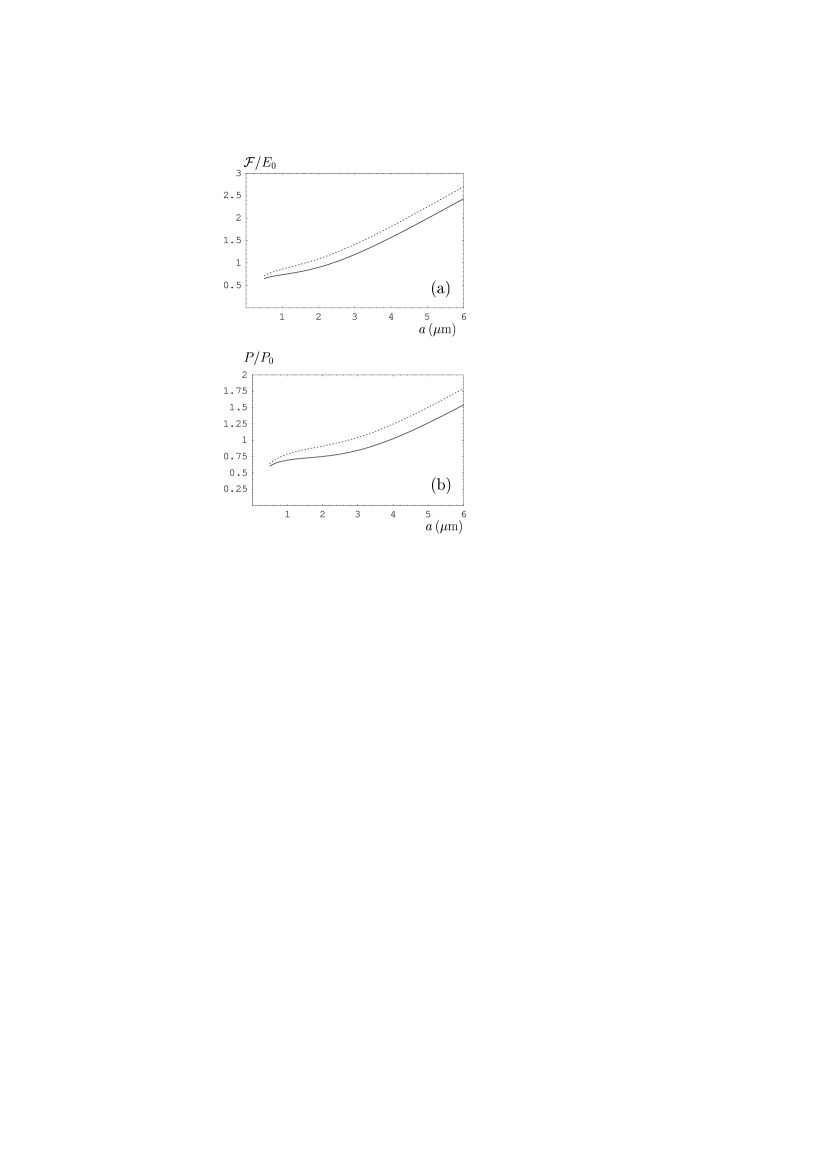
Figure 2: The relative Casimir free energy per unit area (a) and pressure (b) as functions of separation in the configuration of two parallel Co plates with account of magnetic properties (solid lines) and with magnetic properties disregarded (dashed lines). Computations are performed using the plasma model at $T=300\,$K.

Figure 3: The relative Casimir free energy per unit area (a) and pressure (b) as functions of separation in the configuration of two parallel Fe plates with account of magnetic properties (solid lines) and with magnetic properties disregarded (dashed lines). Computations are performed using the Drude model at $T=300\,$K.

Figure 4: The relative Casimir free energy per unit area (a) and pressure (b) as functions of separation in the configuration of two parallel Fe plates with account of magnetic properties (solid lines) and with magnetic properties disregarded (dashed lines). Computations are performed using the plasma model at $T=300\,$K.

Figure 5: The relative Casimir free energy per unit area (a) and pressure (b) as functions of separation in the configuration of one plate made of Co and the other plate made of Au. Computations are performed using the Drude model at $T=300\,$K.

Figure 6: The relative Casimir free energy per unit area (a) and pressure (b) as functions of separation in the configuration of one plate made of Co and the other plate made of Au with account of magnetic properties (solid lines) and with magnetic properties disregarded (dashed lines). Computations are performed using the plasma model at $T=300\,$K.

Figure 7: The relative Casimir free energy per unit area (a) and pressure (b) as functions of separation in the configuration of one plate made of Fe and the other plate made of Au. Computations are performed using the Drude model at $T=300\,$K.

Figure 8: The relative Casimir free energy per unit area (a) and pressure (b) as functions of separation in the configuration of one plate made of Fe and the other plate made of Au with account of magnetic properties (solid lines) and with magnetic properties disregarded (dashed lines). Computations are performed using the plasma model at $T=300\,$K.

Figure 9: The relative Casimir free energy per unit area (a) and pressure (b) as functions of separation at $T=300\,$K in the configuration of two parallel plates made of ferromagnetic dielectric with account of magnetic properties (solid lines) and with magnetic properties disregarded (dashed lines).

Figure 10: The relative Casimir free energy per unit area (a) and pressure (b) as functions of separation at $T=300\,$K in the configuration of one plate made of ferromagnetic dielectric and the other plate made of Au with account of magnetic properties (solid lines) and with magnetic properties disregarded (dashed lines). Computations are performed using the plasma model for Au.

Figure 11: The regions of the Casimir repulsion (above the solid line) and attraction (below the solid line) in the $[\varepsilon(0),\mu(0)]$-plane. See text for further discussion.

Figure 12: The static magnetic permeability of Gd in the magnetic phase transition as a function of temperature.

Figure 13: The relative Casimir free energy per unit area (a) and pressure (b) as functions of temperature in the configuration of two parallel Gd plates at the separation $a=0.5\,\mu$m. The solid and dashed lines take into account and disregard the magnetic properties, respectively. The pairs of lines marked 1 and 2 indicate the respective computational results obtained using the Drude and plasma models.

References

- (1) H. B. G. Casimir, Proc. K. Ned. Akad. Wet. 51, 793 (1948).
- (2) E. M. Lifshitz, Zh. Eksp. Teor. Fiz. 29, 94 (1956) [Sov. Phys. JETP 2, 73 (1956)].
- (3) I. E. Dzyaloshinskii, E. M. Lifshitz, and L. P. Pitaevskii, Usp. Fiz. Nauk 73, 381 (1961) [Adv. Phys. 38, 165 (1961)].
- (4) M. Kardar and R. Golestanian, Rev. Mod. Phys. 71, 1233 (1999).
- (5) M. Bordag, U. Mohideen, and V. M. Mostepanenko, Phys. Rep. 353, 1 (2001).
- (6) K. A. Milton, J. Phys. A: Math. Gen. 37, R209 (2004).
- (7) S. K. Lamoreaux, Rep. Progr. Phys. 68, 201 (2005).
- (8) P. W. Milonni, The Quantum Vacuum (Academic Press, San Diego, 1994).
- (9) M. Krech, The Casimir Effect in Critical Systems (World Scientific, Singapore, 1994).
- (10) V. M. Mostepanenko and N. N. Trunov, The Casimir Effect and its Applications (Clarendon, Oxford, 1997).
- (11) K. A. Milton, The Casimir Effect (World Scientific, Singapore, 2001).
- (12) S. K. Lamoreaux, Phys. Rev. Lett. 78, 5 (1997).
- (13) U. Mohideen and A. Roy, Phys. Rev. Lett. 81, 4549 (1998).
- (14) M. Bordag, G. L. Klimchitskaya, U. Mohideen, and V. M. Mostepanenko, Advances in the Casimir Effect (Oxford University Press, Oxford, 2009).
- (15) E. Buks and M. L. Roukes, Phys. Rev. B 63, 033402 (2001).
- (16) T. H. Boyer, Phys. Rev. 174, 1764 (1968).
- (17) T. H. Boyer, Phys. Rev. A 9, 2078 (1974).
- (18) F. C. Santos, A. Tenório, and A. C. Tort, Phys. Rev. D 60, 105022 (1999).
- (19) D. T. Alves, C. Farina, and A. C. Tort, Phys. Rev. A 61, 034102 (2001).
- (20) J. C. da Silva, A. Matos Neto, H. Q. Placido, M. Revzen, and A. E. Santana, Physica (Amsterdam) A 292, 411 (2001).
- (21) P. Richmond and B. W. Ninham, J. Phys. C: Solid St. Phys. 4, 1988 (1971).
- (22) S. Y. Buhmann, D.-G. Welsch, and T. Kampf, Phys. Rev. A 72, 032112 (2005).
- (23) M. S. Tomaš, Phys. Lett. A 342, 381 (2005).
- (24) Yu. S. Barash and V. L. Ginzburg, Usp. Fiz. Nauk 116, 5 (1975) [Sov. Phys. Usp. 18, 305 (1975)].
- (25) G. Feinberg and J. Sucher, Phys. Rev. A 2, 2395 (1970).
- (26) H. Safari, D.-G. Welsch, S. Y. Buhmann, and S. Scheel, Phys. Rev. A 78, 062901 (2008).
- (27) G. Bimonte, G. L. Klimchitskaya, and V. M. Mostepanenko, Phys. Rev. A 79, 042906 (2009).
- (28) O. Kenneth, I. Klich, A. Mann, and M. Revzen, Phys. Rev. Lett. 89, 033001 (2002).
- (29) D. Iannuzzi and F. Capasso, Phys. Rev. Lett. 91, 029101 (2003).
- (30) R. S. Decca, D. López, E. Fischbach, G. L. Klimchitskaya, D. E. Krause, and V. M. Mostepanenko, Phys. Rev. D 75, 077101 (2007).
- (31) R. S. Decca, D. López, E. Fischbach, G. L. Klimchitskaya, D. E. Krause, and V. M. Mostepanenko, Eur. Phys. J. C 51, 963 (2007).
- (32) W. J. Kim, M. Brown-Hayes, D. A. R. Dalvit, J. H. Brownell, and R. Onofrio, Phys. Rev. A 78, 020101(R) (2008).
- (33) R. S. Decca, E. Fischbach, G. L. Klimchitskaya, D. E. Krause, D. López, U. Mohideen, and V. M. Mostepanenko, Phys. Rev. A 79, 026101 (2009).
- (34) W. J. Kim, M. Brown-Hayes, D. A. R. Dalvit, J. H. Brownell, and R. Onofrio, Phys. Rev. A 79, 026102 (2009).
- (35) P. W. Selwood, Magnetochemistry (Interscience Publ., New York, 1956).
- (36) A. H. Morrish, The Physical Principles of Magnetism (J. Wiley, New York, 1965).
- (37) S. V. Vonsovskii, Magnetism (J. Wiley, New York, 1974).
- (38) M. Boström and B. E. Sernelius, Phys. Rev. Lett. 84, 4757 (2000).
- (39) C. Genet, A. Lambrecht, and S. Reynaud, Phys. Rev. A 62, 012110 (2000).
- (40) M. Bordag, B. Geyer, G. L. Klimchitskaya, and V. M. Mostepanenko, Phys. Rev. Lett. 85, 503 (2000).
- (41) S. J. Rahi, T. Emig, N. Graham, R. L. Jaffe, and M. Kardar, Phys. Rev. D 80, 085021 (2009).
- (42) B. W. Harris, F. Chen, and U. Mohideen, Phys. Rev. A 62, 052109 (2000).
- (43) F. Chen, U. Mohideen, G. L. Klimchitskaya, and V. M. Mostepanenko, Phys. Rev. A 74, 022103 (2006).
- (44) F. Chen, G. L. Klimchitskaya, V. M. Mostepanenko, and U. Mohideen, Phys. Rev. Lett. 97, 170402 (2006).
- (45) F. Chen, G. L. Klimchitskaya, V. M. Mostepanenko, and U. Mohideen, Phys. Rev. B 76, 035338 (2007).
- (46) R. S. Decca, E. Fischbach, G. L. Klimchitskaya, D. E. Krause, D. López, and V. M. Mostepanenko, Phys. Rev. D 68, 116003 (2003).
- (47) G. L. Klimchitskaya, U. Mohideen, and V. M. Mostepanenko, Rev. Mod. Phys. 81, 1827 (2009).
- (48) J. H. Van Vleck, The Theory of Electric and Magnetic Susceptibilities (Oxford University Press, Oxford, 1932).
- (49) C. M. Hurd, Contemp. Phys. 23, 480 (1982).
- (50) Magnetic Phase Transitions, ed. M. Ausloos (Springer, Berlin, 1983).
- (51) B. Barbara, D. Gignoux, and C. Vettier, Lectures on Modern Magnetism (Springer, Berlin, 1988).
- (52) A. Goldman, Handbook of Modern Ferromagnetic Materials (Springer, New York, 1999).
- (53) R. S. Turtelli, R. Grössinger, and C. Kussbach, J. Appl. Phys. 83, 1581 (1998).
- (54) D. K. Ghodgaonkar, V. V. Varadan, and V. K. Varadan, IEEE Trans. Instr. Meas. 39, 387 (1990).
- (55) I. Brevik, J. B. Aarseth, J. S. Høye, and K. A. Milton, Phys. Rev. E 71, 056101 (2005).
- (56) J. S. Høye, I. Brevik, J. B. Aarseth, and K. A. Milton, J. Phys. A: Math. Gen. 39, 6031 (2006).
- (57) V. B. Bezerra, R. S. Decca, E. Fischbach, G. L. Klimchitskaya, D. E. Krause, D. López, V. M. Mostepanenko, and C. Romero, Phys. Rev. E 73, 028101 (2006).
- (58) R. S. Decca, D. López, E. Fischbach, G. L. Klimchitskaya, D. E. Krause, and V. M. Mostepanenko, Ann. Phys. (N.Y.) 318, 37 (2005).
- (59) V. A. Parsegian, Van der Waals Forces: A Handbook for Biologists, Chemists, Engineers, and Physicists (Cambridge University Press, Cambridge, 2005).
- (60) M. A. Ordal, R. J. Bell, R. W. Alexander Jr., L. L. Long, and M. R. Querry, Appl. Otp. 24, 4493 (1985).
- (61) A. Lambrecht and S. Reynaud, Eur. Phys. J. D. 8, 309 (2000).
- (62) S. A. Chambers, Surf. Sci. Reports 61, 345 (2006).
- (63) R. K. Roy and A. N. Datta, J. Phys. D: Appl. Phys. 7, 1053 (1974).
- (64) R. R. Rakhimov, R. Bah, J. S. Hwang, S. P. Solodovnikov, I. A. Alexandrov, A. Yu. Karmilov, V. G. Shevchenko, E. S. Obolonkova, and A. I. Aleksandrov, J. Appl. Phys. 101, 09N504 (2007).
- (65) K. Kikoin, J. Magn. Magnetic Mat. 321, 702 (2008).
- (66) I. Tsukobara, J. Phys. Soc. Jpn. 15, 1664 (1960).
- (67) A. J. Behan, A. Mokhtari, H. J. Blythe, D. Score, X.-H. Xu, J. R. Neal, A. M. Fox, and G. A. Gehring, Phys. Rev. Lett. 100, 047206 (2008).
- (68) A. Tiwari, V. M. Bhosle, S. Ramachandran, N. Sudhakar, J. Narayan, S. Budak, and A. Gupta, Appl. Phys. Lett. 88, 142511 (2006).
- (69) V. A. Parsegian and G. H. Weiss, J. Coll. Interface Sci. 81, 285 (1981).
- (70) L. Lewin, J. Inst. Elect. Eng. (part C) 94, 64 (1947).
- (71) D. H. Martin, Magnetism in Solids (MIT Press, Cambridge, 1967).
- (72) H. E. Nigh, S. Legvold, and F. H. Spedding, Phys. Rev. 132, 1092 (1963).
- (73) F. Milstein and G. Zyvoloski, J. Appl. Phys. 43, 4217 (1972).
- (74) I. Coroiu, E. Culea, I. V. Simiti, and A. Darabont, J. Optoelectr. Adv. Mat. 8, 526 (2006).
- (75) J. M. D. Coey, V. Skumryev, and K. Gallagher, Nature 401, 35 (1999).
- (76) Handbook of Optical Constants of Solids III, ed. E. D. Palik (Academic, New York, 1998).
- (77) R. S. Decca, D. López, H. B. Chan, E. Fischbach, D. E. Krause, and C. R. Jamell, Phys. Rev. Lett. 94, 240401 (2005).
- (78) R. Castillo-Garza, C.-C. Chang, D. Jimenez, G. L. Klimchitskaya, V. M. Mostepanenko, and U. Mohideen, Phys. Rev. A 75, 062114 (2007).