We compute ${\cal N}=4$ Super Yang Mills planar amplitudes at strong coupling by considering minimal surfaces in $AdS_{5}$ space. The surfaces end on a null polygonal contour at the boundary of $AdS$. We show how to compute the area of the surfaces as a function of the conformal cross ratios characterizing the polygon at the boundary. We reduce the problem to a simple set of functional equations for the cross ratios as functions of the spectral parameter. These equations have the form of Thermodynamic Bethe Ansatz equations. The area is the free energy of the TBA system. We consider any number of gluons and in any kinematic configuration.

1 Introduction

In this paper we consider minimal area surfaces in $AdS$ space that end on a null polygonal contour at the boundary of $AdS$. Our goal is to compute the area of the surfaces as a function of the shape of the contour. Our solution to the problem consists of a system of integral equations of the thermodynamic Bethe ansatz (TBA) form [1]. The area is given by the TBA free energy of the system.

Our motivation for this investigation is the study of scattering amplitudes in ${\cal N}=4$ super Yang Mills. Planar ${\cal N}=4$ Super Yang Mills is an integrable theory [2]. This means that if one finds the appropriate trick, one is going to be able to perform computations for all values of the ’t Hooft coupling $\lambda$ [3, 4]. Finding the appropriate trick is usually tricky. Via the $AdS/CFT$ correspondence, this problem amounts to solving the quantum sigma model describing strings in $AdS_{5}\times S^{5}$. The classical limit of this theory is simpler to analyze. This is what we do in this paper. We consider classical solutions for strings moving in $AdS_{5}$. In the classical limit we can forget about the worldsheet fermions and the five sphere and study strings that are in $AdS_{5}$. We think that the knowledge of these classical solutions will be useful for solving the full quantum problem. Classical solutions that were useful for the problem of operator dimensions were considered in [5, 6] and several other papers. Here we consider classical solutions relevant for scattering amplitudes or Wilson loops.

A scattering amplitude at strong coupling corresponds to a surface that ends on the $AdS$ boundary on a very peculiar polygonal contour [7]. When we consider a color ordered amplitude involving $n$ particles with null momenta ${\bf k}_{1},\cdots,{\bf k}_{n}$ we get the following contour. The contour is specified by its ordered vertices ${\bf x}_{1},\cdots,{\bf x}_{n}$, with $x^{\mu}_{i}-x^{\mu}_{i-1}=k_{i}^{\mu}$, see figure 1. The problem becomes identical to the problem of computing a Wilson loop with this contour. In fact, we have a “dual conformal symmetry” which acts as the ordinary conformal symmetry on the positions ${\bf x}_{i}$ [8]. The amplitude has a divergent part and a finite part. The divergent part has a structure that is well understood [9]. In addition, a piece of the finite part is also known [9, 10]. There is an interesting finite piece which has not yet been computed in general. Two loop perturbative computations of this piece include [11, 12, 13, 14], and several subsequent papers. The interesting part of the amplitude is a function of conformal cross ratios of the ${\bf x}_{i}$. If we have $n$ points we have $3(n-5)$ independent cross ratios. At strong ’t Hooft coupling we can compute this in terms of the area of the minimal surface that ends on the polygonal contour [7].

Our method will use integrability of the sigma model in the following way. First we define a family of flat connections with a spectral parameter $\theta$. Sections of this flat connection can be used to define solutions which depend on the spectral parameter $\theta$. With these, we define a set cross ratios $Y_{k}(\theta)$. We find a functional $Y$ system that constrains the $\theta$ dependence of the functions $Y_{k}$. This system has $3(n-5)$ “integration constants" which come in when we specify the boundary conditions for $\theta\to\pm\infty$. We can restate these functional equations in terms of integral equations, where the $3(n-5)$ parameters appear explicitly. These integral equations have a TBA form. Schematically they are

$$\log Y_{k}(\theta)=-m_{k}\cosh\theta+c_{k}+K_{k,s}\star\log(1+Y_{s})$$

where the $m_{k}$ and $c_{k}$ are the $3(n-5)$ parameters we mentioned above and $K_{r,s}$ are some kernels. Moreover, the area has an expression in terms of the TBA free energy of the system.

$${\rm Area}=\int{d\theta\over 2\pi}m_{k}\cosh\theta\log(1+Y_{k}(\theta))$$

Evaluating $Y_{k}$ at $\theta=0$ we get the physical values of the cross ratios. However, we can view other values of $\theta$ as a one parameter family of cross ratios which give the same value for the area. Thus, changing $\theta$ generates a symmetry of the problem.

The case involving a six sided polygon was treated in [15] and the octagon, in a particular kinematic subspace, was considered in [16, 17]. Using this method, the area is computed without finding the explicit shape of the minimal surface.

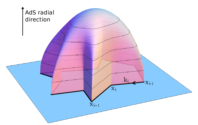
Figure 1: The polygon is specified at the $AdS$ boundary by the positions of the cusps ${\bf x}_{i}$. These positions are related to an ordered sequence of momenta ${\bf k}_{i}$ by ${\bf k}_{i}={\bf x}_{i}-{\bf x}_{i-1}$. The two dimensional minimal surface streches in the $AdS$ bulk and ends on the polygonal contour at the boundary.

Our paper is organized as follows. In section two we recall the connection between sigma models which obey the Virasoro constraints and Hitchin equations. In section three we discuss the case where the minimal surfaces are embedded in $AdS_{3}$. This is a warm up problem, which is simpler than the general problem. In section four we solve the full $AdS_{5}$ problem. We derive the $Y$ system, the integral equations and the area. We perform some checks. We also compute the exact answer for a one parameter family of regular polygons. Finally, we present some conclusions. We also have several appendices with useful details.

2 The classical sigma model and Hitchin equations

The classical $AdS_{5}$ sigma model is integrable. This can be shown by exhibiting a one parameter family of flat connections. For our problem, it will be convenient to choose this one parameter family in a special way which will simplify its asymptotic behavior on the worldsheet. In fact, to make this choice we will make use of the Virasoro constraints of the theory. This has been explained in detail in previous papers [18, 19, 20, 21, 22, 24]. Instead of repeating the whole discussion, we will present a slightly more abstract and algebraic version here.

2.1 General integrable theories and Hitchin equations

Let us assume that we have a coset space $G/H$. Let us assume that the Lie algebra $\mathcal{G}$ has a $Z_{2}$ symmetry that ensures integrability. In other words, imagine that the Lie algebra has the decomposition $\mathcal{G}=\mathcal{H}+\mathcal{K}$ so that $\mathcal{H}$ is left invariant under the action of the $Z_{2}$ generator while elements in $\mathcal{K}$ are sent to minus themselves. We then write the $G$ invariant currents $J=g^{-1}dg$. This is a flat current $dJ+J\wedge J=0$. We can decompose $J$ in terms its components along $\mathcal{H}$ and $\mathcal{K}$ as

$$J=g^{-1}dg=H+K$$ (1)

When we gauge the sigma model we add a gauge field along $\mathcal{H}$, and we can do local $H$ gauge transformations. The equations of motion of the system can be written in terms of the $H$-gauge invariant currents $k=gKg^{-1}$ as $d*k=0$. Notice that $k$ are the Noether currents of the problem. These equations of motion together with the flatness condition for $J$ lead to

$$D_{z}K_{\bar{z}}=0=D_{\bar{z}}K_{z}\leavevmode\nobreak\ ,\leavevmode\nobreak\ \leavevmode\nobreak\ \leavevmode\nobreak\ \leavevmode\nobreak\ \leavevmode\nobreak\ \leavevmode\nobreak\ \leavevmode\nobreak\ \leavevmode\nobreak\ \leavevmode\nobreak\ \leavevmode\nobreak\ \leavevmode\nobreak\ \leavevmode\nobreak\ [D_{z},D_{\bar{z}}]+[K_{z},K_{\bar{z}}]=0$$ (2)

$${\rm where}\leavevmode\nobreak\ \leavevmode\nobreak\ \leavevmode\nobreak\ \leavevmode\nobreak\ \leavevmode\nobreak\ D_{z}X\equiv\partial_{z}X+[H_{z},X]$$ (3)

We can view these as equations for the connection. Once we solve these, we can find a coset representative by solving the flatness condition

$$(d+J)g^{-1}=(d+H+K)g^{-1}=0$$ (4)

More precisely, we start with a set of independent vector solutions to the equation $(d+J)\psi=0$, orthonormalize them, and assemble them into $g^{-1}$. These vector solutions are called flat sections. The global $G$-symmetry acts by left multiplication of $g$ and the equations (2) are $G$ invariant. The equations (2) are identical to Hitchin’s equations after the identification $\hat{\Phi}_{z}=K_{z}$, $\hat{\Phi}_{\bar{z}}=K_{\bar{z}}$, $A=H$ . These equations are equivalent to the flatness of the one parameter family of connections

$$d+\hat{\cal A}(\zeta)\leavevmode\nobreak\ ,\leavevmode\nobreak\ \leavevmode\nobreak\ \leavevmode\nobreak\ \leavevmode\nobreak\ \leavevmode\nobreak\ \leavevmode\nobreak\ \leavevmode\nobreak\ \leavevmode\nobreak\ {\rm with}\leavevmode\nobreak\ \leavevmode\nobreak\ \leavevmode\nobreak\ \hat{\cal A}(\zeta)={K_{z}dz\over\zeta^{2}}+H+{\zeta^{2}\,K_{\bar{z}}d\bar{z}}$$ (5)

Flat sections of this connection, at $\zeta=1$, give back the group element $g^{-1}$. This connection differs from the connection that is often written (e.g. in [5]) by a gauge transformation by the group element $g$. Though we will not need it here, let us quote the more usual form of the flat connection

$$d+a\leavevmode\nobreak\ ,\leavevmode\nobreak\ \leavevmode\nobreak\ \leavevmode\nobreak\ \leavevmode\nobreak\ \leavevmode\nobreak\ \leavevmode\nobreak\ \leavevmode\nobreak\ {\rm with}\leavevmode\nobreak\ \leavevmode\nobreak\ \leavevmode\nobreak\ \leavevmode\nobreak\ \leavevmode\nobreak\ \leavevmode\nobreak\ \leavevmode\nobreak\ \leavevmode\nobreak\ a=g\hat{\cal A}g^{-1}-dgg^{-1}=k_{z}dz({1\over\zeta^{2}}-1)+k_{\bar{z}}d\bar{z}(\zeta^{2}-1)$$

We did not find this form of the flat connection particularly useful for our purposes.

The equations (2) imply that $T(z)={\rm Tr}[K_{z}^{2}]$ is holomorphic. This is the usual holomorphicity of the stress tensor. For the $SO(n+1)/SO(n)$ type cosets that we are interested in, higher traces of $K_{z}$ vanish, so we do not obtain any other interesting holomorphic quantities. In particular, if we are considering a theory obeying the Virasoro constraints, $T=0$, then we do not appear to get any interesting holomorphic quantities in this fashion.

2.2 Integrable theories with Virasoro constraints and Hitchin’s equations

As we mentioned above, in the case that $T=0$, we must work a bit harder in order to obtain interesting holomorphic quantities. In fact, it is possible to choose a slightly different form (or different gauge) for the connection so that we obtain a more interesting Hitchin system. This is a small variant of the Pohlmeyer type reduction. For the case with non-zero stress tensor this was described in [18, 21, 22]. In the particular case that is going to be of interest to us, which is the SO(2,4)/SO(1,5) or $AdS_{5}$ sigma model this was done in [19, 24, 15]. Since we do not want to repeat those derivations here, let us give a more abstract perspective on it.

We consider cosets of the form $G/H=SO(n+1)/SO(n)$, or $SO(2,n)/SO(1,n)$. Probably, similar considerations are true for other cosets but we have not checked the details. We now have the Virasoro constraints ${\rm Tr}[K_{z}^{2}]=0$ and ${\rm Tr}[K_{\bar{z}}^{2}]=0$. We assume that ${\rm Tr}[K_{z}K_{\bar{z}}]$ is generically non-zero. This quantity is the action density or the area element, so it will be non-zero for our solutions. We can then think of $K_{z}$ and $K_{\bar{z}}$ as spanning a two dimensional subspace of ${\mathcal{K}}$. We consider a generator $q$ in ${\mathcal{H}}$ such that $K_{z}$ has charge +1 and $K_{\bar{z}}$ has charge -1 under $q$. In other words, we view $K_{z}$ and $K_{\bar{z}}$ as two lightcone directions in the Lie algebra, and $q$ is the “boost" generator. We can further split the lie algebra ${\mathcal{H}}$ according to the charges under $q$. In our case, we have $\mathcal{H}^{(0)}$, $\mathcal{H}^{(1)}$ and $\mathcal{H}^{(-1)}$, where the superscript indicates the charge under $q$. We then take (5) and make a global gauge transformation by $\zeta^{q}$. We obtain

$${\cal A}=\zeta^{q}\hat{\cal A}\zeta^{-q}={1\over\zeta}(K_{z}+H^{(-1)}_{z})dz+H_{0}+\zeta(K_{\bar{z}}+H^{(1)}_{\bar{z}})d\bar{z}\equiv{\Phi_{z}dz\over\zeta}+A+\zeta\,\Phi_{\bar{z}}d\bar{z}$$ (6)

This is the final form of the flat connection that we will use. We saw that it is a simple transformation of the previous one. Moreover, when $\zeta=1$ the gauge transformation is trivial and the flat sections of this connection are still giving us the solution $g^{-1}$, as in (4). One nice aspect is that now $P(z)\equiv{1\over 4}Tr[\Phi_{z}^{4}]$ is a non-vanishing holomorphic current. One can wonder why we have a spin four holomorphic current. In general, the integrable theory has higher spin conserved currents. These higher spin currents are usually not holomorphic. When the stress tensor vanishes, the spin four current becomes holomorphic. In terms of embedding coordinates with $X^{2}=-1$, we have $P\propto\partial^{2}X\cdot\partial^{2}X$. We also have that $Tr[\Phi_{z}^{r}]=0$ for $r<4$. Finally, note that if we start from a general $SO(n)$ Hitchin equation, we can specialize into (6) by performing a $Z_{4}$ projection generated by the product of the $Z_{2}$ transformation we had above times a conjugation by $(i)^{q}$, where $q$ is the $U(1)$ generator we discussed above. This combined generator, let us call it $r$, should then give $r(\Phi_{z})=-i\Phi_{z}$, $r(\Phi_{\bar{z}})=i\Phi_{\bar{z}}$, $r(A)=A$. In section 4.1 we give a more explicit form for this generator.

In our case, we will further use the relation between $SO(2,4)$ and $SU(2,2)$ in order to write an $SU(2,2)$ flat connection. If we denote by $\psi$ the flat sections of the $SU(2,2)$ connection, then anti-symmetric products of two different sections $\psi$ and $\psi^{\prime}$ will give a flat section in the vector representation of $SO(2,4)$. Schematically $q^{A}=(\Gamma^{A})^{\alpha\beta}\psi_{[\alpha}\psi^{\prime}_{\beta]}$, where $\psi$ and $\psi^{\prime}$ are two solutions of the problem in the spinor (or fundamental of $SU(2,2)$) and $q^{A}$ is a solution in the vector representation of $SO(2,4)$.

Note that the action for the problem, which is equal to the area, is given by

$$A = \int d^{2}zTr_{SO(2,4)}[K_{z}K_{\bar{z}}]=2\int d^{2}zTr_{SU(2,2)}[K_{z}K_{\bar{z}}]$$

$$A = \int d^{2}zTr[\Phi_{z}\Phi_{\bar{z}}]+{\rm total\leavevmode\nobreak\ derivative}$$ (7)

The total derivative term is a constant proportional to the degree of the polynomial $P$ (and independent of the kinematics). In order to show the last equality in (7) we can take the trace of the generator $q$ times the second equation in (2) and use the Jacobi identity. (Alternatively, one can show it via an explicit parameterization as in [15].)

Once we compute this geometric area we can compute the amplitude, or the Wilson loop expectation value as

$${\rm Amplitude}\sim\langle W\rangle\sim e^{-{R^{2}\over 2\pi\alpha^{\prime}}A}=e^{-{\sqrt{\lambda}\over 2\pi}A}$$

Here $A$ is the geometrical area of the surface in units where the radius of AdS has been set to one. This area is infinite, but it can be regularized in a well understood fashion. The central object of this paper is certain regularized area, defined by

$$A_{reg}=\int d^{2}z\left(Tr[\Phi_{z}\Phi_{\bar{z}}]-4(P\bar{P})^{1/4}\right)$$ (8)

namely, we subtract the behavior of $Tr[\Phi_{z}\Phi_{\bar{z}}]$ far away. Since (8) is invariant under conformal transformations, it is a function of the cross-ratios. When using a physical regulator, the area will have additional terms. These additional terms are well understood and described in appendix G.

2.3 Flat sections, Stokes sectors and cross ratios

In this subsection we recall some facts, which were discussed in more detail in [15]. For the amplitude problem the worldsheet is the whole complex plane and $P(z)$ is a polynomial. We then study the problem $(d+{\cal A}(\zeta))\psi=0$. As we go to large $z$ some flat sections $\psi$ will diverge and some will go to zero. The fact that some diverge means that the worldsheet goes to the boundary of $AdS$ space. For large $z$, the boundary conditions are such that we can simultaneously diagonalize $\Phi(z)\sim P(z)^{1/4}{\rm diag}(1,-i,-1,i)$ and $\Phi_{\bar{z}}\sim\bar{P}^{1/4}(\bar{z}){\rm diag}(1,i,-1,-i)$. The particular relation between eigenvalues is determined by the $Z_{4}$ symmetry of the problem. This determines the large $z$ asymptotics of the four solutions

$$\psi_{a}\sim\exp\left\{-i^{-a}{\int P^{1/4}(z)dz\over\zeta}-i^{a}\zeta\int P^{1/4}(\bar{z})d\bar{z}\right\}\leavevmode\nobreak\ ,\leavevmode\nobreak\ \leavevmode\nobreak\ \leavevmode\nobreak\ \leavevmode\nobreak\ \leavevmode\nobreak\ \leavevmode\nobreak\ \leavevmode\nobreak\ a=0,1,2,3$$

The problem displays the Stokes phenomenon at large $z$. This means that the previous behavior of solutions is only valid within a given Stokes sector. The number of Stokes sectors is determined by the degree of the polynomial. Namely, for large $z$ we have $\int^{z}dz^{\prime}P(z^{\prime})^{1/4}\sim z^{n/4}+\cdots$, for a polynomial of degree $n-4$. In order to characterize the problem it is convenient to choose the smallest solution $s_{i}$ in each of the Stokes sectors. This smallest solution is well defined up to an overall rescaling. Given any four flat sections, it is possible to construct a gauge invariant inner product $\langle\psi_{1},\psi_{2},\psi_{3},\psi_{4}\rangle\equiv\epsilon^{\alpha\beta\gamma\delta}\psi_{1\alpha}\psi_{2\alpha}\psi_{3\gamma}\psi_{4\delta}$. This inner product is independent of the position where we compute it. A full solution of the problem is given by choosing four arbitrary flat sections $\psi_{1},\cdots\psi_{4}$ where the subindex runs over the four solutions, but each of them is a four component spinor. We will use greek letters for spinor components and latin letters for labeling different solutions. The target space conformal group $SU(2,2)$ acts on the latin indices, but not on the greek indices where the flat connection acts. The spacetime embedding coordinates $X^{I}$ are given in terms of these solutions at $\zeta=1$. More explicitly, $X^{I}\Gamma^{I}_{ab}=M^{\alpha\beta}\psi_{a\alpha}\psi_{b\beta,}$ where $M$ is a fixed matrix and $a,b$ are spacetime indices. As we go to large $z$, some of the solutions diverge. The particular combination of solutions that form the two solutions that diverge most rapidly, determines a ray $X^{I}$. This maps to a point on the boundary of $AdS_{5}$ space. We can find this point in a convenient way by picking the two smallest solutions which will be $s_{i}$ and $s_{i+1}$, if we are between Stokes sectors $i$ and $i+1$. Then the spacetime direction is obtained by taking

$$X^{i}_{ab}\propto\langle\psi_{a},\psi_{b},s_{i},s_{i+1}\rangle$$ (9)

This determines the direction in which $X^{i}_{ab}$ is diverging. Recall that we can think of the boundary of $AdS$ as a projective space, given by six coordinates $\hat{X}^{I}$, with $\hat{X}^{2}=0$ and $\hat{X}^{I}\sim\lambda\hat{X}^{I}$. Thus the diverging solution determines a point $\hat{X}$ in projective space, which is the same as saying that it determines a point on the boundary of $AdS$.

The index $i$ labels the cusp number. We can form quantities of the form $X^{i}\cdot X^{j}\propto\langle s_{i},s_{i+1},s_{j},s_{j+1}\rangle$. Finally, cross ratios are given by quantities of the form

$$Y_{ijkl}={X^{i}\cdot X^{j}\,X^{k}\cdot X^{l}\over X^{i}\cdot X^{k}\,X^{l}\cdot X^{j}}={\langle s_{i},s_{i+1},s_{j},s_{j+1}\rangle\langle s_{k},s_{k+1},s_{l},s_{l+1}\rangle\over\langle s_{i},s_{i+1},s_{k},s_{k+1}\rangle\langle s_{l},s_{l+1},s_{j},s_{j+1}\rangle}$$ (10)

The cross ratios do not depend on the normalization of each of the $s_{i}$.

These cross ratios are functions of the spectral parameter $\zeta$. In what follows, we will choose a convenient basis of cross ratios and study their $\zeta$ dependence. We will write an integral equation determining the values of the cross ratios as a function of $\zeta$. Finally we will express the area in terms of certain integrals of the cross ratios over $\zeta$.

3 Minimal surfaces in $AdS_{3}$

We first consider minimal surfaces that can be embedded in an $AdS_{3}$ subspace of $AdS_{5}$. This is a simpler problem that illustrates the method that we will use in the $AdS_{5}$ case. The reader that is only interested in the $AdS_{5}$ case can jump directly to the next section.

3.1 $AdS_{3}$ preliminaries

When the surface can be embedded in $AdS_{3}$ the problem simplifies and it reduces to a $Z_{2}$ projection of an $SU(2)$ Hitchin problem. The derivation of this fact is rather similar to what we discussed above and was treated in detail in [17]. We will not repeat the derivation, but we will state the final results. We have a polynomial $p=\frac{1}{2}Tr[\tilde{\Phi}_{z}^{2}]$ whose degree determines the number of cusps. We now have $SU(2)$ quantities $\tilde{\Phi}_{z},\leavevmode\nobreak\ \tilde{A},\tilde{\Phi}_{\bar{z}}$ which are in the adjoint of $SU(2)$ and we have the $Z_{2}$ projection condition $\tilde{\Phi}_{z}=-U\tilde{\Phi}_{z}U^{-1}$, $\tilde{\Phi}_{\bar{z}}=-U\tilde{\Phi}_{\bar{z}}U^{-1}$ and $\tilde{A}=U\tilde{A}U^{-1}$ where $U=\sigma_{3}$ is the usual Pauli matrix. This restricts the components of $\tilde{A}$ and $\tilde{\Phi}$ that are non-zero. General SU(2) Hitchin problems were studied in [25] and we are now considering a special case of their discussion, though we will rederive some of their formulas in a different way. We study sections of the flat connection which obey

$$(d+{\tilde{\Phi}_{z}dz\over\zeta}+\tilde{A}+\tilde{\Phi}_{\bar{z}}d\bar{z}\,\zeta)\psi(\zeta)=0$$

The $Z_{2}$ symmetry relates solutions $\psi(\zeta)$ with different values of the spectral parameter. Namely, if $\psi(\zeta)$ is a flat section with spectral parameter $\zeta$, then $\eta(\zeta)\equiv U\psi(e^{i\pi}\zeta)$ is a solution of the problem with spectral parameter $\zeta$. We can track how the small solutions change as we change $\zeta$ by looking at them in the large $z$ region. In a given Stokes sector the small solution contains a factor behaving as $e^{-\int^{z}\sqrt{p}dz^{\prime}\over\zeta}\sim e^{-z^{n/4}\over\zeta}$, where $n$ is determined by the degree of the polynomial and is equal to the number of cusps of the polygon. $n$ is even. There are $n/2$ Stokes sectors and thus $n/2$ small solutions $s_{i}$. As we change the phase of $\zeta$, the ray in the $z$ plane where this solution is smallest rotates accordingly. In particular, if we start with the solution $s_{i}(\zeta)$, which is the small in the $i$th Stokes sector, we find that $s_{i}(e^{2\pi i}\zeta)\propto s_{i+2}(\zeta)$ and $Us_{i}(e^{i\pi}\zeta)\propto s_{i+1}(\zeta)$. Note that the solutions do not come back to themselves after a shift by $e^{2\pi i}\zeta$. We can choose a solution $s_{1}$ in the first Stokes sector and define all others as $s_{j}=U^{j-1}s_{1}(e^{ji\pi}\zeta)$. Then, as we go around we have that $s_{{n\over 2}+1}=A(\zeta)s_{1}$. $A(\zeta)$ can be set to one when $n/2$ is odd. When $n/2$ is even it has a simple form that we will discuss later.

The full connection with spectral parameter is an $SL(2)$ connection and thus we can form an $SL(2)$ invariant product $\langle\psi\psi^{\prime}\rangle$ with two solutions. Now we have that

$$\langle s_{i},s_{j}\rangle(e^{i\pi}\zeta)=\langle s_{i+1},s_{j+1}\rangle(\zeta)$$ (11)

We can normalize $s_{1}$ so that $\langle s_{1},s_{2}\rangle=1$. Then (11) also implies that $\langle s_{i},s_{i+1}\rangle=1$.

Figure 2: Spacetime positions of the cusps for a polygon that is embedded in $R^{1,1}$, which is the boundary of $AdS_{3}$. The positions of the cusps are given by a set of $n/2$ values $x^{+}_{i}$ and a set of $n/2$ values $x^{-}_{i}$.

We can form cross ratios by forming quantities like

$$\chi_{ijkl}(\zeta) = {\langle s_{i},s_{j}\rangle\langle s_{k},s_{l}\rangle\over\langle s_{i},s_{k}\rangle\langle s_{j},s_{l}\rangle}$$ (12)

These quantities do not depend on the arbitrary normalization of the $s_{i}$. By construction they are also invariant under the conformal symmetries of $AdS_{3}$. They can be related to the conformal invariant cross ratios formed from the positions of the cusps of the polygon. Recall that a polygon in $AdS_{3}$ is given by $n/2$ positions $x_{i}^{+}$ and $n/2$ positions $x^{-}_{i}$, see figure 2. We can form spacetime cross ratios from the positions of the points $x_{i}^{\pm}$. These spacetime cross ratios can be expressed in terms of the cross ratios in (12) as

$$\chi_{ijkl}(\zeta=1) = {x^{+}_{ij}x^{+}_{kl}\over x^{+}_{ik}x^{+}_{jl}}$$ (13)

$$\chi_{ijkl}(\zeta=i) = {x^{-}_{ij}x^{-}_{kl}\over x^{-}_{ik}x^{-}_{jl}}$$ (14)

3.2 The $AdS_{3}$ functional Y-system

We will now derive a set of functional equations for the inner products, or Wronskians, $\langle s_{i},s_{j}\rangle(\zeta)$ made out of two small solutions of the linear problem. The starting point is the Schouten identity, $\langle s_{i},s_{j}\rangle\langle s_{k},s_{l}\rangle+\langle s_{i},s_{l}\rangle\langle s_{j},s_{k}\rangle+\langle s_{i},s_{k}\rangle\langle s_{l},s_{j}\rangle=0$, applied to a particular choice of small solutions:

$$\langle s_{k+1},s_{-k}\rangle\langle s_{k},s_{-k-1}\rangle=\langle s_{k+1},s_{-k-1}\rangle\langle s_{k},s_{-k}\rangle+\langle s_{k},s_{k+1}\rangle\langle s_{-k-1},s_{-k}\rangle\,.$$ (15)

In our normalization the last two brackets are equal to one. Using (11) we see that this identity becomes the $SU(2)$ Hirota equation

$$T_{s}^{+}T_{s}^{-}=T_{s+1}T_{s-1}+1\,,$$ (16)

$${\rm where:}\leavevmode\nobreak\ \leavevmode\nobreak\ \leavevmode\nobreak\ \leavevmode\nobreak\ \leavevmode\nobreak\ \leavevmode\nobreak\ \leavevmode\nobreak\ T_{2k+1}=\langle s_{-k-1},s_{k+1}\rangle\leavevmode\nobreak\ ,\leavevmode\nobreak\ \leavevmode\nobreak\ \leavevmode\nobreak\ \leavevmode\nobreak\ \leavevmode\nobreak\ \leavevmode\nobreak\ \leavevmode\nobreak\ \leavevmode\nobreak\ \leavevmode\nobreak\ \leavevmode\nobreak\ T_{2k}=\langle s_{-k-1},s_{k}\rangle^{+}$$ (17)

or more uniformly $T_{s}=\langle s_{0},s_{s+1}\rangle(e^{-i(s+1)\pi/2}\zeta)$. The superscripts $\pm$ indicate a shift in spectral parameter, $f^{\pm}\equiv f(e^{\pm i{\pi\over 2}}\zeta)$. Actually, from (15) we get (16) for $s=2k$. For $s$ odd we need to start from a slightly different choice of indices in (15). $T_{s}$ is non-zero for $s=0,\dots,n/2-2$. Finally, we introduce the $Y$-functions $Y_{s}\equiv T_{s-1}T_{s+1}$. Being a product of two next-to-nearest-neighbor $T$-functions, the $Y$-functions are non-zero in a slightly smaller lattice parametrized by $s=1,\dots,n/2-3$. The number of $Y$-functions coincides with the number of independent cross ratios.

The Hirota equation (16) implies the Y-system for these new quantities:

$$Y_{s}^{+}Y_{s}^{-}=(1+Y_{s+1})(1+Y_{s-1})\,.$$ (18)

These equations are of course not enough to fix the Y-functions. After all they came from a trivial determinant identity without any information on the dynamics! To render them more restrictive we need to supplement them with the analytic properties of the Y-functions. This will then pick the appropriate solutions to these equations. Furthermore, to make these solutions useful we must relate them to the actual expression for the area. Before considering these points let us comment on some general properties of Hirota equations and their corresponding Y-systems.

3.3 Hirota equation, gauge invariance and normalization of small solutions

The general form of the Hirota system of equations – which generalizes the $SU(2)$ case derived above – is a set of functional equations for functions $T_{a,s}(\zeta)$. The indices $a,s$ take integers values and can be thought of as parametrizing a two dimensional lattice. At each point of this lattice we have a function $T_{a,s}(\zeta)$ of the spectral parameter $\zeta$. Then, for each site $o=(a,s)$ we have an Hirota equation

$$T_{o}^{+}T_{o}^{-}=T_{\leftarrow}T_{\rightarrow}+T_{\uparrow}T_{\downarrow}$$ (19)

involving the function at that site and the four $T$-functions at the four nearest-neighbor sites, $T_{\rightarrow}\equiv T_{a,s+1}$, $T_{\uparrow}=T_{a+1,s}$, etc. Recall that $T_{o}^{\pm}=T_{o}(e^{\pm i\pi/2}\zeta)$. This equation has a huge gauge redundancy

$$T_{a,s}\to\prod_{\alpha,\beta=\pm}g_{\alpha\beta}\left(e^{\frac{i\pi}{2}(\alpha a+\beta s)}\zeta\right)T_{a,s}(\zeta)$$

where $g_{\alpha\beta}(\zeta)$ are four arbitrary functions. It is therefore instructive to construct a set of gauge invariant quantities

$$Y_{o}=\frac{T_{\leftarrow}T_{\rightarrow}}{T_{\uparrow}T_{\downarrow}}\leavevmode\nobreak\ \leavevmode\nobreak\ \leavevmode\nobreak\ \leavevmode\nobreak\ \leavevmode\nobreak\ \leavevmode\nobreak\ \leavevmode\nobreak\ \leavevmode\nobreak\ \leavevmode\nobreak\ \leavevmode\nobreak\ \leavevmode\nobreak\ \leavevmode\nobreak\ {\rm or}\leavevmode\nobreak\ \leavevmode\nobreak\ \leavevmode\nobreak\ \leavevmode\nobreak\ \leavevmode\nobreak\ \leavevmode\nobreak\ \leavevmode\nobreak\ Y_{a,s}={T_{a,s-1}T_{a,s+1}\over T_{a+1,s}T_{a-1,s}}$$ (20)

It is instructive to think of the gauge invariant quantity $Y_{o}$ as a field strength made of the gauge dependent gauge field $T_{o}$. Suppose the $T$-functions are non-zero in some rectangular domain in the $(a,s)$ lattice. At the edges of the rectangle either the first or the second term in the right hand side of (19) is zero. We are left with a discrete Laplace equation for (the logarithm of) the $T$-functions and therefore they become pure gauge. At these boundary points the $Y$-functions are trivial (either zero or infinity) as expected from the analogy. The $Y$-functions are non-trivial in a smaller rectangle obtained from by removing the first and last columns and rows of the original domain.

The Hirota equation 19 then translates into the $Y$-system

$$\frac{Y_{o}^{+}Y_{o}^{-}}{Y_{\uparrow}Y_{\downarrow}}=\frac{(1+Y_{\leftarrow})(1+Y_{\rightarrow})}{(1+Y_{\uparrow})(1+Y_{\downarrow})}$$ (21)

for these gauge invariant quantities. Different domains in $a,s$ where $Y$’s are nontrivial together with different boundary condition and analytic properties describe different integrable models.

In the treatment of the previous section we considered the case where the $T$-functions live in a finite strip with three rows and $n/2-1$ columns, where $n$ is the number of gluons, see figure 3. The functions denoted by $T_{s}$ in that section are the T-functions in the non-trivial middle row, $T_{s}=T_{1,s}$. Similarly $Y_{s}=Y_{1,s}$. The $T$-functions introduced in that section are inner products of small solutions and are therefore sensitive to their normalization. This arbitrariness is a manifestation of the gauge freedom in Hirota equation. The normalization $\langle s_{i},s_{i+1}\rangle=1$ corresponds to the gauge choice where

$$\begin{array}[]{l}T_{0,2k}\equiv\langle s_{-k-1},s_{-k}\rangle\,,\\ T_{2,2k}\equiv\langle s_{k},s_{k+1}\rangle\,,\end{array}\leavevmode\nobreak\ \qquad\begin{array}[]{l}T_{0,2k+1}\equiv\langle s_{-k-2},s_{-k-1}\rangle^{+}\,,\\ T_{2,2k+1}\equiv\langle s_{k},s_{k+1}\rangle^{+}\,,\end{array}$$

are gauge fixed to one. We could of course opt not to fix a normalization for the T-functions but then we should use the gauge invariant combination (20) when defining the Y-functions:

$$Y_{2k} = \frac{T_{1,2k-1}T_{1,2k+1}}{T_{0,2k}T_{2,2k}}={\langle s_{-k},s_{k}\rangle\langle s_{-k-1},s_{k+1}\rangle\over\langle s_{-k-1},s_{-k}\rangle\langle s_{k},s_{k+1}\rangle}$$ (22)

$$Y_{2k+1} = \frac{T_{1,2k}T_{1,2k+2}}{T_{0,2k+1}T_{2,2k+1}}=\left[{\langle s_{-k-1},s_{k}\rangle\langle s_{-k-2},s_{k+1}\rangle\over\langle s_{-k-2},s_{-k-1}\rangle\langle s_{k},s_{k+1}\rangle}\right]^{+}\leavevmode\nobreak\ .$$

We see that they are now manifestly independent of the choice of the normalization of the small solutions. At spectral parameter $\zeta=1$, or $\zeta=e^{\pm i\pi/2}$ they yield physical space-time cross-ratios as in (13) (14).

A particularly interesting quantity is

$$B(\zeta)=\frac{Y_{n/2-3}}{Y_{n/2-5}}\ \frac{Y_{n/2-7}}{Y_{n/2-9}}\ \frac{Y_{n/2-11}}{Y_{n/2-13}}\ \dots\leavevmode\nobreak\$$ (23)

It follows from the $Y$-system equations (18) that $B^{+}B^{-}=1$. $B(\zeta)$ is constructed from the $Y$-functions and is therefore gauge invariant. Using the definition of the $Y$-functions we see that $B(\zeta)$ is given by a bunch of boundary $T$-functions. In our normalization all these functions except for the rightmost one are gauged to one. We find therefore $B=T_{1,n/2-2}=\langle s_{1},s_{n/2}\rangle\left(e^{-i\pi(n/2+1)/2}\zeta\right)$. This means that $B(\zeta)$ is the function that governs the monodormy $s_{n/2}=-B(\zeta e^{i\pi(n/2+1)/2})s_{0}$ of the small solutions.

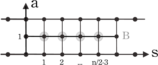
Figure 3: In this figure we have summarized the structure of the $T$’s and the $Y$’s in a gauge where we simplified the $T$’s that can be simplified. The small solid black dots represent non-zero $T$-functions. They are equal to one unless $a=1$ and $s=1,\dots,n/2-2$. At the rightmost point in this line we have $T_{1,n/2-2}=B$ where $B$ is a function which cannot be set to one only in the case that $n/2$ is even. In fact, in our case it is $B=-e^{m/\zeta+{\bar{m}}\zeta}$. This is the function that governs the monodormy $s_{n/2}=-B(\zeta e^{i\pi(n/2+1)/2})s_{0}$. The $Y$-functions are finite in the points indicated by fat gray shaded balls. At all other points they are either zero or infinity.

3.4 Analytic properties of the $Y$-functions

For finite values of $\zeta$ it is clear from (17) that the $T_{s}$ are analytic functions of $\zeta$, for $\zeta\not=0,\infty$. Generically, they will not be periodic under $\zeta\to e^{2\pi i}\zeta$. In general, the $Y$’s will be meromorphic functions. However, in our case, since we can choose to set the denominators to one, we see that the $Y$s have no poles and are thus analytic away from $\zeta=0,\infty$. For $\zeta\to 0$ and $\zeta\to\infty$ they will have essential singularities. In this section we analyze the behavior in these two regions.

When $\zeta\to 0$ we can solve the equations for the flat sections by making a WKB approximation, where $\zeta$ plays the role of $\hbar$. This is explained in great detail in [25], here we will summarize that discussion and apply it to our case. The final result is that, for an appropriate choice of the polynomial $p$, we have the standard boundary conditions in TBA equations. We will later discuss what happens for more general polynomials.

We are considering the equation

$$\left(d+{\Phi_{z}dz\over\zeta}+A+\zeta\,{\Phi_{\bar{z}}d\bar{z}}\right)s=0$$

When $\zeta\to 0$, it is convenient to make a similarity transformation that diagonalizes $\Phi_{z}\to\sqrt{p}\,{\rm diag}(1,-1)$. The solutions in this approximation go like $\exp\left(\pm\frac{1}{\zeta}\int\sqrt{p}dz\right)$ times constant vectors. The WKB is a good approximation if we are following the solution along a line of steepest descent. This is a line where the variation of the exponent, is real, ${\rm Im}(\sqrt{p(z)}\dot{z}/\zeta)=0$. This condition is an equation which determines the WKB lines. Through each point in the $z$ plane we have one such line going through. At the single zeros of $p$ we have three lines coming in. The WKB approximation fails at the zeros of $p$ (which are the turning points). From each Stokes sector we have WKB lines that emanate from it. These lines can end in other Stokes sectors or, for very special lines, on the zeros of $p$. If a line connects two Stokes sectors, say $i$ and $j$, then we can use it to approximate reliably the inner product $\langle s_{i},s_{j}\rangle$. This estimate is good in a sector of width $\pi$ in the phase of $\zeta$, centered on the value of $\zeta$ where the line exists. As we change the phase of $\zeta$ the pattern of flow lines changes. It also changes when we change the polynomial $p$. We first select a polynomial with all zeros along the real axis and such that $p(z)>0$ for large enough values of $z$ along the real line.

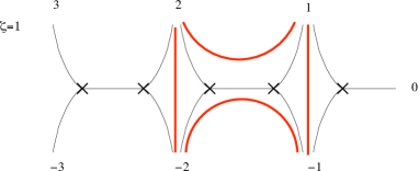
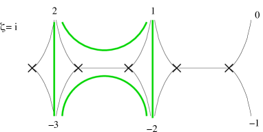
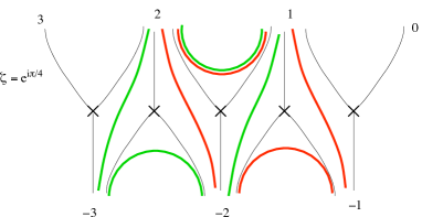
Figure 4: Sketch of the pattern of WKB lines for various phases of $\zeta$. The crosses denote the various zeros of $p(z)$. The numbers indicate the various Stokes sectors. The black thin lines end on the zeros and separate different classes of WKB lines. The thick colored lines are the WKB lines that we use to evaluate cross ratios. Here we have indicated only the ones used to evaluate $Y_{2}$ and $Y_{3}$. Finally, note that by setting the phase of $\zeta$ to $e^{i\pi/4}$ we have WKB lines that enable us to evaluate all the $Y_{s}$.

With this choice the pattern flows for WKB lines is shown in figure 4, for some values of the phase of $\zeta$. The WKB lines ending on zeros separate regions where lines flow between different Stokes sectors. In our problem we have some inner products evaluated at $\zeta$ and some and $i\zeta$. The flows for $\zeta=1$ and $\zeta=i$ are displayed on the top of figure 4, and they can be used to evaluate the various inner products. Alternatively, we can set $\zeta=e^{i\pi/4}$, evaluate them all and then continue them from this region. The resulting flow pattern is sketched on the bottom of figure 4.

Using those flow patterns it is a simple matter to evaluate various inner products. It turns out that the inner products in the definitions of the Y-functions (22) combine to give a contour integral around a certain cycles. See figure 5. Thus, each $Y_{s}$, is estimated by the integral of $\sqrt{p}$ along a cycle $\gamma_{s}$. We can call

$$Z_{s}=-\oint_{\gamma^{s}}\sqrt{p}dz$$

and the corresponding $Y$ functions have the small $\zeta$ behavior

$$\log Y_{2k}\sim{Z_{2k}\over\zeta}+\cdots\leavevmode\nobreak\ ,\leavevmode\nobreak\ \leavevmode\nobreak\ \leavevmode\nobreak\ \leavevmode\nobreak\ \leavevmode\nobreak\ \leavevmode\nobreak\ \leavevmode\nobreak\ \leavevmode\nobreak\ \leavevmode\nobreak\ \leavevmode\nobreak\ \leavevmode\nobreak\ \log Y_{2k+1}\sim{Z_{2k+1}\over i\zeta}+\cdots$$

In figure 5 we display the cycles corresponding to each of the $Y_{s}$.

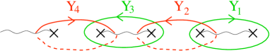
Figure 5: Cycles along which we need to integrate $\sqrt{p}dz$ in order to determine the asymptotic form of $Y_{s}$. By being careful about the sheet selected by the various small solutions one can determine the cycle orientations shown here.

It is convenient to define the parameters $m_{s}$ via

$$m_{2k}=-2Z_{2k}\leavevmode\nobreak\ \leavevmode\nobreak\ \leavevmode\nobreak\ \leavevmode\nobreak\ \leavevmode\nobreak\ \leavevmode\nobreak\ \leavevmode\nobreak\ \leavevmode\nobreak\ \leavevmode\nobreak\ \leavevmode\nobreak\ \leavevmode\nobreak\ \leavevmode\nobreak\ m_{2k-1}=-2Z_{2k+1}/i$$ (24)

For our choice of polynomial the $m_{s}$ are all real and positive. In order to check the positivity of the $m_{s}$ we need to be careful with the choice of branch when we evaluate the cross ratios. The two branches correspond to the two eigenvalues of $\Phi_{z}$ and differ by an overall sign. Taking the same cycles but on different branches is equivalent to changing the sign of $Z$. The correct branch is determined by the behavior of the various small solutions, each of which goes like $e^{\pm\int\sqrt{p}dz}$. After taking this into account we can check that the $m_{s}$ are indeed positive for the polynomial we chose.

A similar computation at large $\zeta$ gives a similar result, with $\log Y_{2k}\sim\zeta\bar{Z}_{2k}$. Thus, we have shown that all the $Y$ functions have the asymptotic behavior

$$\log Y_{s}=-m_{s}\cosh\theta+\cdots$$

for large $\theta$, $\zeta=e^{\theta}$.

Furthermore, this behavior is good over a range of $(-\pi,\pi)$ in the imaginary part of $\theta$. The reason is the following. For each $Y_{s}$, the region of $Im(\theta)=0$ corresponds to the center of the region where the WKB line exists. Furthermore, the corresponding WKB lines exist for a sector of angular size $\pi$ around this line. In addition, we have mentioned that the WKB approximation continues to be good for a further sector of $\pi/2$ on each side. In fact, this is more than enough for deriving the integral equations.

3.5 Integral form of the equations

The analytic properties derived above together with the functional equations (18) uniquely determine the $Y$-functions. However, for practical purposes – specially for numerics – it is useful to have an equivalent formulation of these $Y$-system equations in terms of TBA-like integral equations.

To derive them we follow the usual procedure which we briefly review for completeness. We note that $l_{s}\equiv\log(Y_{s}/e^{-m_{s}\cosh\theta})$ is analytic in the strip $|{\rm Im}(\theta)|\leq\pi/2$, vanishes as $\theta$ approaches infinity in this strip, and obeys

$$l_{s}^{+}+l_{s}^{-}=\log(1+Y_{s+1})(1+Y_{s-1})$$

which is nothing but the logarithm of the Y-system equations. Now we convolute this equation with the kernel

$$K(\theta)=\frac{1}{2\pi\cosh\theta}$$

to get

$$K\star(l_{s}^{+}+l_{s}^{-})\equiv\int\limits_{-\infty}^{+\infty}\frac{dy}{2\pi}\,\frac{l_{s}(y+i\pi/2)+l_{s}(y-i\pi/2)}{\cosh(x-y)}=\oint\limits_{\gamma}\frac{dy}{2\pi i}\,\frac{l_{s}(y)}{\sinh(x-y)}=l_{s}(x)$$

where $\gamma$ is the rectangle made out of the boundaries of the physical strip together with two vertical segments at ${\rm Re}(\theta)\to\pm\infty$. In order to be able to add these extra segments to the integral thus making it a contour integral, it was important to use the $l_{s}$ instead of $\log Y_{s}$. This is why this quantity was introduced in the first place. Furthermore, in the last step we used the fact that $l_{s}$ has no singularities inside the physical strip, this is an important input on the analytic properties of the $Y$-functions. Rewriting $l_{s}$ in terms of $Y_{s}$ leads therefore to the desired form of the integral equations:

$$\log Y_{s}=-m_{s}\cosh\theta+K\star\log(1+Y_{s+1})(1+Y_{s-1})\,.$$ (25)

For a given choice of masses $m_{s}$, the solution to these integral equations is unique and a basis of cross ratios can be read from evaluating the $Y_{s}(\theta)$’s at $\theta=0$. These equations are of the form of those appearing in the study of the TBA [1] for quantum integrable models in finite volume. Furthermore, as explained in the next section, the (regularized) area of the minimal surfaces turns out to be given in terms of the $Y$-functions as the free energy of the corresponding integrable model.

Up to now we have discussed the case where the zeros of the polynomial are along the real axis. Let us briefly discuss what happens as we start moving the zeros of the polynomial away from the real axis. Notice that the functional $Y$ system equations (18) do not depend on the polynomial. Thus, these equations continue to be true, regardless of its form. What changes are the asymptotic boundary conditions.

Let us consider first the case were we start from the above polynomial and we move the zeros around a little bit. Then the above derivation of the asymptotic form of the $Y$ functions goes through with only one change. Namely the quantities $Z_{s}$ and $m_{s}$ are now more general complex numbers and the asymptotic behavior is

$$\log Y_{s} \sim -{m_{s}\over 2\zeta}\leavevmode\nobreak\ ,\leavevmode\nobreak\ \leavevmode\nobreak\ \leavevmode\nobreak\ \leavevmode\nobreak\ \leavevmode\nobreak\ \leavevmode\nobreak\ \leavevmode\nobreak\ \leavevmode\nobreak\ {\rm for}\leavevmode\nobreak\ \leavevmode\nobreak\ \leavevmode\nobreak\ \leavevmode\nobreak\ \leavevmode\nobreak\ \leavevmode\nobreak\ \zeta\to 0$$

$$\log Y_{s} \sim -{\bar{m}_{s}\over 2}\zeta\leavevmode\nobreak\ ,\leavevmode\nobreak\ \leavevmode\nobreak\ \leavevmode\nobreak\ \leavevmode\nobreak\ \leavevmode\nobreak\ \leavevmode\nobreak\ \leavevmode\nobreak\ \leavevmode\nobreak\ {\rm for}\leavevmode\nobreak\ \leavevmode\nobreak\ \leavevmode\nobreak\ \leavevmode\nobreak\ \leavevmode\nobreak\ \leavevmode\nobreak\ \zeta\to\infty$$

In this case, when we derive the integral equation, it is convenient to shift the line where the $Y$ functions are integrated to be along the direction where $m_{s}/\zeta\equiv|m_{s}|e^{i\varphi_{s}}/\zeta$ is real and positive, which also makes $\bar{m}_{s}\zeta$ real and positive. Then, defining $\tilde{Y}_{s}(\theta)=Y_{s}(\theta+i\varphi_{s})$ we find that the integral equations have the form

$$\log\widetilde{Y}_{s}=-|m_{s}|\cosh\theta+K_{s,s+1}\star\log(1+\widetilde{Y}_{s+1})+K_{s,s-1}\star\log(1+\widetilde{Y}_{s-1})$$ (26)

where now $K_{s,s^{\prime}}=1/\cosh(\theta-\theta^{\prime}+i\varphi_{s}-i\varphi_{s^{\prime}})$.

As long as $|\varphi_{s}-\varphi_{s+1}|<\pi/2$, the integral equations conserve the form that we have derived. If we deform the phases beyond that regime we will have to change the form of the integral equations by picking the appropriate pole contributions from the kernels (which become singular for $|\varphi_{s}-\varphi_{s+1}|=\pi/2,3\pi/2,\dots$). Of course, the integral equation changes but the $Y$’s and therefore the area are continuous. The pattern under which the integral equation changes is explained in appendix B. This is the wall crossing phenomenon d iscussed in [26, 25].

These integral equations are a special case of the general case discussed in [26]. In fact, the equations in [26] are true for an arbitrary ${\cal N}=2$ theory, and a Hitchin problem is just a special case. Due to the $Z_{2}$ projection we have that the $\mathcal{X}_{\gamma}$ quantities in [26] obey the additional property $\mathcal{X}_{-\gamma}(\zeta)=\mathcal{X}_{\gamma}(-\zeta)$. Using this, we can easily map the kernel in [26] to the ${1\over\cosh}$ found here.

3.6 Area and free energy

As we mentioned above, the interesting part of the area is given by the integral

$$A=2\int d^{2}zTr[\tilde{\Phi}_{z}\tilde{\Phi}_{\bar{z}}]$$ (27)

By definition, the area is independent of $\zeta$.

It is convenient to think again about the small $\zeta$ regime and the WKB approximation that we did for small $\zeta$. In fact, we can improve on the WKB approximation and find the next couple of terms by systematically expanding the expressions for the inner products. We take complex masses but with small enough phases so that the WKB approximations that we did before continue to be valid, with the same cycles.. The final At this point it is convenient to use slightly different functions defined by

$$\widehat{Y}_{2k}(\zeta)=Y_{2k}(\zeta)\leavevmode\nobreak\ ,\leavevmode\nobreak\ \leavevmode\nobreak\ \leavevmode\nobreak\ \leavevmode\nobreak\ \leavevmode\nobreak\ \leavevmode\nobreak\ \leavevmode\nobreak\ \leavevmode\nobreak\ \widehat{Y}_{2k+1}=Y_{2k+1}^{-}=Y_{2k+1}(\zeta e^{-i\pi/2})$$ (28)

in order to undo the shifts in (22). With these definitions we find that

$$\log\widehat{Y}_{k}\ \sim -\left[{\oint_{\gamma_{k}}\lambda\over\zeta}+\oint_{\gamma_{k}}\alpha+\zeta\,\oint_{\gamma_{k}}u+\cdots\right]$$

$$\lambda=xdz\leavevmode\nobreak\ ,\leavevmode\nobreak\ \leavevmode\nobreak\ \leavevmode\nobreak\ \leavevmode\nobreak\ \leavevmode\nobreak\ \leavevmode\nobreak\ \leavevmode\nobreak\ \leavevmode\nobreak\ \leavevmode\nobreak\ x^{2}=p(z)$$

where $u$ is an exact one form. Here $\alpha$ given by the diagonal components of the connection $A$. In our case $\alpha=0$ due to the $Z_{2}$ projection. (But even if $\alpha$ were non-zero, it would not affect what we say below.) We know that $u$ is exact because we can deform the contour and $\log Y_{s}$ should not change. It has a $u_{z}$ and a $u_{\bar{z}}$ component. For our purposes, it will only be important to compute the $u_{\bar{z}}$ component which is

$$u^{i}_{\bar{z}}=\tilde{\Phi}^{ii}_{\bar{z}}$$ (30)

where the index $i$ is not summed over. In other words, we get the diagonal components of $\tilde{\Phi}_{\bar{z}}$ and we get the first or second diagonal component depending on whether we are on the first or second sheet of the Riemann surface. That is, $u$ is a one form on the Riemann surface, not on the $z$ plane. In the basis where $\tilde{\Phi}_{z}$ is diagonal, we can thus rewrite (27), using (30), as

$$A={i}\int\lambda\wedge u=-i\sum_{r,s}w_{rs}\oint_{\gamma^{r}}\lambda\oint_{\gamma^{s}}u$$

where ${\gamma^{r}}$ are a basis of cycles. We will take this basis to be the basis of cycles that gives the WKB approximation to the $Y_{s}$, see figure 5, and $w_{rs}$ is the inverse of the intersection form of the cycles. The matrix of cycle intersections can be read off from figure 5 and it is summarized in figure 6.

Figure 6: Intersection form $\theta^{r,s}$ for all the cycles associated to the $Y$ functions. This is computed from the cycles in figure 5. If an arrow points from $Y_{s}$ to $Y_{r}$, then we have $\langle\gamma_{s},\gamma_{r}\rangle=1$, otherwise the intersection vanishes.

We can also compute the small $\zeta$ behavior of $\widehat{Y}_{k}$ by expanding the integral equations (25). We get

$$\log\widehat{Y}_{r}=Z^{r}/\zeta+\zeta\left[\bar{Z}^{r}+\sum_{s}\theta^{rs}{1\over\pi i}\int{d\zeta^{\prime}\over\zeta^{\prime}}{1\over\zeta^{\prime}}\log(1+\widehat{Y}_{s})\right]$$ (31)

It turns out that $\theta^{rs}$ is given by the intersection form of the cycles involved. This follows from the general theory in [26], but it can be easily checked in this case by examining the integral equations (25) and remembering that the $\widehat{Y}_{s}$ differ by simple shifts in the argument from the $Y_{s}$.

Thus, we obtain that $A=A_{periods}+A_{free}$ with

$$A_{periods} = -iw_{rs}Z^{r}\bar{Z}^{s}$$

$$A_{free} = -{1\over\pi}\sum_{s}\int{d\zeta\over\zeta^{\prime}}{Z_{s}\over\zeta^{\prime}}\log(1+\widehat{Y}_{s})$$ (32)

$$A_{free} = \sum_{s}\int{d\theta\over 2\pi}|m_{s}|\cosh\theta\log(1+\widetilde{Y}_{s})$$

$${\rm with}\leavevmode\nobreak\ \leavevmode\nobreak\ \leavevmode\nobreak\ \leavevmode\nobreak\ \leavevmode\nobreak\ \leavevmode\nobreak\ \leavevmode\nobreak\ \leavevmode\nobreak\ \widetilde{Y}_{s}(\theta)=Y_{s}(\theta+i\varphi_{s})\leavevmode\nobreak\ ,\leavevmode\nobreak\ \leavevmode\nobreak\ \leavevmode\nobreak\ \leavevmode\nobreak\ \leavevmode\nobreak\ \leavevmode\nobreak\ m_{s}=|m_{s}|e^{i\varphi_{s}}$$

In order to obtain (3.6) we have averaged the result from (32) with the result we obtain from the large $\zeta$ expansion. The fact that large $\zeta$ and small $\zeta$ should give the same answer translates into the statement that the total momentum of the TBA system should be zero. The explicit form of $A_{periods}$ in terms of the masses is given in (108).

This derivation has assumed that $n/2$ is odd, because we said that $\theta^{rs}$ was invertible. If $n/2$ is even, then we start from $n/2+1$ and we take away one zero of the polynomial. Then the result contains two pieces, one piece has the form of $A_{free}$ discussed above and the other contains an extra term that was discussed in detail in [17].

Also, in this derivation, we have assumed that the intersection form of the cycles associated to the $Y_{\gamma}$ that appear in the integral equation is invertible. While this is true in our case, it would cease to be true once we cross walls and we get extra cycles [26]. One can slightly modify the above derivation and the final answer continues to be (3.6), see appendix B.

Note that, in the end, we do not need to know the polynomial, or the Riemann surface, or the cycles. That is only needed for the derivation. Ultimately, everything is expressed in terms of the (complex) masses $m_{s}$ appearing in the integral equations, see (3.6), (108).

3.7 The octagon, or $n=8$

Here we rederive some of the results in [17] from this point of view. In this case there is only one $Y$ function and the functional equation is $Y^{+}Y^{-}=1$, whose solution is just $Y=e^{Z/\zeta+\bar{Z}\zeta}$. The free energy is

$$A_{free}=\frac{1}{2\pi}\int d\theta\,2|Z|\cosh\theta\log(1+e^{-2|Z|\cosh\theta})$$

which agrees with what was called $A_{sinh}$ in [17].

The full result in [17] contains an extra piece $A_{extra}$ which is related to an extra complication that arises in the case that $n/2$ is even. In this case we will also need the Hirota variable $T_{1}$.

4 Minimal surfaces in $AdS_{5}$

4.1 $AdS_{5}$ preliminaries

As we mentioned in section two, the worldsheet theory describing strings in $AdS_{5}$ can be reduced to a $Z_{4}$ projection of an $SU(4)$, or $SU(2,2)$, Hitchin system.

After some gauge choices we can represent the action of the $Z_{4}$ in the following way

$$r(X)=-CX^{t}C^{-1}\leavevmode\nobreak\ ,\leavevmode\nobreak\ \leavevmode\nobreak\ \leavevmode\nobreak\ \leavevmode\nobreak\ \leavevmode\nobreak\ \leavevmode\nobreak\ \leavevmode\nobreak\ \leavevmode\nobreak\ \leavevmode\nobreak\ \leavevmode\nobreak\ \leavevmode\nobreak\ \leavevmode\nobreak\ \leavevmode\nobreak\ C^{-1}=\left(\begin{array}[]{cccc}\ 0&1&0&0\\ 0&0&1&0\\ 0&0&0&1\\ -1&0&0&0\end{array}\right)$$ (38)

where $X$ is $\Phi$ or $A$. Recall that we will be imposing the projection conditions $r(\Phi_{z})=-i\Phi_{z}$, $r(A)=A$ and $r(\Phi_{\bar{z}})=i\Phi_{\bar{z}}$.

This $Z_{4}$ symmetry relates solutions to the problem at $i\zeta$ with solutions to a related problem at $\zeta$. More precisely, they relate solutions to the “inverse” problem at $\zeta$. More explicitly, we have

$$\bar{\psi}(\zeta)=C^{-1}\psi(i\zeta)$$

where $\bar{\psi}(\zeta)$ is a flat section of $(d-{\cal A}^{t})\bar{\psi}=0$. Note that the bar does not denote complex conjugation. Given a solution $\psi(\zeta)$ of the straight problem and a solution $\bar{\psi}^{\prime}(\zeta)$ of the inverse problem, one can form an inner product of the form $\langle\bar{\psi}^{\prime}(\zeta)\psi(\zeta)\rangle$. This inner product can be computed at any point on the worldsheet, and it will be independent of the point where it is computed.

Another property that we will use is the following. Imagine we start with three different solutions of the linear problem $\psi_{1},\leavevmode\nobreak\ \psi_{2},\leavevmode\nobreak\ \psi_{3}$. Then the following combination is a solution of the inverse problem

$$\bar{\psi}_{123}^{\alpha}=\epsilon^{\alpha\beta_{1}\beta_{2}\beta_{3}}\psi_{1\beta_{1}}\psi_{2\beta_{2}}\psi_{3\beta_{3}}\equiv\psi_{1}\wedge\psi_{2}\wedge\psi_{3}$$

where the last equality is simply the definition of the wedge product. This gives something interesting when it is applied to small solutions $s_{i}$ for three consecutive Stokes sectors

$$s_{i-1}\wedge s_{i}\wedge s_{i+1}\propto\bar{s}_{i}$$

In other words, this product of three solutions gives us a solution to the inverse problem that is small in Stokes sector $i$. This follows from the asymptotic behavior of the solutions in Stokes sector $i$.

We show in appendix C that we can choose normalizations for all solutions, $s_{i}$, $\bar{s}_{i}$, so that the following equalities are true

$$1 = \langle s_{i},s_{i+1},s_{i+2},s_{i+3}\rangle$$

$$\bar{s}_{i} = s_{i-1}\wedge s_{i}\wedge s_{i+1}$$ (39)

$$\bar{s}_{i+1}(\zeta) = C^{-1}s_{i}(e^{i\pi/2}\zeta)$$

$$s_{i+1}(\zeta) = C^{T}\bar{s}_{i}(e^{i\pi/2}\zeta)$$

Using these formulas, plus identities involving $\epsilon$ symbols, it is possible to show that

$$\langle s_{k},s_{k+1},s_{j},s_{j+1}\rangle(\zeta) = \langle s_{k-1},s_{k},s_{j-1},s_{j}\rangle\left(e^{i\pi/2}\zeta\right)$$

$$\langle s_{j},s_{k},s_{k+1},s_{k+2}\rangle(\zeta) = \langle s_{j},s_{j-1},s_{j-2},s_{k}\rangle(e^{i\pi/2}\zeta)$$ (40)

$$\langle s_{j},\bar{s}_{k+1}\rangle(\zeta) = \langle\bar{s}_{j-1},s_{k}\rangle\left(e^{i\pi/2}\zeta\right)$$

Where the last two lines are stating the same result in two alternative notations.

Finally, if the problem involves $n$ Stokes sectors, we expect that $s_{i+n}\propto s_{i}$, where $s_{i+n}$ has been obtained by going around the $z$ plane and normalizing the solutions via (39). We will not need the proportionality constant to derive the $Y$ system. In fact, one can calculate it from the $Y$ system. However, it is possible to compute it just from the behavior of the solutions at infinity, see appendix C. The result is that for $n$ odd we can normalize the solutions so that $s_{n}=s_{0}$. When $n$ is even this is not possible. When $n=4k$ one has

$$s_{n}=\mu\,e^{{w_{0}\over\zeta}+{\bar{w}}_{0}\zeta}\,s_{0}\,\,,\qquad\,\,\,\,s_{n-1}={1\over\mu}\,e^{{iw_{0}\over\zeta}-i{\bar{w}}_{0}\zeta}\,s_{-1}\,\,,\qquad\,\,\,\,s_{n-2}=\mu\,e^{-{w_{0}\over\zeta}-{\bar{w}}_{0}\zeta}\,s_{-2}$$ (41)

where $w_{0}$ is a constant. For $n=4k+2$, $w_{0}=0$ and only $\mu$ is allowed.

4.2 The $AdS_{5}$ Y-system.

The basic identity which we will use to derive the $Y$ and $T$-system functional equations for the spectral parameter dependent products, or Wronskians, is a particular case of Plucker relations: Let $(x_{1},\dots,x_{N})$ be the determinant of the $N\times N$ matrix whose columns are $N$-vectors $x_{i}$. Then, for $N+2$ generic vectors $x_{1},\dots,x_{N},y_{1},y_{N}$ we have the following identity

$$\left(x_{1},\,\,\star\,\,,x_{N}\right)\left(y_{1},\,\,\star\,\,,y_{N}\right)=\left(y_{1},\,\,\star\,\,,x_{N}\right)\left(x_{1},\,\,\star\,\,,y_{N}\right)-\left(y_{N},\,\,\star\,\,,x_{N}\right)\left(x_{1},\,\,\star\,\,,y_{1}\right)\,,$$ (42)

where $\star=x_{2},\dots,x_{N-1}$.

For us, $N=4$ and $(x_{1},\star,x_{4})=\langle s_{i},s_{j},s_{k},s_{l}\rangle$ are determinants of $4\times 4$ matrices composed from four sections of the linear problem. Using the small solutions $\{s_{m},s_{m+1},s_{m+2},s_{m+3},s_{-1},s_{0}\}$, $\{s_{-2},s_{m+1},s_{-1},s_{m},s_{0},s_{m+2}\}$ and $\{s_{-2},s_{-1},s_{0},s_{1},s_{m+1},s_{m+2}\}$ for $\{x_{1},x_{2},x_{3},x_{4},y_{1},y_{4}\}$ we obtain three Hirota relations

$$T_{1,m}^{+}T_{3,m}^{-} = T_{1,m-1}T_{3,m+1}+T_{0,m}T_{2,m}\,,$$

$$T_{2,m}^{+}T_{2,m}^{-} = T_{2,m+1}T_{2,m-1}+T_{1,m}T_{3,m}\,,$$

$$T_{3,m}^{+}T_{1,m}^{-} = T_{1,m+1}T_{3,m-1}+T_{4,m}T_{2,m}\,.$$

In a more compact notation these read

$$T_{a,m}^{+}\ T_{4-a,m}^{-}\ =\ T_{4-a,m+1}\ T_{a,m-1}\ +\ T_{a+1,m}\ T_{a-1,m}\leavevmode\nobreak\ ,$$ (43)

where $a=1,2,3$ correspondingly. The $T$-functions are given by

$$T_{0,m}(\zeta)=\langle s_{m},s_{m+1},s_{m+2},s_{m+3}\rangle^{[-m-1]}=1\,,\qquad T_{4,m}(\zeta)=\langle s_{-2},s_{-1},s_{0},s_{1}\rangle^{[-m-1]}=1\,,$$

and most importantly

$$T_{1,m}(\zeta) = \langle s_{-2},s_{-1},s_{0},s_{m+1}\rangle^{[-m]}\,,$$

$$T_{2,m}(\zeta) = \langle s_{-1},s_{0},s_{m+1},s_{m+2}\rangle^{[-m-1]}\,,$$ (44)

$$T_{3,m}(\zeta) = \langle s_{-1},s_{m},s_{m+1},s_{m+2}\rangle^{[-m]}\,.$$

Here the superscripts $\pm$ and $[m]$ indicate shifts in the spectral parameter, $f^{\pm}\equiv f(e^{\pm i{\pi\over 4}}\zeta)$ and $f^{[m]}\equiv f(e^{i{\pi\over 4}m}\zeta)$. Note that these shifts are half the ones appearing in the $AdS_{3}$ case. When deriving the Hirota equations from the Plucker identity we use the relations (40).

Equation (43) is an exotic form of the Hirota equation (19). It is exotic because of the appearance of $T_{4-a,s}$ instead of the usual $T_{a,s}$.

For $s=-1$ and $s=n-3$ we see that $T_{a,s}=0$. This follows simply from the defintion of the $T$-functions together with $s_{k+n}\propto s_{k}$. Thus, the functions $T_{a,s}$ live in a strip of five rows ($a=0,1,2,3,4$) and $n-3$ columns ($s=0,1,\dots,n-4$), see figure 7. As explained in section 3.3, the Hirota equation has a huge gauge symmetry. The same is also true for the more exotic form considered here. Our choice of normalization $\langle s_{i}s_{i+1}s_{i+2}s_{i+3}\rangle=1$, corresponds to the gauge choice where the $T$-functions at the left, top and bottom bondaries of the strip are set to one,

$$T_{a,0}=T_{0,s}=T_{4,s}=1\leavevmode\nobreak\ .$$ (45)

At the right boundary of the strip, in our normalization (39), the $T$-functions are related to the formal monodromy which arise when comparing $s_{i}$ with $s_{i+n}$ (41),

$$T_{1,n-4}=\mu^{-1}\left(e^{-{w_{0}\over\zeta}-{\bar{w}}_{0}\zeta}\right)^{[-n+2]},T_{2,n-4}=\left(e^{-\sqrt{2}({w_{0}\over\zeta}+{\bar{w}}_{0}\zeta)}\right)^{[-n+2]},T_{3,n-4}=\mu\left(e^{-{w_{0}\over\zeta}-{\bar{w}}_{0}\zeta}\right)^{[-n+2]}$$ (46)

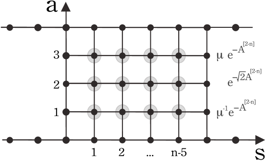
Figure 7: Strip where the $T$ and $Y$-functions live in the $AdS_{5}$ case. Small solid black dots represent $T$-functions. At the boundary the $T$-functions are equal to one except at the three nodes in the right boundary; there they take the values indicated in the figure. In all the points of the boundary the $Y$-functions are either zero or infinity. They are non-trivial in the smaller domain indicated by the fat shaded gray circles.

Next, we introduce the $Y$-functions

$$Y_{a,m}\equiv{T_{a,m+1}T_{4-a,m-1}\over T_{a+1,m}T_{a-1,m}}\,.$$ (47)

Being composed from next-to-nearest-neighbor $T$-functions, the $Y$-functions $Y_{a,s}$ are finite in a slightly smaller lattice parametrized by $a=1,2,3$ and $s=1,\dots,n-5$. The number of $Y$-functions coincides with the number of independent cross ratios. The Hirota equation then implies the following Y-system for these quantities:

$${Y_{2,m}^{-}Y_{2,m}^{+}\over Y_{1,m}Y_{3,m}} = {(1+Y_{2,m+1})(1+Y_{2,m-1})\over(1+Y_{1,m})(1+Y_{3,m})}$$

$${Y_{3,m}^{-}Y_{1,m}^{+}\over Y_{2,m}} = {(1+Y_{3,m+1})(1+Y_{1,m-1})\over 1+Y_{2,m}}$$ (48)

$${Y_{1,m}^{-}Y_{3,m}^{+}\over Y_{2,m}} = {(1+Y_{1,m+1})(1+Y_{3,m-1})\over 1+Y_{2,m}}$$

or in a more compact notation

$${Y_{a,m}^{-}Y_{4-a,m}^{+}\over Y_{a+1,m}Y_{a-1,m}} = {(1+Y_{a,m+1})(1+Y_{4-a,m-1})\over(1+Y_{a+1,m})(1+Y_{a-1,m})}\,\,\,\,\,,\,\,\,\,\,\begin{array}[]{l}a=1,2,3\,,\\ s=1,\dots,n-5\end{array}$$ (51)

To recover (48) we need to use that $Y_{0,s}=Y_{4,s}=\infty$.

4.3 Analytic properties of the $Y$-functions

To derive the integral form of the Y-system equations it is important to identify the large $\theta$ asymptotics. They are fixed by a WKB analysis. The method is very similar to the one used for the $AdS_{3}$ case, but a bit more involved. We will leave the details for appendix E and state here the final results.

We choose the polynomial $P$ to be such that all zeros are on the real axis and $P(z)>0$ for sufficiently large $z$. Then the large $\theta$ behavior of the $Y$-functions is

$$\log Y_{1,s}\to-m_{s}\cosh\theta-C_{s}\pm D_{s}\,\,\,,\,\,\,\theta\to\pm\infty$$

$$\log Y_{3,s}\to-m_{s}\cosh\theta+C_{s}\mp D_{s}\,\,\,,\,\,\,\theta\to\pm\infty$$ (52)

$$\log Y_{2,s}\to-\sqrt{2}\,m_{s}\cosh\theta\leavevmode\nobreak\ ,\leavevmode\nobreak\ \leavevmode\nobreak\ \leavevmode\nobreak\ \leavevmode\nobreak\ \leavevmode\nobreak\ \leavevmode\nobreak\ \,\,\,\,\,\,\theta\to\pm\infty$$

where $\theta=\log(\zeta)$. The constants $C_{s}$ and $D_{s}$ arise from the components of the connection $A$ that survive the $Z_{4}$ projection. For loops in signature $(1,3)$ or $(3,1)$ the $D_{s}$’s are real while the $C_{s}$’s are purely imaginary, see appendix F. In fact, we have the general reality condition

$$\left(Y_{a,s}(\zeta)\right)^{*}=Y_{4-a,s}(1/\zeta^{*})$$

In particular, for large $\theta=\log\zeta$, we see that

$$\left[\log\left(Y_{1,s}/Y_{3,s}\right)(+\infty)\right]^{*}=-\log\left(Y_{1,s}/Y_{3,s}\right)(-\infty)$$

which indeed implies what we said above regarding $D_{s}$ and $C_{s}$. It turns out that the $m_{s}$ can be promoted to complex constants by changing the position of the zeros of the polynomial. These $n-3$ complex constants, together with the purely imaginary $C_{s}$, constitute the $3(n-5)$ parameters of the problem.

4.4 TBA equations in $AdS_{5}$

To derive a set of integral equations from the functional Y-system we follow again the same route as in the $AdS_{3}$ case. As explained in the $AdS_{3}$ case, a big advantage of the integral form of the Y-system equations is the straightforward numerical implementation of these equations. We first consider the case where all masses are real and positive. We then introduce a set of functions $l_{a,s}=\log(Y_{a,s})+m_{a,s}\cosh\theta$ which are meromorphic in the strip $-\pi/4<Im(\theta)<\pi/4$ and bounded as we approach infinity inside this strip. Let us first assume that these functions are actually holomorphic in the strip and then we will mention what happens when there are poles. Equally important they obey

$$l_{a,s}^{+}+l_{4-a,s}^{-}-l_{a+1,s}-l_{a-1,s}=\log Y_{a,s}^{+}+\log Y_{4-a,s}^{-}-\log Y_{a+1,s}-\log Y_{a-1,s}\,.$$

The right hand side of this equality is the logarithm of the left hand side of the Y-system functional equations (48) derived above. Now we go to Fourier space where we have

$${\cal F}(l_{a,s}^{\pm})(\omega)=e^{\mp\frac{\pi\omega}{4}}{\cal F}(l_{a,s})(\omega)$$

where ${\cal F}$ denotes the Fourier transform. When writing this relation we are making use of the analytic properties of $l_{a,s}$ mentioned above. The $Y$-system equations can then be cast as

$$A_{aa^{\prime}}(\omega){\cal F}(l_{a^{\prime},s})(\omega)={\cal F}\left(\log\frac{(1+Y_{a,s+1})(1+Y_{4-a,s-1})}{(1+Y_{a-1,s})(1+Y_{a+1,s})}\right)(\omega)$$

For $w\neq 0$, the $3\times 3$ matrix $A_{aa^{\prime}}(\omega)$ is invertible and we can multiply this relation by $A^{-1}(w)$ to extract ${\cal F}(l_{a,s})$. For $w=0$ the matrix is not invertible and therefore when doing this operation we should allow for the constant zero modes in the final result. Finally, we rewrite the corresponding expression for ${\cal F}(l_{a,s})$ in position space. We obtain in this way the final set of integral equations

$$\log Y_{2,s} = -m_{s}\sqrt{2}\cosh\theta-K_{2}\star\alpha_{s}-K_{1}\star\beta_{s}$$

$$\log Y_{1,s} = -m_{s}\cosh\theta-C_{s}-\frac{1}{2}K_{2}\star\beta_{s}-K_{1}\star\alpha_{s}-\frac{1}{2}K_{3}\star\gamma_{s}$$ (53)

$$\log Y_{3,s} = -m_{s}\cosh\theta+C_{s}-\frac{1}{2}K_{2}\star\beta_{s}-K_{1}\star\alpha_{s}+\frac{1}{2}K_{3}\star\gamma_{s}$$

where $\alpha,\beta,\gamma$ are short-hand for

$$\alpha_{s}\equiv\log\frac{\left(1+Y_{1,s}\right)\left(1+Y_{3,s}\right)}{\left(1+Y_{2,s-1}\right)\left(1+Y_{2,s+1}\right)}\,\,,\,\,\gamma_{s}\equiv\log\frac{\left(1+Y_{1,s-1}\right)\left(1+Y_{3,s+1}\right)}{\left(1+Y_{1,s+1}\right)\left(1+Y_{3,s-1}\right)}\,,$$

$$\beta_{s}\equiv\log\frac{\left(1+Y_{2,s}\right)^{2}}{\left(1+Y_{1,s-1}\right)\left(1+Y_{1,s+1}\right)\left(1+Y_{3,s-1}\right)\left(1+Y_{3,s+1}\right)}\,,$$ (54)

and the kernels read

$$K_{1}\equiv\frac{1}{2\pi\cosh\theta}\,\,,\qquad K_{2}=\frac{\sqrt{2}\cosh\theta}{\pi\cosh 2\theta}\,\,,\qquad K_{3}=\frac{i}{\pi}\tanh 2\theta\,.$$

The unusual appearance of a kernel which does not decay at infinity ($K_{3}$) is a direct consequence of the singular behavior of $A(w)$ at $w=0$.

Comparing the large $\theta$ asymptotics following from these equations with those predicted from the WKB analysis we see that the zero modes $C_{s}$ correspond precisely to the constants $C_{s}$ in (52) while the $D_{s}$ in the WKB asymptotics are given by $D_{s}=\frac{i}{\pi}\int d\theta\,\gamma_{s}(\theta)$.

A more straightforward exercise, compared with deriving the integral equations, is to check that they indeed yield the functional relations. To do so we simply compute the left hand side of the functional equations using the integral equations. When doing this we should use

$$f^{\pm}=f(\theta\pm i\pi/4\mp i0)$$

in order not to touch the lines where the kernels $K_{2}$ and $K_{3}$ become singular. Then, simple identities such as $K_{1}^{+}+K_{1}^{-}-K_{2}=0$ and $K_{2}^{+}+K_{2}^{-}-2K_{1}=\delta(\theta)$ eliminate all the kernels in the right hand side of the integral equations and the functional equations are indeed reproduced.

Up to now we have discussed the case where all masses are real and positive. To consider the case of complex masses $m_{s}=|m_{s}|e^{i\varphi_{s}}$, we proceed in exactly the same way as described in section 3.5 for the $AdS_{3}$ TBA. That is, for small phases $\varphi_{s}$ the integral equations take the same form as in (53) with

$$m_{s}\to|m_{s}|\leavevmode\nobreak\ ,\quad Y_{a,s}(\theta)\to Y_{a,s}(\theta+i\varphi_{s})\leavevmode\nobreak\ ,\quad K_{s,s^{\prime}}^{a,a^{\prime}}(\theta-\theta^{\prime})\to K_{s,s^{\prime}}^{a,a^{\prime}}(\theta-\theta^{\prime}+i\varphi_{s}-i\varphi_{s^{\prime}})\leavevmode\nobreak\ ,$$

where $K$ stands for the three different kernels. At $|\varphi_{s}-\varphi_{s+1}|=\pi/4,\pi/2,3\pi/4,\dots$ we pick the poles from the appropriate kernels (see section 4.7 and appendix B for illustration). All in all, the Y’s and therefore the area are continuous whereas the apparent jumps in the integral equations are just an issue of the choice of contour.

4.5 Simple combinations of $Y$ functions and $s_{n+1}\to s_{1}$ monodromies

When we normalize the solutions as in (39) it can happen that $s_{n+1}$ is not equal to $s_{1}$. Of course, they have to be proportional to each other. The proportionality constant is called a “formal monodrom”. For $n$ odd, this constant can be removed, by rescaling the solutions appropriately. For $n$ even, there is some non-trivial gauge invariant information in this constant. In fact, this non-trivial information is a particular combination of $Y$ functions which is particularly simple.

This is most interesting for $n=4k$ so let us consider that case first. We introduce three combinations of $Y$ functions

$$B_{1} = \left(Y_{1,n-5}Y_{2,n-6}Y_{1,n-7}\right)\left(Y_{3,n-9}Y_{2,n-10}Y_{3,n-11}\right)^{-1}\left(Y_{1,n-13}Y_{2,n-14}Y_{1,n-15}\right)\dots$$

$$B_{2} = (Y_{2,n-5}Y_{1,n-6}Y_{3,n-6}Y_{2,n-7})(Y_{2,n-9}Y_{1,n-10}Y_{3,n-10}Y_{2,n-11})^{-1}\dots$$

$$B_{3} = \left(Y_{3,n-5}Y_{2,n-6}Y_{3,n-7}\right)\left(Y_{1,n-9}Y_{2,n-10}Y_{1,n-11}\right)^{-1}\left(Y_{3,n-13}Y_{2,n-14}Y_{3,n-15}\right)\dots$$

They are the analogue of $B(\zeta)$, equation (23), in the $AdS_{3}$ case. The $Y$-system alone, without recurring to the definition of the $Y$-functions, implies the following equations for $B_{a}$:

$$\frac{B_{2}^{+}B_{2}^{-}}{B_{1}B_{3}}=\frac{B_{1}^{-}B_{3}^{+}}{B_{2}}=\frac{B^{-}_{3}B^{+}_{1}}{B_{2}}=1\,.$$

They have the form of a discrete Laplace equation for $\log(B_{a})$ with a non-diagonal metric. Given the expected analytic properties of this functions the solution to these equations is

$$B_{1}=\mu^{-1}\left(e^{-{w_{0}\over\zeta}-{\bar{w}}_{0}\zeta}\right)^{[-n+2]},\quad B_{2}=\left(e^{-\sqrt{2}({w_{0}\over\zeta}+{\bar{w}}_{0}\zeta)}\right)^{[-n+2]},\quad B_{3}=\mu\left(e^{-{w_{0}\over\zeta}-{\bar{w}}_{0}\zeta}\right)^{[-n+2]}$$

The value of $w_{0}$ can be found by computing the large $\theta$ asymptotics in the definiton of the $B_{a}$’s. We find that

$$w_{0}=(m_{n-5}+\sqrt{2}m_{n-6}+m_{n-7})-(m_{n-9}+\sqrt{2}m_{n-10}+m_{n-11})+\dots$$

is the cycle around infinity and $\bar{w}_{0}$ its complex conjugate. In our normalization these quantities turn out to be equal to $B_{a}=T_{a,n-4}$ hence we have not only derived the form (46) but we also computed $w_{0}$ from the $Y$-system equations.

For $n=4k+2$ we only have one simple combination which is

$$\prod\limits_{k=1}^{\frac{n-4}{2}}\frac{Y_{3,2k-1}}{Y_{1,2k-1}}=\mu^{2}\,.$$ (55)

This relation should be thought of as a gauge invariant definition of $\mu$. The fact that $\mu$ is constant also follows directly from the integral equations.

These relations imply some identities on the constants appearing in the WKB asymptotics. By considering the small and large $\zeta$ limit of (55) we find the expression for $\mu$ in terms of the $C_{s}$

$$\log\mu^{2}=\sum_{k=1}^{\frac{n-4}{2}}C_{2k-1}$$

In addition, we find a relation on the $D_{s}$ of the form

$$0=\sum_{k=1}^{\frac{n-4}{2}}D_{2k-1}$$ (56)

Note that we are viewing the $C_{s}$ as arbitrary constants, while the $D_{s}$ are determined by solving the integral equation. The results in this subsection can also be obtained by a direct analysis of the solutions at infinity, as is explained in appendix C.

4.6 Area and free energy

In this subsection we show that the area is related to the free energy of the TBA system. The final result is (64). The reader that is not interested in this derivation can jump to the final result.

Note that the area is independent of $\zeta$. However, our objective is to relate the cross ratios to the area. For this purpose, it is convenient to consider the small $\zeta$ expansion of the $Y$ functions. We have already encountered the small $\zeta$ expansion when we looked at the asymptotic conditions. This expansion can be viewed as a WKB expansion where $\zeta$ is playing the role of $\hbar$. We take complex masses but with small enough phases so that the WKB approximations that we did before continue to be valid, with the same choice of cyl For our purpose, we need to expand these functions to first order in $\zeta$. For small $\zeta$ we diagonalize $\Phi_{z}={\rm diag}(x_{i})$, where $x_{i}$ are roots of $det(\Phi_{z}-x)=0$. In our case, we have $x^{4}-P(z)=0$. The $x_{i}$ are different sheets of a Riemann surface over the $z$ plane. Hitchin’s equations imply that $A_{\bar{z}}$ is also diagonal in the same basis. By a diagonal gauge transformation we can set $A_{\bar{z}}\to 0$. In general, $A_{z}$ is not diagonal in this basis. To order $\zeta^{0}$, only the diagonal components are relevant. Let us call these diagonal components by $\alpha^{i}_{z}$. Again, we can think of $\alpha$ as a one form on the Riemann surface. This is a closed form $d\alpha=0$ due to Hitchin’s equations.

When we evaluate the cross ratios we will be evaluating integrals of the form

$$\langle i|U|i\rangle=\langle i|Pe^{-\int{x_{i}dz\over\zeta}+A_{z}dz+\zeta\Phi_{\bar{z}}d\bar{z}}|i\rangle$$ (57)

Here $U$ is the “evolution operator” taking us between two points in the $z$ plane. The states $|i\rangle$ indicate that we follow a given branch, since changing branches is suppressed by an exponential amount. In other words, in the WKB approximation, we are following the “ground state" and the excited states are integrated out and change the evolution (at order $\zeta$ and higher) of the ground state. Expanding to order $\zeta$ we find that (57) has the form

$$\log\langle i|U|i\rangle=-\left[\int{x_{i}dz\over\zeta}+\alpha^{i}_{z}dz+\zeta(u^{i}_{z}dz+u^{i}_{\bar{z}}d\bar{z})+o(\zeta^{2})\right]$$ (58)

where $u^{i}$ is a certain one form. This one form is closed because the connection is flat. The $u_{\bar{z}}$ components of this one form are simple, they only come from the diagonal components of $\Phi_{\bar{z}}$, $u^{i}_{\bar{z}}=\Phi_{\bar{z}}^{ii}$. The $u_{z}$ component comes from a term that involves the off diagonal components of $A_{z}$, but we will not need the explicit expression here.

Once we form cross ratios, we find integrals over closed cycles on the Riemman surface of certain closed one form forms. Thus we obtain

$$\log\widehat{Y}_{\gamma}=-\left[{\oint_{\gamma}xdz\over\zeta}+\oint_{\gamma}\alpha+\zeta\oint_{\gamma}u+o(\zeta^{2})\right]$$ (59)

where $\alpha$ and $u$ are viewed now as forms on the Riemann surface (in the $i^{\rm th}$ sheet they are $\alpha^{i}$ or $u^{i}$ respectively). Since they were constructed from a flat connection, we see that the quantities in (59) do not depend on the precise choice of contour within its cohomology class. Thus, we can view them as conserved quantities of the Hitchin equation. In fact, we could expand to higher powers in $\zeta$ and find extra conserved quantities, though (59) is enough for our purposes.

In the gauge where we diagonalize $\Phi_{z}$, we can rewrite the expression for the area as

$$A = \int d^{2}zTr[\Phi_{z}\Phi_{\bar{z}}]=\int d^{2}z\sum_{i}x_{i}\Phi_{\bar{z}}^{ii}={i\over 2}\int\sum_{i}x^{i}dz\wedge u^{i}_{\bar{z}}d\bar{z}$$

$$A = {i\over 2}\int\,xdz\wedge u=-{i\over 2}w_{\gamma,\gamma^{\prime}}\oint_{\gamma}xdz\oint_{\gamma^{\prime}}u$$ (60)

In the second line we expressed the integral as an integral over the Riemann surface. We then used a complete basis of cycles indexed by $\gamma$, and we used a formula that is valid when we integrate products of closed forms. Here $w_{\gamma,\gamma^{\prime}}$ is the inverse of the intersection form for the cycles $\langle\gamma,\gamma^{\prime}\rangle$. This step is valid when the number of cycles is even (odd number of gluons), otherwise we will not find an inverse. In our particular problem, we will choose the basis of cycles to consist of all the WKB cycles associated to the $Y_{a,s}$ functions. It is convenient to undo the shifts that define the $Y$ functions and define $\widehat{Y}_{a,s}$ functions which consist of various cross ratios evaluated at the same value of $\zeta$, see (D.2) in appendix D. We then do the WKB expansion for a $\zeta$ with phase $e^{i\pi/8}$, so that all the $\widehat{Y}_{a,s}$ are associated to a corresponding cycle.

It is useful to compute the small $\zeta$ expansion of the $\widehat{Y}_{a,s}$ functions from the integral equations. We obtain

$$\log\widehat{Y}_{a,s}={Z_{a,s}\over\zeta}+a_{a,s}+\zeta\left[\bar{Z}_{a,s}+M^{a,s;a^{\prime},s^{\prime}}\int{d\theta^{\prime}\over 2\pi}e^{-\theta^{\prime}}\log(1+\widehat{Y}_{a,s}(\theta^{\prime}))\right]$$ (61)

where $M^{a,s;a^{\prime},s^{\prime}}$, or $M^{\gamma,\gamma^{\prime}}$, is a certain matrix that results from the small $\zeta$ expansion of the integral equation for $\widehat{Y}_{a,s}$. By comparing (61) with (59) we can read off the values of $\oint_{\gamma_{a,s}}u$. We obtain

$$-\oint_{\gamma_{a,s}}xdz = Z_{a,s}$$

$$-\oint_{\gamma_{a,s}}u = \bar{Z}_{a,s}+M^{a,s;a^{\prime},s^{\prime}}\int{d\theta^{\prime}\over 2\pi}e^{-\theta^{\prime}}\log(1+\widehat{Y}_{a,s}(\theta^{\prime}))$$

When we insert these expressions in (60) we get two terms $A=A_{periods}+A_{free}$ which are equal to

$$A_{periods} = -{i\over 2}w_{\gamma,\gamma^{\prime}}Z_{\gamma}\bar{Z}_{\gamma^{\prime}}$$

$$A_{free} = -{i\over 2}Z_{\gamma}w_{\gamma,\gamma^{\prime}}M^{\gamma^{\prime},\gamma^{\prime\prime}}\int{d\theta^{\prime}\over 2\pi}e^{-\theta^{\prime}}\log(1+\widehat{Y}_{a,s}(\theta^{\prime}))$$

$$A_{free} = -2\sum_{a,s}\int{d\theta\over 2\pi}Z_{a,s}e^{-\theta}\log[1+\widehat{Y}_{a,s}(\theta)]$$ (62)

Here we have used that $Z_{\gamma}w_{\gamma,\gamma^{\prime}}M^{\gamma^{\prime},\gamma^{\prime\prime}}=-4iZ_{\gamma^{\prime\prime}}$ for our case, due to the relation between the $Z_{\gamma}$ (or $m_{a,s}$) with various values of $a$ implicit in (52). The matrix of cycle intersections is given in appendix E, figure 17. We can take the average of (62) with a similar expression which we obtain if we did the large $\zeta$ expansion to obtain

$$A_{free} = -\sum_{a,s}\int{d\theta\over 2\pi}[Z_{a,s}e^{-\theta}+\bar{Z}_{a,s}e^{\theta}]\log[1+\widehat{Y}_{a,s}(\theta)]$$ (63)

$$A_{free} = \sum_{s}\int{d\theta\over 2\pi}|m_{s}|\cosh\theta\log\left[(1+Y_{1,s})(1+Y_{3,s})(1+Y_{2,s})^{\sqrt{2}}\right](\theta+i\alpha_{s})$$ (64)

where $e^{i\alpha_{s}}$ is the phase of $m_{s}$. In the last equation we have written the final answer in terms of the $Y$ functions (as opposed to the $\widehat{Y}$ functions). We have also used the relation between $m_{s}$ and $Z_{a,s}$, implicit in (52) and explicit in appendix G.1, eqn. (106). The explicit value of $A_{periods}$ for in terms of the masses $m_{s}$ is given in appendix G.1.

One can give an alternative derivation of this formula in the spirit of the one given in [15] for the $n=6$ case. This alternative derivation starts with the observation that the area $A$ can be viewed as the generating function of transformations that change $\zeta$. This is the generating function when we define a Poisson bracket for the Hitchin system that makes $\Phi_{z}$ and $\Phi_{\bar{z}}$ conjugate variables and similarly for $A_{z}$ and $A_{\bar{z}}$. Then one uses that the $\widehat{Y}$ are variables whose Poisson brackets are computable and related to the cycle intersections. Finally one uses the integral equations as above to expand the $\widehat{Y}$ functions for small $\zeta$, to find the Poisson brackets of the quantities involved in this expansion. In this way one can check that the final expression for the area does indeed generate the desired transformation.

Note that if we view the Hitchin system as arising from an ${\cal N}=2$ supersymmetric theory, then the $Z_{4}$ projection that we had would break ${\cal N}=2$ to ${\cal N}=1$ supersymmetry. This ${\cal N}=1$ theory has a global symmetry for rotations of $\Phi_{z}$ and $\Phi_{\bar{z}}$ in opposite directions. The area is then the $D$ term potential (or momentum map) for this symmetry. This connection between a four dimensional supersymmetric theory and two dimensional quantum integrable models is in the spirit of [28]. It would be interesting to find the precise relation. Note however, that in our $AdS_{5}$ problem we do not have supersymmetry, we have integrability.

4.7 The geometrical meaning of the Y-functions

In the previous sections we saw how to determine the area of the minimal surfaces for a given choice of masses and chemical potentials in the $Y$-system equations. To identify which polygons correspond to a given choice of masses and chemical potentials we must compute the space-time cross ratios (10) for these solutions. This can be done by evaluating the $Y$-functions at special values of the spectral parameter as we explain in this section. In fact, the $Y$ functions themselves are cross ratios, but written in terms of somewhat exotic variables, introduced in [29], as we explain in the next subsection, 4.7.1. In subsection 4.7.2 we explain how to obtain the more conventional cross ratios defined in terms of distances between cusps.

4.7.1 Relation between the $Y$ functions and twistor cross ratios

As we explained in the introduction, we can recover the form of the coset representative, $g^{-1}$ by picking a set of independent solutions of the linear problem, see 4. In our case, this is a set of four solutions $\psi_{a}$ of the linear problem. Each of these solutions is a spinor and $a=1,2,3,4$ labels the solution number. We can orthonormalize them so that $g^{-1}$ is a proper group element. These solutions then determine the shape of the string worldsheet in spacetime. Rotations of the $a$ indices by a group element $g_{0}$ corresponds to the $SO(2,4)$ $AdS$ isometries, $g\to g_{0}g$. A given solution, say $\psi_{a}$, can be expanded in terms of four other solutions as

$$\psi_{a}=\lambda^{i}_{a}s_{i+2}+\eta^{i}_{a}s_{i+1}+\tilde{\eta}^{i}_{a}s_{i-1}+\hat{\eta}^{i}_{a}s_{i}$$ (65)

where $s_{i+2}$ is the big solution in the Stokes sector $i$, and $s_{i\pm 1}$ are the intermediate solutions in Stokes sector $i$. As we a go to infinity within this Stokes sector $s_{i+2}\to\infty$. Thus, this is the dominant solution and it determines the behavior of $g^{-1}$ and eventually, also for the spacetime solution. We can calculate $\lambda^{i}_{a}$ as

$$\lambda^{i}_{a}=\langle s_{i-1},s_{i},s_{i+1},\psi_{a}\rangle=\langle\bar{s}_{i},\psi_{a}\rangle$$ (66)

Here $\lambda^{i}$ is a spinor of the spacetime conformal group, which acts on the index $a$.

Now, imagine that we want to evaluate inner products of the $\lambda^{i}$. In these inner products we contract the $a$ indices of the four spinors with an $\epsilon$ symbol. Notice that these are indices transforming under global conformal transformations. We obtain

$$\langle\lambda^{i},\lambda^{j},\lambda^{k},\lambda^{l}\rangle=\epsilon^{a,b,c,d}\lambda^{i}_{a}\lambda^{j}_{b}\lambda^{k}_{c}\lambda^{l}_{c}=\langle\bar{s}_{i},\bar{s}_{j},\bar{s}_{k},\bar{s}_{l}\rangle$$

Here we have used that, by performing a local gauge transformation and a global transformation, we can set the $\psi_{\alpha,a}=\delta_{\alpha,a}$ at some point on the worldsheet.

Using this formula plus the identities (93), (94) we can show that

$$\langle s_{i},s_{i+1},s_{j},s_{j+1}\rangle = \langle\lambda^{i},\lambda^{i+1},\lambda^{j},\lambda^{j+1}\rangle$$

$$\langle\bar{s}_{i},s_{j}\rangle=\langle s_{i-1},s_{i},s_{i+1},s_{j}\rangle = \langle\lambda^{i},\lambda^{j-1},\lambda^{j},\lambda^{j+1}\rangle\equiv\langle\lambda^{i},\bar{\lambda}^{j}\rangle$$

where ${\bar{\lambda}}^{i}=\lambda^{i-1}\wedge\lambda^{i}\wedge\lambda^{i+1}$. Using these relations we can express the $Y$ functions in terms of the $\lambda^{i}$, which are spacetime quantities. These “momentum twistors" can be introduced just from the knowledge of the position of the cusps [29]. In order to introduce them, we only need to know that we have a null sided polygon. When we introduce the $\lambda^{i}$ from this latter point of view, the $\lambda^{i}$ are defined up to an overall rescaling. In (66) we have picked a particular normalization. However, in the final expressions for the $Y$ functions in terms of $\lambda$, the overall normalization of each $\lambda^{i}$ drops out, for the same reason that the overall normalization of the $s_{i}$ drops out. Each $\lambda^{i}$ is associated to a null side of the polygon, and a pair of consecutive $\lambda$s determine the position of the cusp $X^{i}_{ab}=\lambda^{i}_{[a}\lambda^{i+1}_{b]}$, where $X^{i}_{ab}$ are six coordinates defined up to a rescaling obeying $X^{2}=0$. Thus, they define a point on the boundary of $AdS$ space.

Note that the $Y_{1,s}$ and $Y_{3,s}$ only differ by $s\leftrightarrow\bar{s}$, or $\lambda\leftrightarrow\bar{\lambda}$, see appendix D. This operation is simply target space parity.

4.7.2 Traditional cross ratios from the $Y$ functions

In this subsection, we explain how to obtain traditional cross ratios from the $Y$ function. By a “traditional" cross ratio we mean one constructed from physical distances as in (10). These can be introduced via

$$U_{s}^{[r]}\equiv\left.1+{1\over Y_{2,s}}\right|_{\theta=i\pi r/4}=\left.{T_{2,s}^{+}T_{2,s}^{-}\over T_{2,s+1}T_{2,s-1}}\right|_{\theta=i\pi r/4}\,.$$

where we combined the definition of $Y$-function in terms of the $T$-functions with Hirota equation (43). This ratio has been constructed so that it only involves the functions $T_{2,s}$. These are determinants of four small solutions of the form $\langle s_{i}s_{i+1}s_{j}s_{j+1}\rangle$. We recall that the physical cross ratios are ratios of four such quantities (10). For example,

$$U_{2k-2}^{[0]}={\langle s_{-k},s_{-k+1},s_{k},s_{k+1}\rangle\langle s_{-k-1},s_{-k},s_{k-1},s_{k}\rangle\over\langle s_{-k-1},s_{-k},s_{k},s_{k+1}\rangle\langle s_{-k},s_{-k+1},s_{k-1},s_{k}\rangle}={{\bf x}_{-k,k}^{2}{\bf x}_{-k-1,k-1}^{2}\over{\bf x}_{-k-1,k}^{2}{\bf x}_{-k,k-1}^{2}}\leavevmode\nobreak\ ,$$ (67)

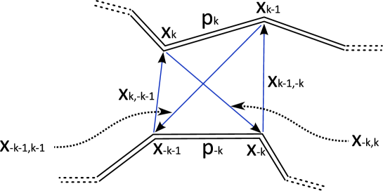
Figure 8: The cross ratio $U_{2k-2}^{[0]}={{\bf x}_{-k,k}^{2}{\bf x}_{-k-1,k-1}^{2}\over{\bf x}_{-k-1,k}^{2}{\bf x}_{-k,k-1}^{2}}$.

where ${\bf x}_{i,j}\equiv{\bf x}_{i}-{\bf x}_{j}$, see figure 8. If we consider $U_{2k-2}^{[2p]}$ then we will shift the position of the small solutions by $p$ sectors, i.e. we will get a cross ratio involving the cusps $\{{\bf x}_{-k-1+p},{\bf x}_{-k+p}\}$ and $\{{\bf x}_{k-1+p},{\bf x}_{k+p}\}$ of the polygon. We see that the index $2k-2$ is the number of cusps between ${\bf x}_{-k+p}$ and ${\bf x}_{k+p-1}$ (counted from the side of the cusp ${\bf x}_{0}$). Similarly, the cross ratio involving sides $\{{\bf x}_{-k-1+p},{\bf x}_{-k+p}\}$ and $\{{\bf x}_{k+p},{\bf x}_{k+1+p}\}$, which are separated by an odd number of cusps, are given by $U_{2k-1}^{[2p+1]}$.

A generic cross ratio involving four non-consecutive cusps of the polygon can easily be constructed by multiplying appropriate factors of $U_{s}^{[m]}$, e.g.

$${{\bf x}_{-2,1}^{2}{\bf x}_{-1,q+1}^{2}\over{\bf x}_{-2,q+1}^{2}{\bf x}_{-1,1}^{2}}=\prod_{l=1}^{q}U_{l}^{[l]}\,.$$

We see that once we solved the integral equations it suffices to evaluate the $Y$-functions $Y_{2,s}$ at some specific values of $\theta$ to read off the corresponding cross ratios.

A subtlety of pragmatic nature is the following. When solving the integral equation we usually do it numerically by iterating the integral equations. At the end of the iteration cycle we are left with the functions $Y_{a,s}(\theta)$ in the real axis which is precisely what we need to compute the free energy (64). On the other hand, to get the physical cross ratios we will generically need to evaluate $Y_{2,s}$ at some imaginary values. Using the integral equations, these cross ratios can be written in terms of (integrals of) the $Y$-functions evaluated in the real axis. When continuing the integral equations (53) out of the physical strip we will have to pick some extra pole contributions from the several kernels as we cross the lines ${\rm Im}(\theta)=\pm i\pi/4,\pm i\pi/2$ etc.

To make this procedure clear let us illustrate how to compute $Y_{2,s}(i\pi/2)$. First we notice that $Y_{a,s}\left(i\pi/4\right)$ can still be expressed in terms of integrals of the $Y$-functions over the real axis using the original undeformed equations (53). The only thing we must be careful about is that the kernels $K_{2}$ and $K_{3}$ have a pole singularity for $\theta=i\pi/4$ so that we should either interpret the integration contour to go slightly above the real axis or equivalently we should plug $\theta=i\pi/4-i0$ in the right hand side of these equations. To reach values of $\theta$ with an even larger imaginary part (such at $\theta=i\pi/2$) we can simply pick the pole singularities of these to kernels. For example

$$\log\left(Y_{2,s}\right)(\theta)=-m_{s}\sqrt{2}\cosh(\theta)-K_{2}\star\alpha_{s}-K_{1}\star\beta_{s}+\alpha_{s}(\theta-i\pi/4)\,\,\,,\,\,\,\pi/4<{\rm Im}(\theta)<\pi/2$$

We can now evaluate the right hand side of this equation at $i\pi/2-i0$ to compute $Y_{2,s}(i\pi/2)$. The last term becomes $\alpha_{s}(i\pi/4)$ and contains a bunch of $Y$-functions evaluated at $\theta=i\pi/4$. We already explained how to get those in terms of integrals of the $Y$-functions in the real axis using the original equations. Hence we are done.

There is an even more efficient way of computing these cross ratios which goes as follows. Suppose we need some Y-function $Y_{a,s}(\theta)$ where $\theta$ is outside the physical strip, i.e. $|{\rm Im}(\theta)|>\pi/4$. For concreteness let us suppose ${\rm Im}(\theta)<-\pi/4$. Then, by repeatedly using the functional equations (51) as

$$Y_{a,m}={(1+Y_{a,m+1}^{[1]})(1+Y_{4-a,m-1}^{[1]})\over Y_{4-a,m}^{[2]}(1+1/Y_{a+1,m}^{[1]})(1+1/Y_{a-1,m}^{[1]})}\,,$$

we can express $Y_{a,s}(\theta)$ purely in terms of $Y$-functions inside the physical strip. For those we can use the original integral equations (53) as explained above.

4.7.3 $\zeta$ symmetry

We explained how to get the physical cross ratios by evaluating the $Y$-functions at $\theta=0,\pm i\pi/4,\pm i\pi/2$ etc. Actually we can construct a family of polygons parametrized by a complex number $\theta_{0}$ which will all have the same area! These polygons are obtained by evaluating the $Y$-functions at $\theta=\theta_{0},\theta_{0}\pm i\pi/4,\theta_{0}\pm i\pi/2$ etc. The reason why we can evaluate the $Y$-functions around any $\theta_{0}$ is that flat sections of the linear problem can be assembled into a physical solution for general $\zeta=e^{\theta_{0}}$ at not only for $\zeta=1$. For purely imaginary $\theta_{0}$ the new polygons are real, for generic $\theta_{0}$ they are complexified. Thus we can view changes of $\zeta$ as a symmetry of the problem. Namely, we have a one parameter family of polygons labeled by $\zeta$ which have the same area. It would be very interesting to understand this symmetry in greater detail and specially to see if/how it manifests itself at the quantum level.

Note that this is intimately related to the fact that changes in $\zeta$ are generated by the area when one defines a certain Poisson bracket that is natural in the theory of Hitchin systems [15]. This Poisson bracket is different from the one one gets from the sigma model [35].

4.8 High temperature limit

In this section we will focus on a particular kinematical regime. From the Y-system point of view we want to consider the limit when the $Y$-functions are approximately constant (in some large region of $\theta$). To find the constant values of the $Y$-functions we solve the $Y$-system equations (51) and (55) dropping the $\zeta$ dependence, $Y_{a,s}^{\pm}\to Y_{a,s}$,

$${Y_{a,m}Y_{4-a,m}\over Y_{a+1,m}Y_{a-1,m}} = {(1+Y_{a,m+1})(1+Y_{4-a,m-1})\over(1+Y_{a+1,m})(1+Y_{a-1,m})}$$ (68)

For this approximation to be valid, the sources in the integral equations must become independent of the spectral parameter which means $m_{s}\to 0$. In the TBA context this arises in the high temperature limit, so will adopt that terminology here. Of course, in the $AdS$ problem there is no temperature since we are just solving classical equations. The $m_{s}\to 0$ condition is however not sufficient. Namely we do not have the freedom to chose the values of the constants $C_{s}$ if we want the solution to the Y-system to be given by constant $Y$-functions. Instead these constants are found from the $Y$-system. To derive this, note that the ratio of the equations (68) for $a=1$ and $a=3$ implies that $\gamma_{s}=0$ where $\gamma_{s}$ is defined in (54). Thus, from equations (53), we see that

$$e^{2C_{s}}={Y_{3,s}\over Y_{1,s}}\,.$$

We will first consider the richer case of an even number of gluons. The $n$ odd case is discussed afterwards. The equations (68) admit a one parameter family of solutions. We can parameterize this family in terms of

$$\prod\limits_{k=1}^{\frac{n-4}{2}}\frac{Y_{1,2k-1}}{Y_{3,2k-1}}=\frac{1}{\mu^{2}}\,.$$ (69)

For a fixed value of $\mu$, (68) admits a discreet set of solutions. At $\mu=1$ there is a unique solution such that $Y_{a,s}>0$ for any $a=1,2,3$ and $s=1,\dots,n-5$. We will consider a solution valid for arbitrary $\mu$ and continuously connected to that unique solution. This one parameter family describes a family of regular polygons with a $Z_{n}$ symmetry. This is shown in more detail in appendix I.

The polygon can be described in terms of the $n$ twistors

$$\bar{\lambda}_{k}=\{\left(1+a_{k}\right)(1+b_{k})e^{\frac{3i\pi k}{n}},(1+a_{k})e^{\frac{i\pi k}{n}},(1+b_{k})e^{-\frac{i\pi k}{n}},e^{-\frac{3i\pi k}{n}}\}$$ (70)

where $\mu=e^{i\phi}$ and

$$a_{k}=(-1)^{k}\tan\frac{2\pi}{n}\tan\frac{\phi}{n}\,\,\,,\,\,\,\qquad b_{k}=(-1)^{k}\tan\frac{\pi}{n}\tan\frac{\phi}{n}\,.$$

Then the constant solution to the $Y$-system is simply obtained by plugging the twistor $\bar{\lambda}_{k}$ in place of $s_{k}$ in the relations (96) in appendix D.

When $\phi=0$ we have $a_{k}=b_{k}=0$ and the solution simplifies to

$$Y_{a,s}+1=\frac{\sin\left(\frac{\pi}{n}\left(4-a+s\right)\right)\sin\left(\frac{\pi}{n}\left(a+s\right)\right)}{\sin\left(\frac{\pi}{n}\left(4-a\right)\right)\sin\left(a\frac{\pi}{n}\right)}\,\,.$$ (71)

Actually, in this case we have $Y_{a,s}=Y_{4-a,s}$ and hence the Y-system reduces to the standard $Y$-system and the solution (71) can be found in the literature [30]. In fact, this is a regular polygon that can be embedded in $AdS_{4}$. Another limit where we find significant simplification is the limit where $\phi\to\pi(n-4)/2$. In this limit we find $Y_{1,2k+1}=Y_{3,2k+1}=-1$, $Y_{1,2k}=Y_{3,2k}=0$, $Y_{2,2k+1}\to\infty$ and

$$Y_{2,2k}\to\sin\left(\pi\frac{k+2}{\hat{n}}\right)\sin\left(\pi\frac{k}{\hat{n}}\right)/\sin^{2}\left(\frac{\pi}{\hat{n}}\right)\,\,\,,\,\,\,\leavevmode\nobreak\ \leavevmode\nobreak\ \leavevmode\nobreak\ \leavevmode\nobreak\ \hat{n}\equiv{n\over 2}\,.$$ (72)

This corresponds to a regular polygon that can be embedded in $AdS_{3}$. In fact, the curious pattern of zeros and infinities for the $Y$-functions is a generic feature of the $AdS_{3}$ limit. In the next section 4.9, this is precisely how the $Y$-system in the $AdS_{5}$ strip reduces to the $Y$-system in the $AdS_{3}$ line. As we move $\phi$ between $\phi=0$ and $\phi={n-4\over 2}\pi$ we interpolate between these two cases.

It turns out that the free energy can be computed exactly in this limit, as shown for instance in [31], and reads

$$F_{n}=-\frac{1}{2\pi}\sum_{a,s}\left[\log(e^{(2-a)C_{s}}Y_{a,s})\log(1+Y_{a,s})+2Li_{2}(-Y_{a,s})\right]\leavevmode\nobreak\ .$$ (73)

Plugging the analytic expressions above into this expression we find the remarkably simple result

$$F_{n}=\frac{\pi}{2n}\left((n-4)(n-5)-\frac{4\phi^{2}}{\pi^{2}}\right)\,.$$ (74)

As already mentioned, for $\phi=0$ we recover the regular polygons of second class that can be embedded into $AdS_{4}$. One can actually see that the free energy for $\phi=0$ exactly reproduces the numerical prediction (110). Similarly, for $\phi=\frac{n-4}{2}\pi$ we can see that (74) exactly reproduces the $AdS_{3}$ result (111).

In addition to the solutions described above, there can be discrete families of solutions. For instance, let us focus in the $n$-odd case. In appendix I we have constructed a set of solutions parametrized by the number of sides $n$ and an extra integer $r$, with $r=2,...,(n-1)/2$. The spinors characterizing such solutions are

$$\lambda^{k}=(e^{i\pi(r+1)\frac{k}{n}},e^{i\pi(r-1)\frac{k}{n}},e^{-i\pi(r-1)\frac{k}{n}},e^{-i\pi(r+1)\frac{k}{n}})$$

where we have reorganized the expression appearing in the appendix. From these spinors, one can easily compute the cross-ratios $Y_{a,s}$. As these polygons can be embedded into $AdS_{4}$, we expect $\mu^{2}=1$ and indeed we find $\frac{Y_{1,s}}{Y_{3,s}}=1$. In addition, one can explicitly check that this cross-ratios give a solution of the $Y-$system equations. This constitutes a non trivial check of the $Y-$system for the case in which $n$ is odd.

Let us comment on an interesting feature of (74). Note that $\lambda$ in (70) is a periodic function of $\phi$ with period $n\pi$. This means that the cross-ratios describing the polygon are periodic functions of $\phi$. On the other hand we see that (74) is not periodic! We thus have a family of solution all ending on the same polygon. If the right prescription is to sum over all these surfaces, then the full result will have no monodromy. In that sum, one solution will dominate while the others are non-perturbative corrections (in $1/\sqrt{\lambda}$). On the other hand, in terms of amplitudes we expect non-trivial analytic continuation properties. For example, it is well known that amplitudes have interesting monodromies as we analytically continue the external parameters. This is an essential tool in weak coupling computations, see [32, 33] for example. If the right prescription is then not to sum over all these surfaces, then it would be interesting to study this particular kinematic configuration and understand in a better way the physical meaning of the monodromy in (74).

Such non-trivial monodromies for the free energy are a common occurrence in TBA systems. After an analytic continuation in the parameters we do not end up with the ground state, but we end up in an excited state [34]. In fact, the high temperature TBA typically corresponds to a CFT. Then the chemical potential simply translates into a winding condition for the scalar that bosonizes the corresponding $U(1)$ current and thus giving the $\phi^{2}$ contribution to the energy, see e.g. [36, 37]. This, in particular, shows that in our problem some excited states will typically appear as we analytically continue the parameter [36]. These are related to poles in the physical region and need to be taken into account according to a well understood procedure [34]. Namely, we need to deform the contours and pick up the corresponding poles, etc.

4.8.1 High temperature limit of $AdS_{3}$ $Y-$system

We can consider the high temperature limit of the TBA equations corresponding to scattering amplitudes on $AdS_{3}$ for $n=2\hat{n}$ gluons. In this case the $Y$-system equations (18) becomes simply $Y_{s}^{2}=(1+Y_{s+1})(1+Y_{s-1})$ and the constant solution reads

$$Y_{s}=\sin\left(\frac{\pi(s+2)}{\hat{n}}\right)\sin\left(\frac{\pi s}{\hat{n}}\right)/\sin^{2}\left(\frac{\pi}{\hat{n}}\right)$$

These are precisely the $Y$-functions found in the previous section in equation (72). This is not surprising since we had already anticipated that for $\phi\to(n-4)\pi/2$ the polygons described by the previous solution become $AdS_{3}$ solutions. The $AdS_{3}$ free energy can be then evaluated, exactly as in (73), and we obtain

$$F_{n}=-\frac{1}{2\pi}\sum_{s}\left[\log(Y_{s})\log(1+Y_{s})+2Li_{2}(-Y_{s})\right]=\pi\frac{(n-6)(n-4)}{12n}$$ (75)

where we have reinstated $n=2\hat{n}$. This result is however not the same as (74) for $\phi=(n-4)\pi/2$ even though we are describing the same solution. This is actually not a contradiction: as explained in appendix H the regularization of the area in the high temperature limit amounts to subtracting the area of $n-4$ regular pentagons in the $AdS_{5}$ case and the area of $n/2-2$ regular hexagons in the $AdS_{3}$ case. Taking this into account, the difference between two free energies is precisely as expected!

4.9 $AdS_{4}$ and $AdS_{3}$ reductions

Minimal surfaces that can be embedded in an $AdS_{4}$ or $AdS_{3}$ subspaces of $AdS_{5}$ are more restricted and as a result, the problem simplifies. The reduction of the $AdS_{5}$ flat connection was done in [15]. In this section, we will consider the implications of this simplification to the Y-system.

The worldsheet theory describing strings moving in an $AdS_{4}$ subspace is obtained from the parent $AdS_{5}$ by an additional projection. This projection relates ${\cal A}$ to ${\cal A}^{t}$ via a gauge transformation $F$. That gauge transformation therefore relates solutions to the problem with solutions to the inverse problem. More precisely we have $\bar{s}_{i}(\zeta)=Fs_{i}(\zeta)$, where in our normalization $\det(F)=1$. As a result, $Y_{1,s}=Y_{3,s}$ (and hence $\mu^{2}=1$). The $Y$-system equations can then be written in the form

$${Y_{2,m}^{-}Y_{2,m}^{+}\over Y_{1,m}^{2}}={(1+Y_{2,m+1})(1+Y_{2,m-1})\over(1+Y_{1,m})^{2}}\,\,,\qquad{Y_{1,m}^{-}Y_{1,m}^{+}\over Y_{2,m}}={(1+Y_{1,m+1})(1+Y_{1,m-1})\over 1+Y_{2,m}}\,.$$

A solution in $AdS_{4}$ that can be embedded in $AdS_{3}$ must have even number of gluons. The linear problem splits into two decoupled problem denoted by left and right problems in [17]. In an appropriate gauge we can write

$$s_{2k}=\left(\begin{array}[]{c}s_{R,k}\\ 0\\ \end{array}\right)\,,\qquad s_{2k+1}=\left(\begin{array}[]{c}0\\ s_{L,k+1}\\ \end{array}\right)$$

where $s_{L}$ and $s_{R}$ are the small solution of the left and right $AdS_{3}$ problems respectively. Because of this factorization the $T$-functions can be dramatically simplified. We choose a normalization where the $AdS_{3}$ solutions obey $\langle s_{L,i},s_{L,i+1}\rangle=1$, and the same for the right. The left and the right problems are related by a rotation in the spectral parameter $\langle s_{R,a},s_{R,b}\rangle=\langle s_{L,a},s_{L,b}\rangle^{[2]}$. We can use this relation to translate all inner products into inner products of the left problem. We also recall the definition, $T_{k}\equiv\langle s_{L,0},s_{L,k+1}\rangle^{[-2k-2]}$, of the Hirota functions for the $AdS_{3}$ problem in section 3.2. We then find that the the Hirota variables $T_{a,s}$ of the $AdS_{5}$ problem have the form

$$T_{1,2k+1}(\zeta) = 0\leavevmode\nobreak\ ,\leavevmode\nobreak\ \leavevmode\nobreak\ \leavevmode\nobreak\ \leavevmode\nobreak\ \leavevmode\nobreak\ \leavevmode\nobreak\ \leavevmode\nobreak\ \leavevmode\nobreak\ \leavevmode\nobreak\ \leavevmode\nobreak\ \leavevmode\nobreak\ \leavevmode\nobreak\ \leavevmode\nobreak\ T_{0,s}=T_{4,s}=-1\leavevmode\nobreak\ ,$$

$$T_{1,2k}(\zeta) = -\langle s_{L,0},s_{L,k+1}\rangle^{[-2k]}=-T_{k}^{[2]}\,,$$

$$T_{2,2k}(\zeta) = -\langle s_{R,0},s_{R,k+1}\rangle^{[-2k-1]}\langle s_{L,0},s_{L,k+1}\rangle^{[-2k-1]}=-T_{k}^{[3]}T_{k}^{[1]}\,\,,$$

$$T_{2,2k+1}(\zeta) = \langle s_{R,0},s_{R,k+1}\rangle^{[-2k-2]}\langle s_{L,0},s_{L,k+2}\rangle^{[-2k-2]}=T_{k}^{[2]}T_{k+1}^{[2]}\,,$$

and of course $T_{3,s}(\zeta)=T_{1,s}(\zeta)$.

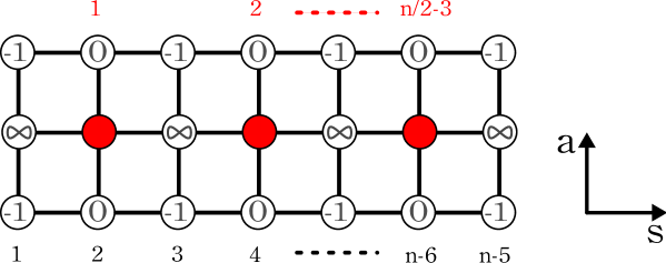
Figure 9: In the $AdS_{3}$ reduction most of the $3n-15$ functions $Y_{a,s}$ become trivial (either zero, one or infinity as indicated in the corresponding node in the figure). The $n/2-3$ nontrivial functions $Y_{2,2k}\equiv Y_{k}$ are indicated by red circles. The $AdS_{5}$ $Y$-system in the original strip (with shifts of $i\pi/4$) imply the $Y$-system equation for the line of red nodes $Y_{k}$ (with spectral parameter shifts of $i\pi/2$).

The $AdS_{5}$ Hirota equations (43) becomes identically satisfied in all nodes except $s=2k$ and $a=2$. For these, it becomes

$$\left(T_{k}\right)^{2}\left(T_{k}^{[2]}T_{k}^{[-2]}-T_{k-1}T_{k+1}-1\right)=0\leavevmode\nobreak\ ,$$

Inside the parentheses we recognize Hirota equation (16) in $AdS_{3}$. Recall that in the $AdS_{3}$ treatment supercripts denoted shifts in the spectral parameter which were twice as large compared to the ones we are using now, e.g.

$$\left(f^{[2]}\right)_{here}=\left(f^{+}\right)_{AdS_{3}\,\,section}\,.$$

The $3n-15$ nodes in the $AdS_{5}$ strip reduces to the $n/2-3$ nodes in the $AdS_{3}$ line in a very funny way which we represent in figure 9. Basically the only non-trivial functions become $Y_{2,2k}^{[-2]}=T_{k+1}T_{k-1}\equiv Y_{k}$ and these obey the $AdS_{3}$ Y-system equation (18).

5 Conclusions

In this paper we have given a way to compute the area of minimal surfaces that end on a null polygon at the boundary of $AdS_{5}$. The method uses the integrability of the classical equations in an essential fashion.

We have used the map between the integrable sigma model and a Hitchin system. The Hitchin system is an $SU(4)$, or $SU(2,2)$, or $SL(4)$ system depending on the signature. More precisely, it is a certain $Z_{4}$ projection of this system. Alternatively, we can simply say that we have chosen a specific form for the one parameter family of flat connections. This family is parametrized by a spectral parameter $\zeta=e^{\theta}$.

For this problem the worldsheet is the complex plane and we have an irregular singularity at infinity. This means that there are Stokes sectors as we approach infinity. Each of these Stokes sectors has an associated small solution $s_{i}$ and a large solution. The large solution determines a four-spinor $\lambda_{i}$, which specifies the direction in which the large solution is pointing. These spinors are associated to the sides of the polygon and are the same as the momentum twistors introduced by Hodges [29]. Alternatively, we can say that consecutive Stokes sectors determine a cusp or a vertex of the polygon. Using this cusp positions, or the momentum twistors $\lambda$, we can construct cross ratios. We can introduce a family of cross ratios depending on the spectral parameter $\zeta$. If $\zeta=1$ we recover the physical cross ratios of the original problem.

A particular set of cross ratios, denoted by the $Y$ functions $Y_{a,s}$, obeys a set of functional equations, or $Y$ system equations (51). The number of $Y$ functions is $3(n-5)$, which is the same as the number of independent cross ratios of the problem. These functional equations, together with some input regarding their asymptotic properties, imply a set of integral equations for the $Y_{a,s}$ functions (53). These integral equations involve $3(n-5)$ real parameters. These parameters were not present in the $Y$ system function equations but they appeared in the specification of the boundary conditions for the $Y$ functions. The solution to these equations relates these parameters to the physical cross ratios. Roughly speaking these parameters are related to the values of $Y$ at $\theta=\pm\infty$, while the physical cross ratios are $Y(\theta=1)$. These functional equations have the form of Thermodynamic Bethe Ansatz equations for a certain quantum system which is not associated in any obvious way to our initial problem, which was a classical problem. Similar relations were observed in [38]. Moreover, the area is given by the free energy of the TBA system. In practice, the TBA equations can be solved numerically. As in [15], we have been able to to solve the equations in a specific “high temperature” regime. This gives a one parameter family of solutions (for $n$ even). These describe a family of regular polygonal contours at the $AdS$ boundary. This is a one dimensional line in the $3(n-5)$ dimensional space of cross ratios. The answer for the area is surprisingly simple, it is just $A\propto\phi^{2}$, where $\phi$ parametrizes the family and it appears as a chemical potential of the TBA system. The cross ratios are periodic functions of $\phi$. This simple form is expected from the TBA perspective, since it is describing the UV limit of the 2d quantum integrable theory which is a CFT, and $\phi$ appears as a chemical potential [37]. One interesting aspect of this family of solutions is that, since we know it analytically, we can analytically continue in the space of parameters and find interesting monodromies. Namely, the cross ratios come back to themselves while the area does not. It would be interesting to study them further. One thing we can say, is that this shows that we will get TBA equations for excited states as we do analytic continuations. By now, this is a familiar phenomenon [34]. Thus the full problem involves not only the TBA ground state but also some excited states.

There are several interesting problems for the future. One of them is to take the large $n$ limit in order to obtain arbitrary (spacelike or timelike) contours. This would effectively solve the strong coupling form of the loop equations [41].

Of course, the most interesting open problem is the extension of this to the full quantum theory. This will probably require, as a first step, the knowledge of the classical solutions for the full $AdS_{5}\times S^{5}$ sigma model.

We have emphasized that we get the physical values of the cross ratios by evaluating the $Y$ functions at $\zeta=1$. However, we also get equally nice, but different, physical values by taking $\zeta=e^{i\varphi}$. By varying $\varphi$ we move in the space of cross ratios. All these values of the cross ratios have the same area!. Thus, changing $\zeta$ corresponds to a symmetry of the problem. Namely, by changing $\zeta$ we change the cross ratios in a way that does not change the area. Other values of $\zeta$, with $|\zeta|\not=1$ correspond to generically complex values of the cross ratios and represents an analytic continuation of the problem, an analytic continuation that keeps the area fixed. Recall also that, with a certain definition of Poisson brackets, the area is precisely the generating function for this symmetry [15].

One curious observation is the following. We have the formula for the amplitude as: Amplitude $=e^{-{\sqrt{\lambda}\over 2\pi}({\rm Area})}$. Since the area is the free energy, this formula looks like we are computing the partition function of the system on a torus, where one of the sides has length proportional to $\sqrt{\lambda}$. For large $\sqrt{\lambda}$ only the ground state contributes, which is what we computed. The overall sign is not quite right for this interpretation. It is nevertheless suggestive.

Appendix A Numerics

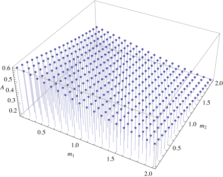
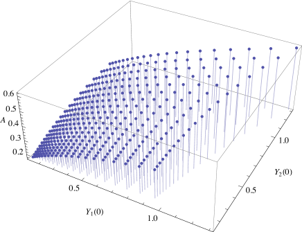
Figure 10: Left: Regularized area as a function of two real masses $m_{1}$ and $m_{2}$ for the decagon with $n=10$. When the masses are very large the $Y$-functions are exponentially suppressed and the free energy vanishes. When they are very small the free energy tends to the analytic prediction $F=\pi/5\simeq 0.63$ from the high temperature limit. Right: For those values of $m_{1}$ and $m_{2}$ the cross ratios $Y_{1}(0)$ and $Y_{2}(0)$ cover a diamond shaped region. The regularized area is plotted as function of these cross ratios.

In this section we explain how to implement equations (25) numerically in Mathematica in a very simple way (the code is quite similar to the one used in [42]). The algorithm is trivial, we simply iterate the integral equation plugging the $Y$-functions at iteration $k-1$ in the right hand side of (25) and reading from the left hand side their values at the $k$-th iteration. We start by defining the kernel appearing in the integral equations,

K[x_]=1/(2 Pi Cosh[x]);

and specify how many gluons we want to consider. We do that by introducing a list of masses which appear in the integral equations. For example, we set the following numerical values of the masses

m={1.,2.};M=Length[m];

would correspond to $M=2$ nodes, i.e. to a polygon with $2M+6=10$ sides. We also introduce a cut off for the several integrals and set the number of iterations,

cut = ArcCosh[8Log[10]/Min[m]]; ni = 8;

At each iteration step we compute the new values of the $Y$-functions at a discrete set of points and construct the new $Y$-function as the function which interpolates through these points. For that we need an interpolating function and a function to preform the several integrals ,

F[S_] := FunctionInterpolation[S,{x,-cut,cut}, InterpolationPoints->100]
int[S_] := NIntegrate[S,{y,-cut,cut}]/;NumberQ[S/.y->.1]

This is all the machinery we need. The iterations are simply implemented by

Y[a_,k_] := (0#&)/;a==0||a==M+1
Y[i_,1] := Exp[-m[[i]]Cosh[#]]&
Y[i_,k_] := Y[i,k] =
F[Exp[-m[[i]]Cosh[x]+int[K[x-y]Log[(1+Y[i-1,k-1][y])(1+Y[i+1,k-1][y])]]]]

In the first line we set $Y_{0}=Y_{M+1}=0$, in the second line we set the seed values for the iteration procedure to be simply the asymptotic expressions for the $Y$-functions and in the last command we compute the $Y$-functions at the iteration step $k$ using the right hand side of the integral equations with the $Y$-functions at step $k-1$. We can now compute the free energy from (3.6) and see how it converges to a particular value as we iterate:

energy=Table[int[Sum[Cosh[y]m[[i]]Log[1+Y[i,s][y]]/Pi/2,{i,M}]],{s,ni}]
ListPlot[energy]

For the masses chosen above we see that the free energy converges to $0.27$. Finally, if we want to read the cross-ratios of the polygon whose area we have just computed, we simply need to evaluate the $Y$-functions at $\theta=0$,

Table[Y[i,ni][0],{i,M}]

To compute the the free energy again for a different choice of masses we should first run Clear[Y].

The results of the numerics are shown for several values of $m_{1}$ and $m_{2}$ in figure 10. Here we have considered real values of $m_{1}$, $m_{2}$. One can similarly do computations for complex values of $m_{1},\leavevmode\nobreak\ m_{2}$, using the kernels after (26), and the discussion in appendix B, if necessary.

Appendix B Wall crossing and TBA

In this appendix we describe the pattern under which the $AdS_{3}$ integral equation (26) changes as the phases of the masses $\varphi_{s}=\arg(m_{s})$ are deformed beyond the region where $|\varphi_{s}-\varphi_{s+1}|<\pi/2$. The $AdS_{5}$ integral equations (53) follows an analogous pattern. In the context of the works [26, 25] this corresponds to the wall crossing phenomenon.

As explained in section 3.5, as long as $|\varphi_{s}-\varphi_{s+1}|<\pi/2$, the integral equation reads

$$\log\widetilde{Y}_{s}(\theta)=-|m_{s}|\cosh\theta+K_{s,s+1}\star\log(1+\widetilde{Y}_{s+1})+K_{s,s-1}\star\log(1+\widetilde{Y}_{s-1})$$ (76)

where $\widetilde{Y}_{s}(\theta)=Y_{s}(\theta+i\varphi_{s})$ and

$$K_{s,s^{\prime}}\star\log(1+\widetilde{Y}_{s^{\prime}})=\int{\log(1+\widetilde{Y}_{s^{\prime}}(\theta^{\prime}))\over 2\pi\cosh(\theta-\theta^{\prime}+i\varphi_{s,s^{\prime}})}d\theta^{\prime}$$

and $\varphi_{s,s\pm 1}\equiv\varphi_{s}-\varphi_{s\pm 1}$. Let us consider the simplest possible situation where $\varphi_{1,2}$ crosses the value $+\pi/2$ (and hence $\varphi_{2,1}$ crosses $-\pi/2$) while all other $|\varphi_{s,s+1}|<\pi/2$. Any other possibility can be treated similarly.

When $\varphi_{1,2}$ crosses the value $+\pi/2$ we pick the pole contribution from the kernel and the TBA equation for $s=1$ becomes

$$\log\widetilde{Y}_{1}(\theta)=-|m_{1}|\cosh\theta+K_{1,2}\star\log(1+\widetilde{Y}_{2})+\log(1+\widetilde{Y}^{\prime}_{2}(\theta))\leavevmode\nobreak\ ,$$ (77)

where

$$\widetilde{Y}^{\prime}_{2}(\theta)=\widetilde{Y}_{2}(\theta+i\varphi_{1,2}-i\pi/2)$$

is a “new" Y-function which arose in this process. Such $Y$-functions arise in pairs. Indeed, at the same time $\varphi_{2,1}$ crosses the the point $-\pi/2$, so that the equation for $\widetilde{Y}_{2}$ becomes

$$\log\widetilde{Y}_{2}(\theta)=-|m_{2}|\cosh\theta+\sum_{s=\{1,3\}}K_{2,s}\star\log(1+\widetilde{Y}_{s})+\log(1+\widetilde{Y}^{\prime}_{1}(\theta))\leavevmode\nobreak\ ,$$ (78)

where

$$\widetilde{Y}^{\prime}_{1}(\theta)=\widetilde{Y}_{1}(\theta+i\varphi_{2,1}+i\pi/2)\leavevmode\nobreak\ .$$

These equations are correct for $\pi/2<\varphi_{1,2}<\pi$. We evaluate (77) and (78) at $\theta\mp i(\varphi_{1,2}-\pi/2)\pm i0$ to get

$$\log\widetilde{Y}^{\prime}_{1}(\theta) = -|m_{1}|\cosh(\theta-i\varphi_{1,2}+i\pi/2)+\widetilde{K}_{1,2}\star\log(1+\widetilde{Y}_{2})+\log(1+\widetilde{Y}_{2}(\theta))$$ (79)

$$\log\widetilde{Y}^{\prime}_{2}(\theta) = -|m_{2}|\cosh(\theta+i\varphi_{1,2}-i\pi/2)+\sum_{s=\{1,3\}}\widetilde{K}_{2,s}\star\log(1+\widetilde{Y}_{s})+\log(1+\widetilde{Y}_{1}(\theta))\leavevmode\nobreak\ ,$$

where $\widetilde{K}$’s are the kernels shifted accordingly.

These equations, together with (77), (78) and (76) for $s>2$ constitute a closed set of $\hat{n}-1$ equations for the functions $\widetilde{Y}_{1},\widetilde{Y}_{2},\dots,\widetilde{Y}_{\hat{n}-3},\widetilde{Y}^{\prime}_{1},\widetilde{Y}^{\prime}_{2}$. If more phases become large we get in a similar way more extra functions $\widetilde{Y}^{\prime}_{s}$.

As usual in integrable models, nothing singular happens when the phases cross the values of $\pm\pi/2$ and new singularities hit the integration contour. After all the mechanism of picking the poles is precisely designed to keep everything smooth!. In particular there is no reason to change the expression of the area (3.6) which therefore keeps its form. Notice in particular that the tilded $Y$-functions are designed to be always exponentially suppressed as $\theta\to\pm\infty$.

Wall crossing in the $AdS_{5}$ system can be treated exactly in the same way.

B.1 Relation to Wall Crossing in [26]

In this same circumstance, the authors of [26] obtained only one extra function rather than two functions as we obtained above. This single extra function is associated to a new cycle on the Riemann surface (in the WKB approximation) which corresponds to $\gamma_{1+2}=\gamma_{1}+\gamma_{2}$. Thus, $Z_{1+2}=Z_{1}+Z_{2}$, or $m_{1+2}=m_{1}+im_{2}=|m_{1+2}|e^{i\varphi_{1+2}}$, where the $m_{i}$ are the complex $m$’s. In the language of [26] a new hypermultiplet has appeared.

In fact, we can define a new set of functions

$$\widetilde{Y}^{n}_{1}(\theta)={\widetilde{Y}_{1}\over 1+\widetilde{Y}_{2}^{\prime}}\leavevmode\nobreak\ ,\leavevmode\nobreak\ \leavevmode\nobreak\ \leavevmode\nobreak\ \leavevmode\nobreak\ \leavevmode\nobreak\ \leavevmode\nobreak\ \leavevmode\nobreak\ \widetilde{Y}^{n}_{2}={\widetilde{Y}_{2}\over 1+\widetilde{Y}^{\prime}_{1}}$$ (80)

$$\widetilde{Y}^{n}_{1+2}(\theta)={\widetilde{Y}_{1}(\theta+i\varphi_{1+2}-i\varphi_{1})\widetilde{Y}_{2}(\theta+i\varphi_{1+2}-i\varphi_{2}-i\pi/2)\over 1+\widetilde{Y}_{1}(\theta+i\varphi_{1+2}-i\varphi_{1})+\widetilde{Y}_{2}(\theta+i\varphi_{1+2}-i\varphi_{2}-i\pi/2)}$$ (81)

The first two variables are obviously designed to absorb the $\log(1+\widetilde{Y}^{\prime})$ terms in the right hand side of (77) (78). These relations look simpler when expressed in terms of the $Y$ functions (without the tildes)

$$Y^{n}_{1}={Y_{1}\over 1+Y_{2}^{-}}\leavevmode\nobreak\ ,\leavevmode\nobreak\ \leavevmode\nobreak\ \leavevmode\nobreak\ \leavevmode\nobreak\ \leavevmode\nobreak\ \leavevmode\nobreak\ \leavevmode\nobreak\ Y^{n}_{2}={Y_{2}\over 1+Y^{+}_{1}}\leavevmode\nobreak\ ,\leavevmode\nobreak\ \leavevmode\nobreak\ \leavevmode\nobreak\ \leavevmode\nobreak\ \leavevmode\nobreak\ \leavevmode\nobreak\ \leavevmode\nobreak\ \leavevmode\nobreak\ Y^{n}_{1+2}={Y_{1}Y_{2}^{-}\over 1+Y_{1}+Y_{2}^{-}}$$

where the $\pm$ index is the usual shift by $\pm i\pi/2$. The function $Y^{n}_{1+2}$ was defined so that

$$(1+Y_{1}) = (1+Y_{1}^{n})(1+Y_{1+2}^{n})$$ (82)

$$(1+Y_{2}) = (1+Y_{2}^{n})(1+Y_{1+2}^{n+})$$

which transforms (77) (78) into equations that look more like the equations in [26]

$$\log\widetilde{Y}^{n}_{1}=-|m_{1}|\cosh\theta+K_{1,2}\star\log(1+\widetilde{Y}^{n}_{2})+K^{+}_{1,1+2}\star\log(1+\widetilde{Y}^{n}_{1+2})$$

$$\log\widetilde{Y}^{n}_{2}=-|m_{1}|\cosh\theta+\sum_{s=1,3}K_{2,s}\star\log(1+\widetilde{Y}^{n}_{s})+K_{2,1+2}\star\log(1+\widetilde{Y}^{n}_{1+2})\leavevmode\nobreak\ ,$$

$$\log\widetilde{Y}_{3}=-|m_{3}|\cosh\theta+\sum_{s=2,4}K_{3,s}\star\log(1+\widetilde{Y}^{n}_{s})+K^{+}_{3,1+2}\star\log(1+\widetilde{Y}^{n}_{1+2})$$

where $Y_{s}^{n}=Y_{s}$ for $s>2$. The rest of the equations remains the same. Finally, the new equation for $\widetilde{Y}_{1+2}^{n}$ follows from considering the sum of (77) and (78) evaluated at the appropriate values, which are the ones in the numerator of (81). One of the kernels gives a delta function and produces a factor of $\log(1+\widetilde{Y}_{1+2}^{n})$. This combines with other terms to give

$$\log\widetilde{Y}^{n}_{1+2}(\theta) = -|m_{1}+im_{2}|\cosh\theta+K^{-}_{1+2,1}\star\log(1+\widetilde{Y}^{n}_{1})+K_{1+2,2}\star\log(1+\widetilde{Y}^{n}_{2})$$ (83)

$$+K^{-}_{1+2,3}\star\log(1+\widetilde{Y}_{3})$$

In the previous subsection, the equation for the free energy did not change, it was still given by $\widetilde{Y}_{1}$ and $\widetilde{Y}_{2}$, with no appearance of two extra functions $\widetilde{Y}_{1}^{\prime}$, $\widetilde{Y}_{2}^{\prime}$. Here, however, due to (82), we have a change in the expression of the free energy to

$$F\to F^{n}=\int{d\theta\over 2\pi}\cosh\theta\left[|m_{1}|\log(1+\widetilde{Y}_{1}^{n})+|m_{2}|\log(1+\widetilde{Y}_{2}^{n})+|m_{1}+im_{2}|\log(1+\widetilde{Y}_{1+2}^{n})\right]$$

plus the usual terms for $s>2$. From our point of view, it is not clear whether this way of writing the integral equation has any advantage with respect to the one we wrote above.

Appendix C Asymptotic behavior of the solutions at large $z$

In this appendix we prove some formulas that are necessary to derive the $AdS_{5}$ $Y$-system equations.

We will start by defining the small solutions $s_{i}$ and $\bar{s}_{i}$ in a certain normalization which simplifies some of the formulas. Of course, the final $Y$ system involves cross ratios and is independent of such normalization details. Up to a normalization, $s_{i}$ is a solution of $(d+{\cal A}(\zeta))s=0$ that is small in Stokes sector $i$. Similarly, $\bar{s}_{i}$ is a solution of $(d-{\cal A}^{t}(\zeta))\bar{s}=0$ which is small in Stokes sector $i$. Our first goal is to set a normalization of all these solutions so that (39) are valid.

It is convenient to introduce the $w$ “plane” via $dw=P^{1/4}dz$. For large $z$, or large $w$ we cover the $w$ plane $n/4$ times as we go around the $z$ plane, since for large $z$ we have $w\propto z^{n/4}$, where $n$ is the number of gluons.

Our boundary conditions for the connection are such that, for large $w$ the connection is

$$d+{\cal A}(\zeta)\sim d+{\rm diag}(1,-i,-1,i){dw\over\zeta}+{\rm diag}(1,i,-1,-i)\zeta d\bar{w}$$ (84)

We can now choose a basis of approximate solutions of the form

$$\psi_{1} = e^{-(w/\zeta+\bar{w}\zeta)}(1,0,0,0)^{t}$$

$$\psi_{2} = e^{-(-iw/\zeta+i\bar{w}\zeta)}(0,1,0,0)^{t}$$

$$\psi_{3} = e^{-(-w/\zeta-\bar{w}\zeta)}(0,0,1,0)^{t}$$ (85)

$$\psi_{4} = e^{-(iw/\zeta-i\bar{w}\zeta)}(0,0,0,1)^{t}$$

For zero phase of $\zeta$, the above solutions are the small solutions in consecutive sectors starting from the one centered on the positive real axis, followed by the one centered on the positive imaginary axis, and so on.

We normalize the small solutions $s_{i}$ by saying that $s_{i}=\psi_{a}$ with $a=i\,{\rm mod}(4)$ in the corresponding Stokes sector. Similarly, we choose a basis for the bar solutions

$$\bar{\psi}_{1} = e^{(w/\zeta+\bar{w}\zeta)}(1,0,0,0)^{t}$$

$$\bar{\psi}_{2} = e^{(-iw/\zeta+i\bar{w}\zeta)}(0,1,0,0)^{t}$$

$$\bar{\psi}_{3} = e^{(-w/\zeta-\bar{w}\zeta)}(0,0,1,0)^{t}$$

$$\bar{\psi}_{4} = e^{(iw/\zeta-i\bar{w}\zeta)}(0,0,0,1)^{t}$$

The normalization of $\bar{s}_{i}$ is fixed by setting

$$\bar{s}_{i}=\bar{\psi}_{a+2}\leavevmode\nobreak\ ,\leavevmode\nobreak\ \leavevmode\nobreak\ \leavevmode\nobreak\ \leavevmode\nobreak\ i=a+2\,\,{\rm mod}(4)$$

in the corresponding Stokes sector.

We can now check that

$$\langle s_{i},s_{i+1},s_{i+2},s_{i+3}\rangle=(-1)^{i+1}$$

by evaluating this expression at infinity in sectors $i+1$ or $i+2$ where the asymptotics (85) of all these small solutions are still reliable. Similarly,

$$\bar{s}_{i}=(-1)^{i+1}s_{i-1}\wedge s_{i}\wedge s_{i+1}$$ (86)

$$s_{k+1}(\zeta)=(\hat{C})^{T}\bar{s}_{k}(i\zeta)$$

$$\bar{s}_{k+1}(\zeta)=(\hat{C})^{-1}s_{k}(i\zeta)\leavevmode\nobreak\ ;\leavevmode\nobreak\ \leavevmode\nobreak\ \leavevmode\nobreak\ \leavevmode\nobreak\ \leavevmode\nobreak\ \leavevmode\nobreak\ \leavevmode\nobreak\ \leavevmode\nobreak\ \leavevmode\nobreak\ \leavevmode\nobreak\ \leavevmode\nobreak\ \leavevmode\nobreak\ \leavevmode\nobreak\ \leavevmode\nobreak\ \leavevmode\nobreak\ \leavevmode\nobreak\ \hat{C}^{-1}=\left(\begin{array}[]{cccc}\ 0&1&0&0\\ 0&0&1&0\\ 0&0&0&1\\ 1&0&0&0\end{array}\right)$$ (91)

This is not exactly as in the main text, so we perform a further redefinition of the small solutions

$$s_{4k+a}\to(-1)^{k}s_{4k+a}\leavevmode\nobreak\ ,\qquad\bar{s}_{4k+a+2}\to(-1)^{k}\bar{s}_{4k+a+2}\leavevmode\nobreak\ ,\qquad a=1,2,3,4\leavevmode\nobreak\ ,$$ (92)

This transforms the relations (86) into the ones in the main text (39). It also transforms the matrix $\hat{C}$ into the matrix $C$ in the main text, see (38), with ${\rm det}\,C=1$.

Using epsilon symbol identities one can check (easily with Mathematica) that

$$\langle\bar{s}_{k},\bar{s}_{k+1},\bar{s}_{j},\bar{s}_{j+1}\rangle=\langle s_{k},s_{k+1},s_{j},s_{j+1}\rangle$$ (93)

$$\langle\bar{s}_{k},\bar{s}_{k+1},\bar{s}_{k+2},\bar{s}_{m}\rangle=\langle s_{k+1},s_{m-1},s_{m},s_{m+1}\rangle$$ (94)

This identities, together with (39), imply that

$$\langle s_{k},s_{k+1},s_{j},s_{j+1}\rangle(\zeta) = \langle s_{k-1},s_{k},s_{j-1},s_{j}\rangle\left(e^{i\pi/2}\zeta\right)$$ (95)

$$\langle s_{j},\bar{s}_{k+1}\rangle(\zeta)=\langle s_{j},s_{k},s_{k+1},s_{k+2}\rangle(\zeta) = \langle s_{j},s_{j-1},s_{j-2},s_{k}\rangle(e^{i\pi/2}\zeta)=\langle\bar{s}_{j-1},s_{k}\rangle(e^{i\pi/2}\zeta)$$

These two relations are the important identities which we use in the main text. In deriving this relation one needs to use that if $U$ is any matrix with unit determinant, then the product of four solutions $\{Us_{i}\}$ is the same as the product of the four solutions $\{s_{i}\}$.

Let us conclude with some remarks about the monodromy when $i\to i+n$. Notice that if $n\not=4k$, then the solutions (85) appear to be misaligned after $i\to i+n$. This is not a problem because they are on different sheets which are connected by suitable powers of the matrix $C$. When $n=4k$ we can compare $s_{n+1}$ with $s_{1}$. In general, the $w$ variables are related by $w_{n+1}=w_{1}+w_{0}$. This expresses the fact that there is a logarithmic branch cut. This implies that there is a $\zeta$ dependent monodromy when we relate $s_{4k+a}\sim s_{a}e^{-i^{-a}w_{0}/\zeta-i^{a}w_{0}\zeta}$. If $n\not=4k$, then we can choose the origin of the $w$ plane so that there is no $\zeta$ dependent monodromy. Let us now worry about constant parts. These could arise as follows. In the $z$ plane we can have a gauge connection whose integral at large $z$ , $\oint A$, is non-zero (and proportional to the diagonal matrix ${\rm diag}(1,-1,1,-1)$). In writing (84) we have made a gauge transformation that sets it to zero. However, this gauge transformation is not globally well defined and it appears as an extra gauge transformation that we need to do when we relate $s_{n+1}$ with $s_{1}$. When $n$ is odd no such transformation is possible. In fact, it is easy to check that a change in normalization of the solutions of the form $s_{i}\to\gamma^{(-1)^{i}}s_{i}$ and $\bar{s}_{i}\to\gamma^{(-1)^{i+1}}\bar{s}_{i}$ can remove any constant from the relation between $s_{n+1}$ and $s_{1}$. In the case that $n$ is even, there can be a constant piece in the formal monodromy. We can take it to have the form $s_{n+i}=\mu^{(-1)^{i}}s_{i}$. This is present both for $n=4k$ and $n=4k+2$. In section 4.5, these properties were derived directly from the $Y$-system and the analytic properties.

Appendix D Explicit form of $T$ and $Y$-functions

In this appendix we summarize all $T$ and $Y$ functions of the $AdS_{5}$ problem. We use the shift identities (40) to bring the various inner products to the expressions below. In this appendix we use the notation $\langle s_{a}\bar{s}_{b}\rangle=\langle s_{a}s_{b-1}s_{b}s_{b+1}\rangle$ and $\langle\bar{s}_{b}s_{a}\rangle=\langle s_{b-1}s_{b}s_{b+1}s_{a}\rangle$ and drop commas inside angle brackets.

D.1 $T$-functions

$$T_{2,2k}^{-}=\langle s_{-k-2}s_{-k-1}s_{k}s_{k+1}\rangle\,\,,\,\,T_{2,2k+1}=\langle s_{-k-2}s_{-k-1}s_{k+1}s_{k+2}\rangle$$

$$T_{1,4l}=\langle\bar{s}_{-2l-1}s_{2l+1}\rangle\,\,,\,\,T_{1,4l+1}^{-}=\langle s_{-2l-2}\bar{s}_{2l+1}\rangle\,\,,\,\,T_{1,4l+2}=\langle s_{-2l-2}\bar{s}_{2l+2}\rangle\,\,,\,\,T_{1,4l+3}^{-}=\langle\bar{s}_{-2l-3}s_{2l+2}\rangle$$

$$T_{3,4l}=\langle s_{-2l-1}\bar{s}_{2l+1}\rangle\,\,,\,\,T_{3,4l+1}^{-}=\langle\bar{s}_{-2l-2}s_{2l+1}\rangle\,\,,\,\,T_{3,4l+2}=\langle\bar{s}_{-2l-2}s_{2l+2}\rangle\,\,,\,\,T_{3,4l+3}^{-}=\langle s_{-2l-3}\bar{s}_{2l+2}\rangle$$

Note the presence of some shifts in the left hand side. Note that $T_{1,s}$ and $T_{3,k}$ only differ by $s_{i}\leftrightarrow\bar{s}_{i}$.

D.2 $Y$-functions

$$Y_{2,2k}=\widehat{Y}_{2,2k}=\frac{\left\langle s_{-k-2}s_{-k-1}s_{k+1}s_{k+2}\right\rangle\left\langle s_{-k-1}s_{-k}s_{k}s_{k+1}\right\rangle}{\left\langle\bar{s}_{-k-1}s_{k+1}\right\rangle\left\langle s_{-k-1}\bar{s}_{k+1}\right\rangle}\,\,,$$ (96)

$$Y_{2,2k+1}^{-}=\widehat{Y}_{2,2k+1}=\frac{\left\langle s_{-k-3}s_{-k-2}s_{k+1}s_{k+2}\right\rangle\left\langle s_{-k-2}s_{-k-1}s_{k}s_{k+1}\right\rangle}{\left\langle\bar{s}_{-k-2}s_{k+1}\right\rangle\left\langle s_{-k-2}\bar{s}_{k+1}\right\rangle}\,\,,$$

$$Y_{1,4l+2}^{-}=\frac{\left\langle\bar{s}_{-2l-3}s_{2l+2}\right\rangle\left\langle\bar{s}_{-2l-2}s_{2l+1}\right\rangle}{\left\langle s_{-2l-4}\bar{s}_{-2l-2}\right\rangle\left\langle s_{-2l-3}s_{-2l-2}s_{2l+1}s_{2l+2}\right\rangle}\,\,\,\,\,\,\,\,\,,\,\,Y_{1,4l}^{-}=\frac{\left\langle s_{-2l-2}\bar{s}_{2l+1}\right\rangle\left\langle s_{-2l-1}\bar{s}_{2l}\right\rangle}{\left\langle s_{-2l-2}s_{-2l-1}s_{2l}s_{2l+1}\right\rangle\left\langle s_{2l-1}\bar{s}_{2l+1}\right\rangle}$$

$$Y_{1,4l+3}=\frac{\left\langle\bar{s}_{-2l-3}s_{2l+3}\right\rangle\left\langle\bar{s}_{-2l-2}s_{2l+2}\right\rangle}{\left\langle s_{-2l-4}\bar{s}_{-2l-2}\right\rangle\left\langle s_{-2l-3}s_{-2l-2}s_{2l+2}s_{2l+3}\right\rangle}\,\,\,\,,\,\,Y_{1,4l+1}=\frac{\left\langle s_{-2l-1}\bar{s}_{2l+1}\right\rangle\left\langle s_{-2l-2}\bar{s}_{2l+2}\right\rangle}{\left\langle s_{2l}\bar{s}_{2l+2}\right\rangle\left\langle s_{-2l-2}s_{-2l-1}s_{2l+1}s_{2l+2}\right\rangle}$$

$$Y_{3,4l+2}^{-}=\frac{\left\langle s_{-2l-3}\bar{s}_{2l+2}\right\rangle\left\langle s_{-2l-2}\bar{s}_{2l+1}\right\rangle}{\left\langle s_{-2l-3}s_{-2l-2}s_{2l+1}s_{2l+2}\right\rangle\left\langle s_{2l}\bar{s}_{2l+2}\right\rangle}\,\,\,\,\,\,\,\,\,\,\,\,\,\,\,\,,\,\,Y_{3,4l}^{-}=\frac{\left\langle\bar{s}_{-2l-2}s_{2l+1}\right\rangle\left\langle\bar{s}_{-2l-1}s_{2l}\right\rangle}{\left\langle s_{-2l-2}s_{-2l-1}s_{2l}s_{2l+1}\right\rangle\left\langle s_{-2l-3}\bar{s}_{-2l-1}\right\rangle}$$

$$Y_{3,4l+3}=\frac{\left\langle s_{-2l-3}\bar{s}_{2l+3}\right\rangle\left\langle s_{-2l-2}\bar{s}_{2l+2}\right\rangle}{\left\langle s_{-2l-3}s_{-2l-2}s_{2l+2}s_{2l+3}\right\rangle\left\langle s_{2l+1}\bar{s}_{2l+3}\right\rangle}\,,\,\,Y_{3,4l+1}=\frac{\left\langle\bar{s}_{-2l-1}s_{2l+1}\right\rangle\left\langle\bar{s}_{-2l-2}s_{2l+2}\right\rangle}{\left\langle s_{-2l-2}s_{-2l-1}s_{2l+1}s_{2l+2}\right\rangle\left\langle s_{-2l-3}\bar{s}_{-2l-1}\right\rangle}$$

We also define the functions $\widehat{Y}_{a,s}$ to be given by the right hand side of (D.2) without any extra shifts. In other words, $\widehat{Y}_{a,s}$ are defined as above with all the products defined at the same value of $\zeta$. In particular, we have included the explicit definitions of $Y_{2,s}$. These are related to spacetime cross ratios by replacing $s_{i}\to\bar{\lambda}_{i}$ and $\bar{s}_{i}\to\lambda_{i}$, where $\lambda_{i}$ are Hodges’ momentum twistor variables [29], see section 4.7.1.

Appendix E Asymptotic form of the $Y$ functions for the $AdS_{5}$ case

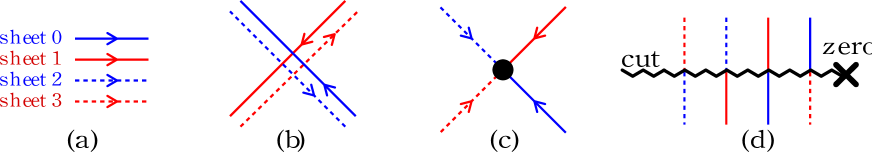
Figure 11: WKB lines for the $AdS_{5}$ case. We have four sheets. (a) Shows the conventions for naming the WKB lines for each of the four sheets. (b) Through a generic point we have four WKB lines passing. The red lines and the blue lines are orthogonal to each other . The line for the 1 sheet and the 3 sheet have opposite orientations and are on top of each other, here we have separated them for ease in visualization. (c) We evaluate an inner product of four solutions by bringing together four of the lines. The order of the lines indicates the sign, but we will not keep track of it. (d) When various WKB lines pass through a cut they change sheets according to the pattern here, the orientation of the line is preserved. If we have several zeros, the effects of this cuts add up.

In this appendix, we explain how to obtain the asymptotic form of the $Y$ functions for small $\zeta$. For small $\zeta$ we again diagonalize $\Phi_{z}\sim P^{1/4}{\rm diag}(1,-i,-1,i)$. We can then use a WKB approximation for the study of the solutions. At leading order the solutions are simply given by $\psi_{a}=\exp[-i^{-a}\int P(z)^{1/4}dz]$. We will follow WKB lines where the change of phase is real ${\rm Im}(i^{-a}P(z)^{1/4}\dot{z}/\zeta)=0$. This defines a family of lines. Here it is useful to think about this family of lines as lines on the Riemann surface, rather than lines on the $z$ plane. Of course, the Riemann surface is simply $x^{4}=P(z)$, and we have the differential $xdz=P(z)^{1/4}dz$. Different sheets of the Riemann surface are associated to different solutions of the linear problem. We label these sheets as $x_{a}$, $a=0,1,2,3$, in a cyclic way. We also have that $x_{a}=i^{-a}x_{0}$. The WKB lines have $Im(x_{a}\dot{z}/\zeta)=0$. They are oriented pointing towards the direction in which the solution increases. We label the WKB lines for different sheets by different types of lines in the $z$ plane, see figure 11(a). Of course, lines for the 1st and 3rd sheet coincide are oriented in the opposite way. Similarly for lines $0$ and $2$. Note, that we also want to keep track of the $\zeta$ independent part which comes from the connection $A$. The $A_{\bar{z}}$ component of the connection can be diagonalized and set to zero. Only the diagonal components of $A_{z}$ are relevant for the small $\zeta$ WKB approximation. These diagonal components are constrained by the $Z_{4}$ projection condition to be of the form

$$A_{z}=\alpha_{z}{\rm diag}(1,-1,1,-1)+\leavevmode\nobreak\ \leavevmode\nobreak\ {\rm off\leavevmode\nobreak\ diagonal\leavevmode\nobreak\ terms}$$ (97)

The off diagonal components are not relevant for us, since we are neglecting higher order terms in the small $\zeta$ expansion. Again we can think of $\alpha_{z}$ as a one form on the Riemann surface. The Hitchin equations imply that $d\alpha=0$. When we go around a zero of the Polynomial $P\sim(z-z_{0})$ we change sheets $x_{i}\to x_{i-1}$, see figure 11(d). Moreover, going around a zero, also $\alpha_{z}$ has a $Z_{2}$ branch cut, so that $\alpha_{z}\to-\alpha_{z}$. In other words, we really should think in terms of a $U(1)$ gauge field on the Riemann surface. The Riemann surface has a $Z_{4}$ symmetry $x\to ix$ and $\alpha$ is constrained to be odd under this symmetry.

The small solutions $s_{i}$ correspond to solutions that are associated to one of the sheets of the Riemann surface. In the large $z$ region the sheet of the Riemann surface associated to solution $s_{k}$ is simply $k\,{\rm mod}(4)$.

We will draw WKB lines associated to an inner product $\langle s_{i},s_{j},s_{k},s_{l}\rangle$ as four lines that are incoming if the product is in the numerator of the expression we want to evaluate. Each of the lines meeting at the inner produce lives on one of the four sheets, see figure 11(c). The lines start from each of the asymptotic regions associated to the corresponding Stokes sector and they end on the common point where the product is evaluated. We do this with WKB lines. Once we identify these lines we can move the point around on the Riemann surface in order to simplify the final expression. If the inner product is in the denominator, then we reverse the orientation of all the lines, without changing the sheet numbers.

We take a real polynomial with all its zeros on the real axis and with $P(z)>0$ for sufficiently large real $z$. We find it convenient to run all the cuts towards the left of the zero of the Polynomial $P$. The solution $s_{k}$ lives in sheet $k$ (modulo four). It is represented as a line coming in from infinity in the corresponding Stokes sector. These lines represent integration contours on the Riemann surface where we integrate both $P^{1/4}dz=xdz$ as well as $\alpha$.

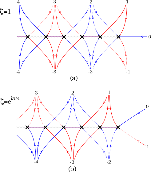
Figure 12: Schematic picture of the patterns of WKB lines for a Polynomial whose zeros are on the real axis. In (a) we show the pattern when the phase of $\zeta$ is 0 and in (b) we show it when the phase of $\zeta$ is $\pi/4$. Lines of different colors are supposed to be crossing at right angles. We have five lines ending at each zero. The purple line goes between two different zeros. (Its precise type depends on whether we put it above or below the cut). The $k^{\rm th}$ Stokes sector corresponds to a WKB line starting on sheet $k$. Notice that we have only drawn the lines that end at zeros. These lines are not useful for evaluating inner products but they are lines that separate different families of WKB lines. (The figures in this appendix are best viewed on a color monitor).

With all these preliminaries we are ready to start evaluating some cross ratios. We will evaluate some cross ratios when the phase of $\zeta$ is 1 and some where the phase of $\zeta=e^{i\pi/4}$. The patterns of WKB lines for our choice of polynomial for these two cases are given in figure 12. We could also alternatively evaluate them all at $\zeta=e^{i\pi/8}$ where the pattern of WKB lines is something intermediate between the patterns in figure 12.

It is convenient to redefine the $Y$ functions so that they all correspond to some cross ratios evaluated at the same value of $\zeta$. In other words, we define $\widehat{Y}_{a,s}$ which are given precisely by the expressions in the right hand side of formulas (96) , but with no shifts of the $\zeta$ argument in the left hand side. For instance, $\widehat{Y}_{2,2k}(\zeta)=Y_{2,2k}(\zeta)$ and $\widehat{Y}_{2,2k+1}(\zeta)=Y_{2,2k+1}^{-}$.

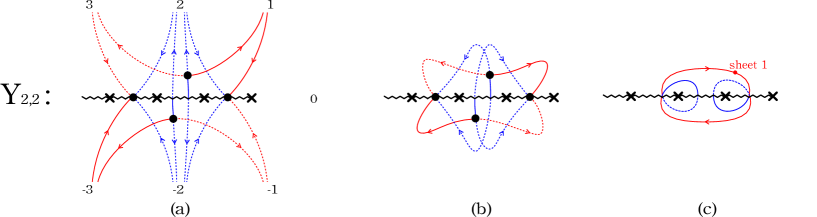
Figure 13: (a) We show the WKB lines that we use to evaluate the cross ratio $Y_{2,2}$. Each black dot corresponds to each inner product appearing in the cross ratio $Y_{2,2}$, see (98). The inner products that are in the numerator have incoming lines and the ones in the denominator have outgoing lines. We have set some dots right on the cuts, we could move them slightly up or down, and then we would indeed have four different types of lines ending on them. In (b) we have recombined the lines that we had in (a). In (c) we have moved the black dots around and we have “annihilated” them. We see the final cycle, $\gamma_{2,2}$ corresponding to $Y_{2,2}$. Note that the lines going between the two zeros are on the same sheet and have opposite orientations. Note also that $\alpha$ would be continuous through the cut going between the 2nd and 3rd zero. Thus there is no contribution from $\alpha$ to $Y_{2,2}$. For that reason, there is no constant term in (99).

Let us start with

$$\widehat{Y}_{2,2}=Y_{2,2}={\langle-3,-2,2,3\rangle\langle-2,-1,1,2\rangle\over\langle-3,-2,-1,2\rangle\langle-2,1,2,3\rangle}$$ (98)

Here we are using a short hand notation $\langle k,l,m,n\rangle\equiv\langle s_{k},s_{l},s_{m},s_{n}\rangle$. The WKB lines necessary to evaluate this quantity are displayed in figure 13(a). By reconnecting each pair of lines going in and out of an asymptotic region, we arrive at figure 13(b). Then, by bringing the four dots together and reconnecting lines on the same sheet and in the same orientation, we arrive to the closed contour drawn in figure 13(c).

Figure 14: In (a) and (b) we show the cycles $\gamma_{2,s}$ that correspond to the various $Y_{2,s}$ functions. We have indicated the sheet where the point with the dot is. Of course there are cuts emanating from the zeros, etc.

The procedure necessary to evaluate any of the $Y_{2,s}$ is basically the same and we get the contours displayed in figure 14. To evaluate $Y_{2,2k+1}$ we need to evaluate $\widehat{Y}_{2,2k+1}$ at $i\zeta$. The manipulations are identical, up to a relabeling of the solutions. For $\zeta$ real we can use the WKB lines that are associated to the pattern in 12(b). When we draw the contours in figure 14 we also note on which sheet they start. It is enough to label the sheet on which any point on the contour is, which determines the rest. It turns out that there is no contribution from the gauge connection $\alpha$ for this contour. We can see this by shrinking the little loops around the two zeros and then noticing that the two lines that go between the two zeroes in figure 14(c) are on the same sheet but have opposite orientation. In addition, we see that $\alpha$ is continuous across the cut joining the second and third zero in figure 14(c). This implies that the $\alpha$ dependent contribution vanishes.

In summary, this means that the $Y_{2,s}$ have the following behavior for small $s$.

$$\log\widehat{Y}_{2,s}={Z_{2s}\over\zeta}+o(\zeta)\leavevmode\nobreak\ \leavevmode\nobreak\ \leavevmode\nobreak\ \leavevmode\nobreak\ \leavevmode\nobreak\ \leavevmode\nobreak\ \leavevmode\nobreak\ \leavevmode\nobreak\ \leavevmode\nobreak\ \leavevmode\nobreak\ \leavevmode\nobreak\ \leavevmode\nobreak\ \leavevmode\nobreak\ Z_{2,s}=-\oint_{\gamma_{2,s}}xdz$$ (99)

where $\gamma_{2,s}$ are the cycles denoted in figure 14. Notice that the contours all look the same, except for the sheet they start on. ( As a first approximation the reader can ignore the subtlety about the sheet number where the contour starts.) The sheets change in such a way that $\log Y_{2,s}(\zeta=e^{\theta})\sim-{m_{2,s}e^{-\theta}\over 2}$ with $m_{2,s}$ real for our choice of the polynomial. Here $m_{2,s}$ are basically the $Z_{2,s}$ up to possible factors of $e^{i\pi/4}$ (for $s$ odd), see 106. In other words, if we consider one of the contours in figure 14, then the four different choices of the sheet it starts on would give four possible cycles on the Riemann surface. These would yield $Z_{2s},\leavevmode\nobreak\ iZ_{2,s},-Z_{2,s},-iZ_{2,s}$. The asymptotic behavior of $Y_{2,s}$ for $\zeta$ small and positive is governed by the cycle that renders $Y_{2,s}$ exponentially suppressed.

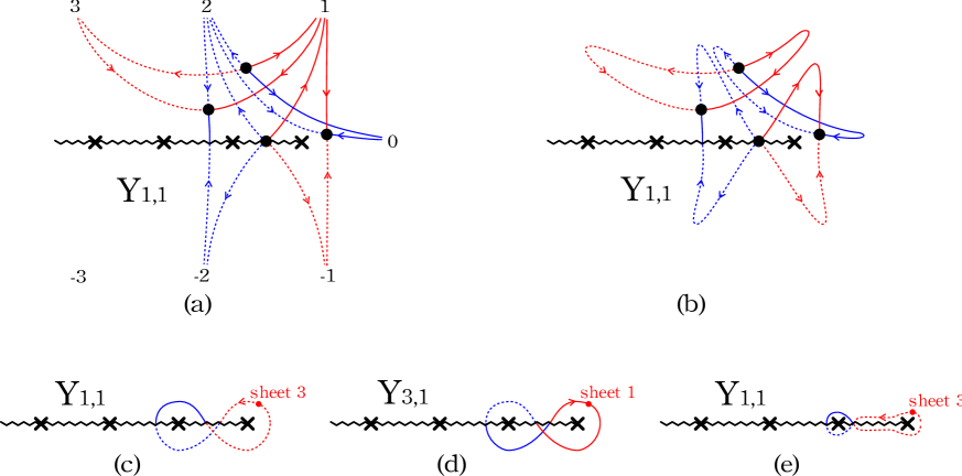
Figure 15: In (a) we show the WKB lines that are used for evaluating $Y_{1,1}$. In (b) we have reconnected the lines. In (c) we get the final cycle $\gamma_{1,1}$, which is the figure eight cycle indicated. In (d) we see the cycle we would have obtained if we had followed the same procedure for $Y_{3,1}$. We see that the cycles for $Y_{1,s}$ and $Y_{3,s}$ differ by a change in orientation and by a shift in sheet by two units. This does not affect the $\zeta$ dependent piece, but it changes the sign of the $\zeta$ independent piece coming from the gauge connection $\alpha$.

We can now evaluate one of the $Y_{1,s}$. Let us evaluate,

$$Y_{1,1}={\langle-2,{\bar{2}}\rangle\langle-1,\bar{1}\rangle\over\langle-2,-1,1,2\rangle\langle 0,1,2,3\rangle}={\langle-2,1,2,3\rangle\langle-1,0,1,2\rangle\over\langle-2,-1,1,2\rangle\langle 0,1,2,3\rangle}$$

The corresponding lines are drawn in figure 15(a). They can be reconnected as in figure 15(b). And finally lead to the figure eight contour in figure 15(c). It can be seen that there is an $\alpha$ dependent contribution to this contour. We can deform the contour to the one in figure 15(e). We see that the upper and lower parts of the contours really add, due to the properties of $\alpha$ as we cross a cut. Namely, $\alpha$ changes sign across the cut going between the first and second zero. This means that the upper and lower contributions of the contour add up and give a (generically) non zero answer for $a_{a,s}$. Finally, in figure 16 we draw the cycles $\gamma_{1,s}$ for $s=1,\dots,5$. They all have the same eight shape and differ by the sheet, orientation and zeros they encircle.

Figure 16: In (a) and (b) we show the cycles $\gamma_{1,s}$ that correspond to the various $Y_{1,s}$ functions. We have indicated the sheet where the point with the dot is. Of course, there are cuts emanating from the zeros, etc.

We can similarly evaluate

$$Y_{3,1}={\langle-\bar{2},{2}\rangle\langle-\bar{1},\bar{1}\rangle\over\langle-2,-1,1,2\rangle\langle 0,1,2,3\rangle}={\langle-3,-2,-1,2\rangle\langle-2,-1,0,1\rangle\over\langle-2,-1,1,2\rangle\langle 0,1,2,3\rangle}$$

Notice that this differs from $Y_{1,1}$ by an overall bar. This exchanges the top of the diagram in figure 16(a) with the bottom. The final contour is shown in figure 15(e). This differs from the one for $Y_{1,1}$ in figure 15(c) by the orientation and a change of sheets by two units. This combined operation does not change the integral of $xdz$, which contributes to the $1/\zeta$ term. However, it does reverse the sign of the contribution due to the gauge field $\alpha$.

Let us make a comment on the result for $Y_{a,s}$ as we vary $a$ for a given $s$. Notice that $Y_{1,s}$ is given by a figure eight contour, and so is $Y_{3,s}$, but with a different figure eight contour, e.g. see figure 15(c) and (d). In principle, the Riemann surface has four figure eight contours which start on different sheets. Our course, the sum is zero. In addition, we can have the sum of two consecutive figure eight contours. This sum can be deformed into the figure “double eight" contour that gives the result for $Y_{2,s}$. This implies the pattern of masses that we get for $Y_{a,s}$ for a given $s$.

In summary, we get

$$\log\widehat{Y}_{a,s}={Z_{\gamma_{a,s}}\over\zeta}+(a-2)c_{s}+o(\zeta)\leavevmode\nobreak\ ;\leavevmode\nobreak\ \leavevmode\nobreak\ \leavevmode\nobreak\ \leavevmode\nobreak\ \leavevmode\nobreak\ \leavevmode\nobreak\ \leavevmode\nobreak\ c_{s}=-\oint_{\gamma_{1,s}}\alpha$$ (100)

We also have that

$$Z_{\gamma_{1,s}}=Z_{\gamma_{3,s}}\leavevmode\nobreak\ ,\leavevmode\nobreak\ \leavevmode\nobreak\ \leavevmode\nobreak\ \leavevmode\nobreak\ \leavevmode\nobreak\ \leavevmode\nobreak\ \leavevmode\nobreak\ \leavevmode\nobreak\ \leavevmode\nobreak\ \leavevmode\nobreak\ \leavevmode\nobreak\ \leavevmode\nobreak\ Z_{\gamma_{2,s}}=(1-(-1)^{s}i)Z_{\gamma_{1,s}}$$ (101)

The last equality follows from the fact that the contours for $\widehat{Y}_{2,s}$ are a sum of two figure eight contours on neighboring sheets. Once we take into account the shifts in $\zeta$ in the definitions of $\widehat{Y}_{a,s}$ we see that (101) give the relations between the masses that we found in the $Y$-system.

It is interesting to compute the intersection form of all the cycles associated to the various Y functions. We get the result in figure 17. This result is used in section 3.6.

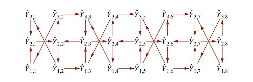
Figure 17: This figure shows the intersection form for all the cycles associated to the $Y$ functions. If an arrow points from $Y_{A}$ to $Y_{B}$ we have $\langle\gamma_{A},\gamma_{B}\rangle=1$ otherwise the intersection vanishes.

The analysis of the large $\zeta$ behavior is very similar to what we did above. We now diagonalize $\Phi_{\bar{z}}\to\bar{P}(\bar{z})^{1/4}(1,i,-1,i)$. We have the same pattern of WKB lines and the same cycles associated to the $\widehat{Y}_{a,s}$. But now we will be integrating $\bar{x}d\bar{z}$ to obtain $\bar{Z}_{\gamma_{a,s}}$. In addition, there is a contribution from the gauge connection $A$. In this case we can set $A_{z}=0$ and we focus on the diagonal part of the $A_{\bar{z}}$ connection, which is given in terms of a one form $\bar{\alpha}_{\bar{z}}$ on the Remann surface. We have then an expansion of the form

$$\log\widehat{Y}_{\gamma_{a,s}}={\bar{Z}_{\gamma_{a,s}}\zeta}+(a-2)\bar{c}_{s}+o(\zeta)$$

The constant parts $c_{s}$ in (100) and $\bar{c}_{s}$ are, in principle, different. They are constrained by the $Y$- system equation and we expect that, in the end, we have only one constant per value of $s$ which is actually a free parameter. This is most clear for low temperatures (or large values of the polynomial $P$). In this case, we can approximately simultaneously diagonalize $\Phi_{z}$ and $\Phi_{\bar{z}}$. As a result, $\alpha$ and $\bar{\alpha}$ coincide and $c_{s}=\bar{c}_{s}$ (see next appendix). As explained in the main text, in the general case, the average of these constants is a free parameter while the difference is determined by the equations.

Let us make a comment on the validity of the derivation of the WKB analysis. In this case, a given WKB curve gives a good approximation to the cross ratio in a region of size $\pi/2$ in $\zeta$ around the value of $\zeta$ for which the WKB curve exists. This is good enough for us to derive the $Y$-system, since we need displacements only of $\pi/4$. Note that the WKB curves exist for a range of $\zeta$ of total angle $\pi/2$ centered around the values where we did the computation. Thus, the total validity of the WKB analysis is a range of $\zeta$ of angle $\pi$ centered on real $\zeta$, for which we did the analysis. These remarks are valid as long as the polynomial has its zeros along the real axis.

When we move the zeros away from the real axis, the quantities $Z_{a,s}$ become more general complex numbers, though still constrained as in (101). Thus we have $2(n-5)$ complex parameters which correspond to the motion of the zeros of the polynomial. (There are other $(n-5)$ parameters in the constants $c_{s}+\bar{c}_{s}$). Now, as we move the zeros of the polynomial we will find that at some point some of the WKB lines will cease to exist. However, having derived the integral equation in one region in parameter space (i.e. for real masses), we can move to other regions by analytic continuation. In doing so, we have to change the integral equation according to an easily derived pattern, as explained in appendix B.

Appendix F Reality conditions for the $Y$ functions

The reality conditions for the $Y$ functions depend on the signature in which the solutions are embedded. More precisely, for $SO(p,6-p)$, they depend on the parity of $p$. For $p$ even, which corresponds to a boundary of $AdS$ with $(3,1)$ or $(1,3)$ signature, the reality conditions in a suitable choice of gauge have the form

$$A_{\bar{z}}^{\dagger}=-BA_{z}B^{-1}\leavevmode\nobreak\ ,\qquad\Phi_{\bar{z}}^{\dagger}=B\Phi_{z}B^{-1}\leavevmode\nobreak\ ,\leavevmode\nobreak\ \leavevmode\nobreak\ \leavevmode\nobreak\ \leavevmode\nobreak\ \leavevmode\nobreak\ \leavevmode\nobreak\ \leavevmode\nobreak\ \leavevmode\nobreak\ \leavevmode\nobreak\ \leavevmode\nobreak\ ({\cal A}(\zeta))^{\dagger}=-B{\cal A}(-{1\over\zeta^{*}})B^{-1}$$ (102)

For a suitable $B$ for each case. For $p$ odd, which for instance corresponds to the case of $(2,2)$ signature, the reality conditions have instead the form

$$A_{\bar{z}}^{*}=BA_{z}B^{-1}\leavevmode\nobreak\ ,\qquad\Phi_{\bar{z}}^{*}=B\Phi_{z}B^{-1}\leavevmode\nobreak\ ,\leavevmode\nobreak\ \leavevmode\nobreak\ \leavevmode\nobreak\ \leavevmode\nobreak\ \leavevmode\nobreak\ \leavevmode\nobreak\ \leavevmode\nobreak\ \leavevmode\nobreak\ \leavevmode\nobreak\ \leavevmode\nobreak\ ({\cal A}(\zeta))^{*}=B{\cal A}({1\over\zeta^{*}})B^{-1}$$ (103)

For a suitable $B$ for each case. The difference between different parities of $p$ comes from the fact that conjugation interchanges the spinorial and anti-spinorial representations for $p$ even, but it doesn’t for $p$ odd. In addition, we also have the $Z_{4}$ projection condition

$${\cal A}(i\zeta) = -C{\cal A}^{t}(\zeta)C^{-1}\leavevmode\nobreak\ ,\leavevmode\nobreak\ \leavevmode\nobreak\ \leavevmode\nobreak\ \leavevmode\nobreak\ \leavevmode\nobreak\ \leavevmode\nobreak\ \leavevmode\nobreak\ \leavevmode\nobreak\ \leavevmode\nobreak\ \leavevmode\nobreak\ \leavevmode\nobreak\ {\cal A}(-\zeta)=U^{-1}{\cal A}(\zeta)U\leavevmode\nobreak\ ,\leavevmode\nobreak\ \leavevmode\nobreak\ \leavevmode\nobreak\ \leavevmode\nobreak\ \leavevmode\nobreak\ \leavevmode\nobreak\ U=C^{t}C^{-1}$$ (104)

where the second equality arises by applying the first one twice.

Let us first focus in the case in which $p$ is even. If $\psi(\zeta)$ is a solution to $(d+{\cal A}(\zeta))\psi=0$, then by complex conjugating the above equation and using (102) (104) we get that

$$(d-{\cal A}^{t}(1/\zeta^{*}))D(\psi(\zeta))^{*}=0\leavevmode\nobreak\ ,\leavevmode\nobreak\ \leavevmode\nobreak\ \leavevmode\nobreak\ \leavevmode\nobreak\ \leavevmode\nobreak\ \leavevmode\nobreak\ \leavevmode\nobreak\ \leavevmode\nobreak\ \leavevmode\nobreak\ \leavevmode\nobreak\ \leavevmode\nobreak\ D=C^{-1}C^{t}B^{t}$$

This implies that $D(\psi(\zeta))^{*}\propto\bar{\psi}(1/\zeta^{*})$. If we take $\psi$ to be a small solution $s_{k}$, then we see that $(s_{k}(\zeta))^{*}\propto D^{-1}\bar{s}_{k}(1/\zeta^{*})$. Note that $D$ will drop out when we compute inner products, and any constant of proportionality drops out when we compute cross ratios. Thus the effect of performing a conjugation is to replace $s_{k}$ by $\bar{s}_{k}$ in all formulas. This implies that

$$\left(Y_{a,s}(\zeta)\right)^{*}=Y_{4-a,s}(1/\zeta^{*})$$

In particular, for large $\theta=\log\zeta$ we see that

$$\left[\log\left(Y_{1,s}/Y_{3,s}\right)(+\infty)\right]^{*}=-\log\left(Y_{1,s}/Y_{3,s}\right)(-\infty)$$

which implies that $c_{s}=-(\bar{c}_{s})^{*}$, or $C_{s}$ purely imaginary and $D_{s}$ purely real.

For $p$ odd the situation is different. By complex conjugating $(d+{\cal A}(\zeta))\psi(\zeta)=0$, and using (103), we simply obtain $(\psi(\zeta))^{*}\propto\psi(1/\zeta^{*})$. This implies $(s_{k}(\zeta))^{*}\propto s_{k}(1/\zeta^{*})$ and hence

$$\left(Y_{a,s}(\zeta)\right)^{*}=Y_{a,s}(1/\zeta^{*})$$

implying the $Y^{\prime}s$ are real when $\zeta$ is a phase. In this case $c_{s}^{*}=\bar{c}_{s}$, and $C_{s}$ is real and $D_{s}$ is purely imaginary.

Appendix G Components of the full area

As seen in the body of the paper, in order to compute scattering amplitudes at strong couplings, we need to compute the area of minimal surfaces in $AdS$, given by

$$A=\int d^{2}zTr\left[\Phi_{z}\Phi_{\bar{z}}\right]$$

Since for solutions relevant to scattering amplitudes, $Tr\left[\Phi_{z}\Phi_{\bar{z}}\right]\sim(P\bar{P})^{1/4}$, this area diverges and needs to be regularized. This can be conveniently done by dividing the area in different contributions (we refer the reader to [17, 15] for the details). Below we give the results for the case in which $n\neq 4k$, where the treatment is simpler

$$A = A_{reg}+A_{periods}+A_{cutoff}$$

$$A_{reg} = \int d^{2}z\left(Tr\left[\Phi_{z}\Phi_{\bar{z}}\right]-4(P\bar{P})^{1/4}\right)$$

$$A_{periods} = 4\int d^{2}z(P\bar{P})^{1/4}-4\int_{\Sigma_{0}}d^{2}w=4\int_{\Sigma}d^{2}w-4\int_{\Sigma_{0}}d^{2}w$$

$$A_{cutoff} = 4\int_{\sigma_{0},z_{AdS}>\epsilon}d^{2}w$$

where we have defined the $w-$plane by $dw=P(z)^{1/4}dz$. $A_{reg}$ is the non-trivial function that is computed by the free energy of the TBA equations and is the central quantity of this paper.

In $A_{periods}$, $\Sigma$ denotes the surface defined by the polynomial $P(z)$, while $\Sigma_{0}$ is a reference surface with a single branch point at the origin and the same structure at infinity. When computing it, it is important to use a cut-off in the $w-$plane, such as $|w|\leq\Lambda$, with $\Lambda\gg 1$. It can be evaluated in terms of the periods of the Riemann surface $x^{4}=P(z)$ and we give its explicit expression below.

When computing $A_{cut-off}$ we impose a physical cut-off, namely that the radial $AdS$ coordinate should be larger that certain small $\epsilon$. It can be conveniently written as the sum of two contributions

$$A_{cut-off}=\frac{1}{8}\sum_{i}\log^{2}(\epsilon^{2}{\bf x}_{i,i+2}^{2})+A_{BDS-like}$$

the first term is the standard divergent term, expected for light-like Wilson loops/amplitudes [43, 9]. The second term is

$$A_{BDS-like} = -\frac{1}{8}\sum_{\ell=1}^{n}\left(\log^{2}{\bf x}_{i,i+2}^{2}+\sum_{k=0}^{2K}(-1)^{k+1}\log{\bf x}_{i,i+2}^{2}\log{\bf x}_{i+2k+1,i+2k+3}^{2}\right),\leavevmode\nobreak\ \leavevmode\nobreak\ \leavevmode\nobreak\ n=4K+2$$

$$= -\frac{1}{4}\sum_{\ell=1}^{n}\left(\log^{2}{\bf x}_{i,i+2}^{2}+\sum_{k=0}^{2K}(-1)^{k+1}\log{\bf x}_{i,i+2}^{2}\log{\bf x}_{i+2k+1,i+2k+3}^{2}\right),\leavevmode\nobreak\ \leavevmode\nobreak\ \leavevmode\nobreak\ n=4K+2\pm 1$$

$A_{BDS-like}$ is a finite term which obeys the conformal Ward identities of broken conformal invariance [10] . Actually, it is the unique solution of the anomalous Ward identities that can be written only in terms of next to nearest distances ${\bf x}_{i,i+2}^{2}$.

It is customary to subtract the one loop result $A_{BDS}$ written down in [9], with the appropriate overall factor. As both, $A_{BDS-like}$ and $A_{BDS}$ satisfy the Ward identities, their difference is a function of the cross-ratios. In practise, in order to express $A_{BDS}-A_{BDS-like}$ in terms of cross-ratios, one simply starts with any non-next to nearest distance ${\bf x}_{i,j}^{2}$ appearing in $A_{BDS}$ and write it in terms of the unique cross-ratio $c_{i,j}$ which involves ${\bf x}_{i,j}^{2}$ and next to nearest distances ${\bf x}_{i,i+2}^{2}$. The strong coupling answer, however, organizes more naturally as described above.

G.1 Expression for $A_{periods}$

As already mentioned $A_{periods}$ can be evaluated in terms of the periods of the Riemann surface $x^{4}=P(z)$. More precisely, it is given by

$$A_{periods}=-\frac{i}{2}w_{\gamma,\gamma^{\prime}}Z_{\gamma}\bar{Z}_{\gamma^{\prime}}$$ (105)

where $\gamma$ denotes the collective pair $(a,s)$ and $w_{\gamma,\gamma^{\prime}}$ is the inverse of the intersection form of the cycles. Such inverse exists for the case in which $n$ is odd. Using the relation between the different periods and the relation between these and the masses

$$Z_{1,s}=Z_{3,s}\equiv Z_{s},\leavevmode\nobreak\ \leavevmode\nobreak\ \leavevmode\nobreak\ Z_{2,s}=(1-(-1)^{s}i)Z_{s}$$

$$m_{2s+1}=-2Z_{2s+1},\leavevmode\nobreak\ \leavevmode\nobreak\ \leavevmode\nobreak\ \leavevmode\nobreak\ \leavevmode\nobreak\ m_{2s}=-2e^{-\frac{i\pi}{4}}Z_{2s}$$ (106)

we can write $A_{periods}$ in terms of the masses of the TBA equations (53). We obtain

$$A_{periods}=\mathcal{K}_{ij}m_{i}\bar{m}_{j}$$

The form of $\mathcal{K}$ depends on the parity of $(n-1)/2$. For instance, for the case $n=4k+5$, $\mathcal{K}$ is a matrix of $4k$ by $4k$ and is equal to

$$\mathcal{K}=1_{k}\otimes\mathcal{K}_{1}+\mathcal{K}_{2}\otimes\mathcal{K}_{3}+\mathcal{K}_{2}^{T}\otimes\mathcal{K}_{3}^{T},\leavevmode\nobreak\ \leavevmode\nobreak\ \leavevmode\nobreak\ \leavevmode\nobreak\ \leavevmode\nobreak\ (\mathcal{K}_{2})_{i,j}=\theta(j-i)(-1)^{i-j+1},\leavevmode\nobreak\ \leavevmode\nobreak\ \leavevmode\nobreak\ \theta(0)=0$$ (107)

$$\mathcal{K}_{1}=-\frac{1}{\sqrt{2}}\left(\begin{matrix}0&\frac{1}{2}&\frac{1}{\sqrt{2}}&\frac{1}{2}\cr\frac{1}{2}&\frac{1}{\sqrt{2}}&1&\frac{1}{\sqrt{2}}\cr\frac{1}{\sqrt{2}}&1&\frac{1}{\sqrt{2}}&\frac{1}{2}\cr\frac{1}{2}&\frac{1}{\sqrt{2}}&\frac{1}{2}&0\end{matrix}\right),\leavevmode\nobreak\ \leavevmode\nobreak\ \leavevmode\nobreak\ \leavevmode\nobreak\ \mathcal{K}_{3}=\frac{1}{2\sqrt{2}}\left(\begin{matrix}0&1&\sqrt{2}&0\\ 0&\sqrt{2}&2&\sqrt{2}\\ 0&1&\sqrt{2}&1\\ 0&0&0&0\end{matrix}\right)$$

The case $n=4k+3$ has very similar expressions if we write $\mathcal{K}$ in terms of a $4k$ by $4k$ matrix whose last two rows and columns have to be chopped off. The expression coincides with that in (107), with different matrices $\mathcal{K}_{1}$ and $\mathcal{K}_{3}$

$$\mathcal{K}_{1}=\frac{1}{2\sqrt{2}}\left(\begin{matrix}\sqrt{2}&1&0&-1\\ 1&\sqrt{2}&0&-\sqrt{2}\\ 0&0&0&-1\\ -1&-\sqrt{2}&-1&0\end{matrix}\right),\leavevmode\nobreak\ \leavevmode\nobreak\ \leavevmode\nobreak\ \leavevmode\nobreak\ \mathcal{K}_{3}=-\frac{1}{2\sqrt{2}}\left(\begin{matrix}\sqrt{2}&1&0&-1\\ 2&\sqrt{2}&0&-\sqrt{2}\\ \sqrt{2}&1&0&-1\\ 0&0&0&0\end{matrix}\right)$$

The case $n=4k+2$ can be regarded as a limit of the case $n=4k+3$, in which we take one of the zeroes of the polynomial very far away. The correct prescription is to start with $A_{periods}^{4k+3}$, subtract $\frac{1}{2}(m_{4k-2}-\kappa)(\bar{m}_{4k-2}-\bar{\kappa})$ and then take $|m_{4k-2}|$ very large. $\kappa$ is then uniquely fixed by the requirement that linear divergences cancel. Again, the result can be written in exactly the form (107), with different matrices $\mathcal{K}_{1,3}$ and then chopping away the last three rows and columns

$$\mathcal{K}_{1}=-\frac{1}{4}\left(\begin{matrix}-1&0&1&\sqrt{2}\\ 0&0&\sqrt{2}&2\\ 1&\sqrt{2}&1&\sqrt{2}\\ \sqrt{2}&2&\sqrt{2}&0\end{matrix}\right),\leavevmode\nobreak\ \leavevmode\nobreak\ \leavevmode\nobreak\ \leavevmode\nobreak\ \mathcal{K}_{3}=-\frac{1}{4}\left(\begin{matrix}1&0&-1&-\sqrt{2}\\ \sqrt{2}&0&-\sqrt{2}&-2\\ 1&0&-1&-\sqrt{2}\\ 0&0&0&0\end{matrix}\right)$$

In particular, it can be checked that we reproduce the correct answer for the hexagon case [15].

The result for $A_{periods}$ is particularly simple in the case of $AdS_{3}$. It can be computed by using $A_{periods}^{AdS_{3}}=-iw_{rs}Z^{r}\bar{Z}^{s}$, but in this case the inverse matrix $w_{r,s}$ is much simpler. For $n=2\hat{n}$, gluons, with $\hat{n}$ odd, and defining $\tilde{m}_{2k}=m_{2k}$, $\tilde{m}_{1}=m_{1}$ and $\tilde{m}_{2k+1}=m_{2k-1}+m_{2k+1}$ for $k=1,...$, we obtain

$$A_{periods}^{AdS_{3}}=-\frac{1}{4}\sum_{k=1}^{\frac{\hat{n}-3}{2}}\left(\tilde{m}_{2k-1}\bar{\tilde{m}}_{2k}+\tilde{m}_{2k}\bar{\tilde{m}}_{2k-1}\right),\leavevmode\nobreak\ \leavevmode\nobreak\ \leavevmode\nobreak\ \leavevmode\nobreak\ \leavevmode\nobreak\$$ (108)

where we have used the relation between the periods $Z^{r}$ and the masses $m_{r}$ from section 3.

Appendix H Direct computation of the regularized area

In this appendix we consider the regularized area $A_{reg}$ for a particular class of regular polygons which can be embedded either in $AdS_{3}$ or $AdS_{4}$ and correspond to special radially symmetric solutions (in a sense which will be clear momentarily). We will then compare such results with the answer for the free energy of the Y-system in the high temperature limit.

We will be interested in the case of $(2,2)$ signature, since in this case we can embed both kind of solutions. Strings on $AdS_{4}$ can be described in terms of the usual holomorphic function $P(z)$ and two fields $\alpha$ and $\beta$. We can choose a gauge in which the connection becomes

$$A_{z}=\frac{1}{4}\left(\begin{matrix}-\partial\alpha-\partial\beta\sigma_{3}&0\\ 0&\partial\alpha-\partial\beta\sigma_{3}\end{matrix}\right),\leavevmode\nobreak\ \leavevmode\nobreak\ \leavevmode\nobreak\ \leavevmode\nobreak\ \Phi_{z}=-\left(\begin{matrix}0&e^{-1/2\alpha}\sqrt{2}P(z)^{1/2}\left(\begin{smallmatrix}0&e^{-1/2\beta}\cr e^{1/2\beta}&0\end{smallmatrix}\right)\\ \frac{e^{1/2\alpha}}{\sqrt{2}}&0\end{matrix}\right)$$

And $A_{\bar{z}}=-A_{z}^{\dagger}$, $\Phi_{\bar{z}}=\Phi_{z}^{\dagger}$. We have written the connection in terms of two by two blocks. We will consider a symmetric configuration in which all the zeroes of $P(z)$ are together, namely the holomorphic function is a homogeneous polynomial $P(z)\sim z^{n-4}$. In this limit, all its periods, and hence the masses entering the TBA equations, vanish. On the other hand, for this particular case, it is consistent with the equations of motion and boundary conditions to set $\alpha$ and $\beta$ to be functions of the radial coordinate only, $|z|$ or $|w|\equiv\rho$. It is convenient to write the equations they satisfy in the $w-$plane, defined by $dw=P(z)^{1/4}dz$

$$\hat{\alpha}^{\prime\prime}(\rho)+\frac{\hat{\alpha}^{\prime}(\rho)}{\rho}-8e^{\hat{\alpha}}+8e^{-\hat{\alpha}}\cosh\beta=0$$

$$\beta^{\prime\prime}(\rho)+\frac{\beta^{\prime}(\rho)}{\rho}-8e^{-\hat{\alpha}}\sinh\beta=0$$

where we have defined the shifted field $\hat{\alpha}=\alpha-\frac{1}{2}\log|P(z)|-\log 2$. For the scattering of $n$ gluons we will consider two different configurations. The first configuration, which exists only for $n$ even, corresponds to regular polygons that can be embedded into $AdS_{3}$ and hence $\beta=0$ for these. Geometrically, the span a regular polygon of $n$ sides in the $(x_{1},x_{2})$ plane and a segment in the $(t_{1},t_{2})$ plane, see figure 18 (a). They have been considered [17] and their area has already been computed there.

The second configuration corresponds to regular polygons that can be embedded into $AdS_{4}$. Geometrically, they have the shape of a regular polygon of $n$ sides in the $(x_{1},x_{2})$ plane and a regular polygon in the $(t_{1},t_{2})$ plane, of $n/2$ sides if $n$ is even, or $n$ sides if $n$ is odd, see figure 18 (b).

Figure 18: Two classes of regular polygons which live in $(2,2)$ signature and can be embedded in $AdS_{3}$ (a) and $AdS_{4}$ (b). Both posses a $Z_{n}$ symmetry.

As already mentioned, we expect $\hat{\alpha}$ and $\beta$ to be radially symmetric. Furthermore, following the discussion in appendix B of [15], we expect the following boundary conditions at the origin

$$\hat{\alpha}=2\frac{n-4}{n}\log\rho+c_{\alpha}+...$$

$$\beta=4\frac{n-4}{n}\log\rho+c_{\beta}+...$$

and a exponential decay at infinity. Finally, we are interested in the regularized area:

$$A_{reg}=2\pi n\int\rho d\rho(e^{\hat{\alpha}}-1)$$

It is at present unknown how to compute analytically the above area. Based on our experience with the first class of regular polygons, we expect a factor of $\pi$, times a simple rational function of $n$. Furthermore, this expression should vanish for $n=4$ and, in addition, we also know the correct value for $n=6$ from the results of [15].

We have solved the above equations numerically. The constants $c_{\alpha}$ and $c_{\beta}$ are unknown and are fixed by the constraint that the solutions decay at infinity. One should solve a shooting problem, trying several values for these constants approaching the correct ones by requiring that the solutions decay exponentially at infinity. We performed such procedure for $n=7,8$ and $n=10$ and obtained the following numerical results

$$A_{reg}^{n=7}\approx 4.882,\leavevmode\nobreak\ \leavevmode\nobreak\ \leavevmode\nobreak\ \leavevmode\nobreak\ \leavevmode\nobreak\ A_{reg}^{n=8}\approx 7.067,\leavevmode\nobreak\ \leavevmode\nobreak\ \leavevmode\nobreak\ \leavevmode\nobreak\ \leavevmode\nobreak\ A_{reg}^{n=10}\approx 11.85$$

Note that these expressions are well approximated by $\frac{87}{56}\pi,\frac{9}{4}\pi$ and $\frac{15}{4}\pi$. Once the regularized area is computed, in order to compare it to the free energy, we need to subtract an $n-$dependent constant, ensuring that the free energy vanishes for the situation in which all the zeroes are well separated. In this case, the regularized area approaches the quantity of zeroes, i.e. $n-4$, times the contribution of the regular pentagon, which corresponds to a single zero.

Extracting from [15] the value of the regularized area for the regular pentagon, $A_{penta}=\frac{3}{8}\pi$, we can give the final formula for the direct computation of the free energy

$$A_{free}=A_{reg}-(n-4)\frac{3}{8}\pi$$ (109)

From the numerical computations we can guess a very simple final formula for the regular polygons of the second class:

$$A_{free}^{(2)}=\frac{1}{2}\frac{(n-4)(n-5)}{n}\pi$$ (110)

This vanishes for $n=4$, as expected, gives the correct result for $n=6$ and agrees very well with the numerics for $n=7,8,10$.

Let us now plug in (109) the results for the regular polygons that can be embedded into $AdS_{3}$, read off from [17]. Substracting the appropriate contribution we obtain the appropriate quantity to be compared with the free energy for regular polygons of the first class:

$$A^{(1)}_{free} = A_{sinh}-(n-4)A_{pentagon}=-\pi\frac{n-4}{2n}\$$ (111)

where $A_{Sinh}$ is the result in [17]. We see that (111) vanishes for $n=4$, as expected, and also agrees with the answer of [15] for $n=6$.

$AdS_{3}$ limit

In the $AdS_{3}$ limit the expression for the regularized area of regular polygons is of course the same as for the polygons we were discussing above (which could be embedded $AdS_{3}$). However, in order to make a direct comparison with the free energy we need to substract a different contribution. Considering $n=2\hat{n}$ gluons, the holomorphic polynomial has $\hat{n}-2$ zeroes, each of which gives a contribution equal to that of the regular hexagon, we obtain:

$$A^{AdS_{3}}_{free} = A_{sinh}-(\hat{n}-2)\frac{7}{12}\pi=\pi{(n-6)(n-4)\over 12n}$$ (112)

Note that (112) is different from what we would obtain from the free energy in the $AdS_{5}$ case (111), due to the fact that we subtract different contributions.

Appendix I Regular polygons

In the body of the paper we have solved the TBA equations in the high-temperature limit, in which constant solutions of the Y-system are relevant. In this limit, and for an even number of sides, there is a family of solutions parametrized by a single parameter $\mu$. The solution interpolates between the two kind of regular polygons described in appendix H. In the following we describe the geometrical picture of such polygons. As we will see, this allows to compute analytic expressions for the various cross-ratios. These expressions can then be compared to the results obtained from the Y-system equations testing both, the geometrical picture and the Y-system equations.

In addition, when the number of sides is odd, there is a discrete family of regular polygons that can be embedded into the boundary of $AdS_{4}$. We present them in the second subsection of this appendix, and compare their cross-ratios with the respective solutions from the Y-system. Finding again agreement.

Regular polygons with an even number of sides

In appendix H we have seen that there are two families of regular polygons with an even number of sides, which can be embedded into the boundary of $AdS_{3}$ and the boundary of $AdS_{4}$ respectively. It is possible to construct a family of polygons that interpolates between these two in the boundary of $AdS_{5}$. For that it is convenient to describe the boundary of $AdS_{5}$ in terms of projective coordinates with $(2,4)$ signature .

$$-{\cal Z}_{1}\bar{\cal Z}_{1}-{\cal Z}_{2}\bar{\cal Z}_{2}+{\cal Z}_{3}\bar{\cal Z}_{3}=0$$ (113)

We propose that the location of the cusps of the polygons under consideration is

$${\cal Z}_{1}^{p}=(-1)^{p}\ell_{1}+i\leavevmode\nobreak\ ,\qquad{\cal Z}_{2}^{p}=\ell_{2}e^{\frac{4\pi ip}{n}}\leavevmode\nobreak\ ,\qquad{\cal Z}_{3}^{p}=\ell_{3}e^{\frac{2\pi ip}{n}}$$ (114)

where $\ell_{1,2,3}$ have to be chosen in such a way that (113) is obeyed and the distance between two consecutive points is light-like, namely

$$1+\ell_{1}^{2}-\ell_{3}^{2}+\ell_{2}^{2}=0\leavevmode\nobreak\ ,\qquad-\ell_{1}^{2}+\sin^{2}\left(\frac{2\pi}{n}\right)\ell_{2}^{2}-\sin^{2}\left(\frac{\pi}{n}\right)\ell_{3}^{2}=0$$ (115)

This leave us with one free parameter which we can parametrize in terms of an angle $\phi$ as

$$\ell_{1}=\tan\left(\frac{\pi}{n}\right)\tan\left(\frac{2\pi}{n}\right)\tan{\left(\frac{\phi}{n}\right)}$$

where $\phi$ runs from zero to $\frac{n-4}{2}\pi$. This parameterization is engineered in order to ease the comparison with the results in the main text. As explained below the formal monodromy $\mu$ appearing in the main text is given by $\mu=e^{i\phi}$.

We can interpret the solution as in $(1,3)$ signature, with the points living on a spatial $S^{1}$ times a temporal $S^{3}$. When $\phi=0$, $\ell_{2}$ takes its maximal value and $\ell_{1}=0$. All the points on the $S^{2}\subset S^{3}$ are located on its equator, forming a regular polygon of $n/2$ sides, and we recover the regular polygons embedded into the boundary of $AdS_{4}$. When $\phi=\frac{n-4}{2}\pi$, $\ell_{2}$ vanishes and $\ell_{1}$ takes its maximal value, so the points in the $S^{2}\subset S^{3}$ alternate between the south and north-pole and the solution reduces to the usual regular polygon that can be embedded into the boundary of $AdS_{3}$. For intermediate values of $\phi$, we interpolate between the two solutions and the corresponding minimal surface span the full $AdS_{5}$ . Furthermore, note that the solution possesses a $Z_{n}$ symmetry.

In order to compute the cross-ratios corresponding to this solution, and the relation between $\mu$ used in the body of the paper and the parametrization used here, it is convenient to compute the spinors $\lambda_{i}$ corresponding to this solution. In other words, we need to give a description of the solution in terms of twistors. The space-time coordinates can be parametrised in the spinorial representation as follows

$$X^{i}_{\alpha,\beta}=\left(\begin{matrix}0&{\cal Z}_{1}&{\cal Z}_{2}&{\cal Z}_{3}\\ -{\cal Z}_{1}&0&\bar{\cal Z}_{3}&\bar{\cal Z}_{2}\\ -{\cal Z}_{2}&-\bar{\cal Z}_{3}&0&-\bar{\cal Z}_{1}\\ -{\cal Z}_{3}&-\bar{\cal Z}_{2}&\bar{\cal Z}_{1}&0\end{matrix}\right)$$

we will denote by $\alpha,\beta=1,...,4$ the spinorial indices. The points $X^{i}$ satisfy the following conditions

$$\epsilon^{\alpha\beta\gamma\delta}X^{i}_{\alpha\beta}X^{i}_{\gamma\delta}=0\leavevmode\nobreak\ ,\qquad\epsilon^{\alpha\beta\gamma\delta}X^{i}_{\alpha\beta}X^{i+1}_{\gamma\delta}=0$$

As a consequence, they can be written in terms of spinors $\lambda^{i}_{\alpha}$, such that

$$X^{i}_{\alpha\beta}=\lambda^{i-1}_{\alpha}\lambda^{i}_{\beta}-\lambda^{i}_{\alpha}\lambda^{i-1}_{\beta}$$

Figure 19: We can associate a twistor $\lambda^{i}$ to each edge of a null polygon, such that the position of the cusps is given by $\lambda^{i-1}\lambda^{i}$

See figure (19). There is a simple recipe to determine the spinor $\lambda^{i}$, since we know it has to satisfy the following equations

$$\epsilon^{\alpha\beta\gamma\delta}X^{i}_{\beta\gamma}\lambda^{i}_{\delta}=0\leavevmode\nobreak\ ,\qquad\epsilon^{\alpha\beta\gamma\delta}X^{i+1}_{\beta\gamma}\lambda^{i}_{\delta}=0$$

given the points $X^{i}$ and $X^{i+1}$, each of the equations above specifies a two dimensional plane and the intersection of these planes give us $\lambda^{i}$. Hence $\lambda^{i}$ will be completely specified by the above equations up to an overall normalization factor. Of course, these factors are inessential, as they will drop out from the computation of any cross-ratio. We obtain the relatively simple result

$$\lambda^{k}\propto\{\kappa_{1}\left(1-a_{k}\right)(1-b_{k})e^{\frac{3i\pi k}{n}},\kappa_{2}e^{-\frac{3i\pi k}{n}},\kappa_{3}(1-a_{k})e^{\frac{i\pi k}{n}},(1-b_{k})e^{-\frac{i\pi k}{n}}\}$$

where

$$a_{k}=(-1)^{k}\tan\frac{2\pi}{n}\tan\frac{\phi}{n}\leavevmode\nobreak\ ,\qquad b_{k}=(-1)^{k}\tan\frac{\pi}{n}\tan\frac{\phi}{n}\,,$$

and $\kappa_{i}$ are some $k$-independent constants. The spinors posses a $Z_{n/2}$ symmetry $\lambda^{i+2}\propto U\lambda^{i}$ with $U=diag(e^{\frac{6\pi i}{n}},e^{-\frac{6\pi i}{n}},e^{\frac{2\pi i}{n}},e^{-\frac{2\pi i}{n}})$. Having the spinors we can compute the invariants

$$\langle i,j,k,l\rangle=\epsilon^{\alpha\beta\gamma\delta}\lambda_{\alpha}^{i}\lambda^{j}_{\beta}\lambda^{k}_{\gamma}\lambda^{l}_{\delta}$$ (116)

In order to compute the invariants entering in the cross-ratios $Y_{s,m}$, it is sometimes convenient to have $\bar{\lambda}_{\alpha}^{k}=\epsilon^{\alpha\beta\gamma\delta}\lambda_{\beta}^{k-1}\lambda_{\gamma}^{k}\lambda_{\delta}^{k+1}$. We obtain

$$\bar{\lambda}^{k}\propto\{\bar{\kappa}_{1}e^{-\frac{3i\pi k}{n}},\bar{\kappa}_{2}\left(1+a_{k}\right)(1+b_{k})e^{\frac{3i\pi k}{n}},\bar{\kappa}_{3}(1+b_{k})e^{-\frac{i\pi k}{n}},(1+a_{k})e^{\frac{i\pi k}{n}}\}$$

For some constants $\bar{\kappa}_{i}$. Finally, using the explicit expressions for the cross-ratios $Y_{s,m}$ in terms of invariants, we can obtain analytic expressions for them. These are ratios of four such terms such that any $\lambda_{i}$ (or $\bar{\lambda}_{i}$) will appear as many times in the denominator as in the numerator. In particular, such cross-ratios do not depend on the $k$ independent constants $\kappa_{i},\bar{\kappa}_{i}$. In other words, these constants can be set to one by a conformal transformation. Re-shuffling the elements of the resulting spinors $\bar{\lambda}_{i}$, we see that they precisely agree with the ones used to write the solution in the high temperature limit of the $AdS_{5}$ Y-system, equation (70).

In general the expressions for the $Y$-functions are not particularly illuminating. In some cases there is significant simplification. For instance, for the case $n=12$, it greatly simplifies and we obtain

$$Y_{1,3}^{n=12}=\frac{1}{\sqrt{3}}+\frac{2}{3}(3+\sqrt{3})e^{-i\phi}\cos\frac{\phi}{3}$$

Before proceeding, let us note the following fact. Taking $\phi\rightarrow-\phi$ effectively interchanges $\lambda\leftrightarrow\bar{\lambda}$. From the geometrical point of view, this simply amounts to take ${\cal Z}_{1}\rightarrow-\bar{\cal Z}_{1}$ (keeping ${\cal Z}_{2,3}$ fixed ) and is a symmetry of our configuration. From the point of view of the Y-system, it interchanges $Y_{1,s}\leftrightarrow Y_{3,s}$ and takes $\mu\rightarrow\mu^{-1}$, which is also a symmetry of the equations.

Regular polygons with an odd number of sides

For an odd number of sides there exist discrete families of regular polygons that can be embedded into the boundary of $AdS_{4}$. These polygons can be conveniently written using $(2,2)$ signature and are parametrized by the number of sides $n$ and an extra parameter $r=2,...,(n-1)/2$. The cusps are located at

$${\cal Z}_{1}=i\leavevmode\nobreak\ ,\leavevmode\nobreak\ \leavevmode\nobreak\ \leavevmode\nobreak\ \leavevmode\nobreak\ \leavevmode\nobreak\ \leavevmode\nobreak\ \leavevmode\nobreak\ \leavevmode\nobreak\ \leavevmode\nobreak\ {\cal Z}_{2}=\ell_{2}e^{2\pi ir\over n}\leavevmode\nobreak\ ,\leavevmode\nobreak\ \leavevmode\nobreak\ \leavevmode\nobreak\ \leavevmode\nobreak\ \leavevmode\nobreak\ \leavevmode\nobreak\ \leavevmode\nobreak\ {\cal Z}_{3}=\ell_{3}e^{2\pi i\over n}$$

$\ell_{2}$ and $\ell_{3}$ have to be fixed in such a way that the distance between consecutive cusps is light-like, and to obey (113).

One can proceed along the lines of the previous subsection, going to projective coordinates and computing the spinors. The expression for the spinors are not particularly illuminating, however, they satisfy the following relation

$$\lambda^{i+1}={\rm diag}(e^{\frac{2\pi ir}{n}},e^{-\frac{2\pi ir}{n}},e^{\frac{2\pi i(r-1)}{n}},1)\lambda^{i}$$

up to arbitrary constants. This relation, allows us to write all the spinors in terms $\lambda^{0}$, which can be set to $\lambda^{0}=(1,1,1,1)$ by conformal transformations (this is analogous to setting $\kappa_{i}=1$ in the previous subsection). In addition, we multiply each spinor by an overall phase $e^{-i\pi(r-1)\frac{k}{n}}$. We arrive to the very simple result

$$\lambda^{k}=(e^{i\pi(r+1)\frac{k}{n}},e^{-i\pi(r+1)\frac{k}{n}},e^{i\pi(r-1)\frac{k}{n}},e^{-i\pi(r-1)\frac{k}{n}})$$

Furthermore, one finds that $\lambda$ and $\bar{\lambda}$ agree (up to a multiplication by a constant matrix). The computation of cross-ratios is now straightforward and one can check that these are indeed solutions of the Y-system equations.

References

- [1] C. N. Yang and C. P. Yang, “Thermodynamics of a one-dimensional system of bosons with repulsive delta-function interaction,” J. Math. Phys. 10, 1115 (1969). A. B. Zamolodchikov, “Thermodynamic Bethe Ansatz in relativistic models, scaling three state Potts and Lee-Yang models”, Nucl. Phys. B 342, 695 (1990).
- [2] G. Mandal, N. V. Suryanarayana and S. R. Wadia, “Aspects of semiclassical strings in AdS(5),” Phys. Lett. B 543, 81 (2002) [arXiv:hep-th/0206103]. I. Bena, J. Polchinski and R. Roiban, “Hidden symmetries of the AdS(5) x S**5 superstring,” Phys. Rev. D 69, 046002 (2004) [arXiv:hep-th/0305116]. J. A. Minahan and K. Zarembo, “The Bethe-ansatz for N = 4 super Yang-Mills,” JHEP 0303, 013 (2003) [arXiv:hep-th/0212208].
- [3] N. Beisert and M. Staudacher, “Long-range PSU(2,2|4) Bethe ansaetze for gauge theory and strings,” Nucl. Phys. B 727 (2005) 1 [arXiv:hep-th/0504190]. N. Beisert, B. Eden and M. Staudacher, “Transcendentality and crossing,” J. Stat. Mech. 0701, P021 (2007) [arXiv:hep-th/0610251].
- [4] N. Gromov, V. Kazakov and P. Vieira, “Exact Spectrum of Anomalous Dimensions of Planar N=4 Supersymmetric Yang-Mills Theory,” Phys. Rev. Lett. 103 (2009) 131601 [arXiv:0901.3753 [hep-th]]. D. Bombardelli, D. Fioravanti and R. Tateo, “Thermodynamic Bethe Ansatz for planar AdS/CFT: a proposal,” J. Phys. A 42, 375401 (2009) [arXiv:0902.3930 [hep-th]]. N. Gromov, V. Kazakov, A. Kozak and P. Vieira, “Integrability for the Full Spectrum of Planar AdS/CFT II,” arXiv:0902.4458 [hep-th]. G. Arutyunov and S. Frolov, “Thermodynamic Bethe Ansatz for the Mirror Model,” JHEP 0905 (2009) 068 [arXiv:0903.0141 [hep-th]].
- [5] V. A. Kazakov, A. Marshakov, J. A. Minahan and K. Zarembo, “Classical / quantum integrability in AdS/CFT,” JHEP 0405, 024 (2004) [arXiv:hep-th/0402207].
- [6] G. Arutyunov, S. Frolov and M. Staudacher, “Bethe ansatz for quantum strings,” JHEP 0410, 016 (2004) [arXiv:hep-th/0406256].
- [7] L. F. Alday and J. M. Maldacena, “Gluon scattering amplitudes at strong coupling,” JHEP 0706, 064 (2007) [arXiv:0705.0303 [hep-th]].
- [8] J. M. Drummond, J. Henn, V. A. Smirnov and E. Sokatchev, “Magic identities for conformal four-point integrals,” JHEP 0701, 064 (2007) [arXiv:hep-th/0607160].
- [9] Z. Bern, L. J. Dixon and V. A. Smirnov, “Iteration of planar amplitudes in maximally supersymmetric Yang-Mills theory at three loops and beyond,” Phys. Rev. D 72, 085001 (2005) [arXiv:hep-th/0505205].
- [10] J. M. Drummond, J. Henn, G. P. Korchemsky and E. Sokatchev, “Conformal Ward identities for Wilson loops and a test of the duality with gluon amplitudes,” Nucl. Phys. B 826, 337 (2010) [arXiv:0712.1223 [hep-th]].
- [11] Z. Bern, L. J. Dixon, D. A. Kosower, R. Roiban, M. Spradlin, C. Vergu and A. Volovich, “The Two-Loop Six-Gluon MHV Amplitude in Maximally Supersymmetric Yang-Mills Theory,” Phys. Rev. D 78, 045007 (2008) [arXiv:0803.1465 [hep-th]].
- [12] J. M. Drummond, J. Henn, G. P. Korchemsky and E. Sokatchev, “Hexagon Wilson loop = six-gluon MHV amplitude,” arXiv:0803.1466 [hep-th].
- [13] C. Anastasiou, A. Brandhuber, P. Heslop, V. V. Khoze, B. Spence and G. Travaglini, “Two-Loop Polygon Wilson Loops in N=4 SYM,” JHEP 0905, 115 (2009) [arXiv:0902.2245 [hep-th]].
- [14] V. Del Duca, C. Duhr and V. A. Smirnov, “An Analytic Result for the Two-Loop Hexagon Wilson Loop in N = 4 SYM,” arXiv:0911.5332 [hep-ph].
- [15] L. F. Alday, D. Gaiotto and J. Maldacena, “Thermodynamic Bubble Ansatz,” arXiv:0911.4708 [hep-th].
- [16] L. F. Alday and J. Maldacena, “Minimal surfaces in AdS and the eight-gluon scattering amplitude at strong coupling,” arXiv:0903.4707 [hep-th].
- [17] L. F. Alday and J. Maldacena, “Null polygonal Wilson loops and minimal surfaces in Anti-de-Sitter space,” JHEP 0911 (2009) 082 [arXiv:0904.0663 [hep-th]].
- [18] K. Pohlmeyer, “Integrable Hamiltonian Systems And Interactions Through Quadratic Constraints,” Commun. Math. Phys. 46, 207 (1976).
- [19] H. J. De Vega and N. G. Sanchez, “Exact Integrability Of Strings In D-Dimensional De Sitter Space-Time,” Phys. Rev. D 47, 3394 (1993).
- [20] A. Jevicki, K. Jin, C. Kalousios and A. Volovich, “Generating AdS String Solutions,” JHEP 0803, 032 (2008) [arXiv:0712.1193 [hep-th]]. A. Jevicki and K. Jin, “Moduli Dynamics of Strings,” JHEP 0906, 064 (2009) [arXiv:0903.3389 [hep-th]].
- [21] M. Grigoriev and A. A. Tseytlin, “On reduced models for superstrings on ,” Int. J. Mod. Phys. A 23, 2107 (2008) [arXiv:0806.2623 [hep-th]].
- [22] J. L. Miramontes, “Pohlmeyer reduction revisited,” JHEP 0810, 087 (2008) [arXiv:0808.3365 [hep-th]].
- [23] A. Kuniba, T. Nakanishi and J. Suzuki, “Functional relations in solvable lattice models. 1: Functional relations and representation theory,” Int. J. Mod. Phys. A 9, 5215 (1994) [arXiv:hep-th/9309137]. I. Krichever, O. Lipan, P. Wiegmann and A. Zabrodin, “Quantum integrable models and discrete classical Hirota equations,” Commun. Math. Phys. 188, 267 (1997) [arXiv:hep-th/9604080].
- [24] H. Dorn, “Some comments on spacelike minimal surfaces with null polygonal boundaries in ,” arXiv:0910.0934 [hep-th].
- [25] D. Gaiotto, G. W. Moore and A. Neitzke, “Wall-crossing, Hitchin Systems, and the WKB Approximation,” arXiv:0907.3987 [hep-th].
- [26] D. Gaiotto, G. W. Moore and A. Neitzke, “Four-dimensional wall-crossing via three-dimensional field theory,” arXiv:0807.4723 [hep-th].
- [27] D. Bombardelli, D. Fioravanti and R. Tateo, “TBA and Y-system for planar ,” arXiv:0912.4715 [hep-th]. N. Gromov and F. Levkovich-Maslyuk, “Y-system, TBA and Quasi-Classical strings in AdS4 x CP3,” arXiv:0912.4911 [hep-th].
- [28] N. A. Nekrasov and S. L. Shatashvili, “Quantization of Integrable Systems and Four Dimensional Gauge Theories,” arXiv:0908.4052 [hep-th]. N. A. Nekrasov and S. L. Shatashvili, “Supersymmetric vacua and Bethe ansatz,” Nucl. Phys. Proc. Suppl. 192-193, 91 (2009) [arXiv:0901.4744 [hep-th]]. N. Nekrasov and E. Witten, “The Omega Deformation, Branes, Integrability, and Liouville Theory,” arXiv:1002.0888 [hep-th].
- [29] A. Hodges, “Eliminating spurious poles from gauge-theoretic amplitudes,” arXiv:0905.1473 [hep-th].
- [30] A.N.Kirillov, "Identities for the Rogers dilogarithm function connected with simple Lie algebras", Journal of Mathematical Sciences, Volume 47, Number 2 / October, 1989
- [31] P. Fendley, “Excited-state thermodynamics,” Nucl. Phys. B 374, 667 (1992) [arXiv:hep-th/9109021].
- [32] R. J. Eden, P. V. Landshoff, D. I. Olive and J. C. Polkinghorne, “The analytic S-matrix,” Cambridge University Press, 1966.
- [33] L. J. Dixon, “Calculating scattering amplitudes efficiently,” arXiv:hep-ph/9601359.
- [34] V. V. Bazhanov, S. L. Lukyanov and A. B. Zamolodchikov, “Quantum field theories in finite volume: Excited state energies,” Nucl. Phys. B 489, 487 (1997) [arXiv:hep-th/9607099]. P. Dorey and R. Tateo, “Excited states by analytic continuation of TBA equations,” Nucl. Phys. B 482, 639 (1996) [arXiv:hep-th/9607167].
- [35] A. Mikhailov, “Bihamiltonian structure of the classical superstring in ,” arXiv:hep-th/0609108.
- [36] P. Fendley, “Excited-state energies and supersymmetric indices,” Adv. Theor. Math. Phys. 1 (1998) 210 [arXiv:hep-th/9706161].
- [37] P. Fendley and H. Saleur, “Massless integrable quantum field theories and massless scattering in (1+1)-dimensions,” arXiv:hep-th/9310058.
- [38] P. Dorey, C. Dunning and R. Tateo, “The ODE/IM Correspondence,” J. Phys. A 40, R205 (2007) [arXiv:hep-th/0703066].
- [39] J. M. Drummond, J. M. Henn and J. Plefka, “Yangian symmetry of scattering amplitudes in N=4 super Yang-Mills theory,” JHEP 0905 (2009) 046 [arXiv:0902.2987 [hep-th]]. T. Bargheer, N. Beisert, W. Galleas, F. Loebbert and T. McLoughlin, “Exacting N=4 Superconformal Symmetry,” JHEP 0911, 056 (2009) [arXiv:0905.3738 [hep-th]]. A. Sever and P. Vieira, “Symmetries of the N=4 SYM S-matrix,” arXiv:0908.2437 [hep-th]. N. Beisert, J. Henn, T. McLoughlin and J. Plefka, “One-Loop Superconformal and Yangian Symmetries of Scattering Amplitudes in N=4 Super Yang-Mills,” arXiv:1002.1733 [hep-th].
- [40] N. Beisert, R. Ricci, A. A. Tseytlin and M. Wolf, “Dual Superconformal Symmetry from AdS5 x S5 Superstring Integrability,” Phys. Rev. D 78, 126004 (2008) [arXiv:0807.3228 [hep-th]]. N. Berkovits and J. Maldacena, “Fermionic T-Duality, Dual Superconformal Symmetry, and the Amplitude/Wilson Loop Connection,” JHEP 0809, 062 (2008) [arXiv:0807.3196 [hep-th]].
- [41] In progress.
- [42] N. Gromov, V. Kazakov and P. Vieira, “Finite Volume Spectrum of 2D Field Theories from Hirota Dynamics,” JHEP 0912 (2009) 060 [arXiv:0812.5091 [hep-th]].
- [43] I. A. Korchemskaya and G. P. Korchemsky, “On lightlike Wilson loops,” Phys. Lett. B 287, 169 (1992).