Chaotic dynamics in a simple bouncing ball model

Andrzej Okninski1, Bogusław Radziszewski2
Physics Division1, Department of Mechatronics and Mechanical Engineering2,
Politechnika Swietokrzyska, Al. 1000-lecia PP 7, 25-314 Kielce, Poland
Abstract

We study dynamics of a ball moving in gravitational field and colliding with a moving table. The motion of the limiter is assumed as periodic with piecewise constant velocity – it is assumed that the table moves up with a constant velocity and then moves down with another constant velocity. The Poincaré map, describing evolution from an impact to the next impact, is derived and scenarios of transition to chaotic dynamics are investigated analytically.

1 Introduction

Vibro-impacting systems belong to a very interesting and important class of nonsmooth and nonlinear dynamical systems [1, 2, 3, 4] with important technological applications [5, 6, 7, 8]. Dynamics of such systems can be extremely complicated due to velocity discontinuity arising upon impacts. A very characteristic feature of such systems is the presence of nonstandard bifurcations such as border-collisions and grazing impacts which often lead to complex chaotic motions.

The Poincaré map, describing evolution from an impact to the next impact, is a natural tool to study vibro-impacting systems. The main difficulty with investigating impacting systems is in finding instant of the next impact what typically involves solving a nonlinear equation. However, the problem can be simplified in the case of a bouncing ball dynamics assuming a special motion of the limiter. In the present paper we investigate motion of a material point in a gravitational field colliding with a limiter moving with piecewise constant velocity. This class of models has been extensively studied, see [9] and references therein. As a motivation that inspired this work, we mention study of physics and transport of granular matter [6]. A similar model has been also used to describe the motion of railway bogies [7]. Therefore it can be expected that some of the present results may cast light on the dynamics in such systems. On the other hand, simple motion of the limiter makes analytical explorations possible, cf. our preliminary report [10].

The paper is organized as follows. In Section 2 a one dimensional dynamics of a ball moving in a gravitational field and colliding with a table is considered and Poincaré map is described for piecewise linear motion of the table. In Section 3 transition to chaotic dynamics from periodic motion is described. The nature of mixing leading to chaotic dynamics is described in Section 4. In Sections 5 and 6 homoclinic structures responsible for mixing are determined and computed. Finally, we discuss our results in the last Section.

2 Bouncing ball: a simple motion of the table

We consider a motion of a small ball moving vertically in a gravitational field and colliding with a moving table, representing unilateral constraints. The ball is treated as a material point while the limiter’s mass is assumed so large that its motion is not affected at impacts. A motion of the ball between impacts is described by the Newton’s law of motion:

$$m\ddot{x}=-mg,$$ (1)

where $\dot{x}=dx/dt$ and motion of the limiter is:

$$y=y\left(t\right),$$ (2)

with a known function $y$. We shall also assume that $y$ is a continuous function of time. Impacts are modeled as follows:

$\displaystyle x\left(\tau_{i}\right)$ $\displaystyle=$ $\displaystyle y\left(\tau_{i}\right),$ (3)
$\displaystyle\dot{x}\left(\tau_{i}^{+}\right)-\dot{y}\left(\tau_{i}\right)$ $\displaystyle=$ $\displaystyle-R\left(\dot{x}\left(\tau_{i}^{-}\right)-\dot{y}\left(\tau_{i}\right)\right),$ (4)

where duration of an impact is neglected with respect to time of motion between impacts. In Eqs. (3), (4) $\tau_{i}$ stands for time of the $i$-th impact while $\dot{x}_{i}^{-}$, $\dot{x}_{i}^{+}$are left-sided and right-sided limits of $\dot{x}_{i}\left(t\right)$ for $t\rightarrow\tau_{i}$, respectively, and $R$ is the coefficient of restitution, $0\leq R<1$ [5].

Solving Eq. (1) and applying impact conditions (3), (4) we derive the Poincaré map [11]:

$$\begin{array}[]{l}\gamma Y\left(T_{i+1}\right)=\gamma Y\left(T_{i}\right)-\Delta_{i+1}^{2}+\Delta_{i+1}V_{i},\\ V_{i+1}=-RV_{i}+2R\Delta_{i+1}+\gamma\left(1+R\right)\dot{Y}\left(T_{i+1}\right),\end{array}$$ (5)

where $\Delta_{i+1}\equiv T_{i+1}-T_{i}$. The limiter’s motion has been typically assumed in form $Y(T)=\sin(T)$, cf. [12] and references therein. This choice leads to serious difficulties in solving the first of Eqs.(5) for $T_{i+1}$, thus making analytical investigations of dynamics hardly possible. Accordingly, we have decided to simplify the limiter’s periodic motion to make (5) solvable. Let us thus assume that the table moves up with a finite constant velocity $\gamma\dot{Y}_{1}$ and then goes down with a finite constant velocity $\gamma\dot{Y}_{2}$ [12]. Therefore, displacement of the table is the following periodic function of time:

$$Y\left(T\right)=\left\{\begin{array}[]{l}\frac{1}{h}\left(T-\left\lfloor T\right\rfloor\right),\quad\left(T-\left\lfloor T\right\rfloor<h\right)\\ \frac{-1}{1-h}\left(T-\left\lfloor T\right\rfloor\right)+\frac{1}{1-h},\quad\left(h<T-\left\lfloor T\right\rfloor\right)\end{array}\right.$$ (6)

with $\dot{Y}_{1}=1/h$, $\dot{Y}_{2}=-1/\left(1-h\right)$, $0<h<1$, where $\left\lfloor x\right\rfloor$ is the floor function – the largest integer less than or equal to $x$. Our model consists thus of equations (5), (6) with control parameters $R$, $\gamma$, $h$. Since the period of motion of the limiter is equal to one, the map (5) is invariant under the translation $T_{i}\rightarrow T_{i}+1$. Accordingly, all impact times $T_{i}$ can be reduced to the unit interval $\left[0,\ 1\right]$.

3 From periodic dynamics to chaotic motion

In our recent article periodic solutions of Eqs. (5), (6) have been investigated [12]. Dynamics of Eqs. ( 5), (6) becomes complicated when some impacts occur in time interval $\left(0,h\right)$, and some in $\left(h,1\right)$.

In the case of two impacts per period a $2$ - cycle, $T_{1}\in\left(0,\,h\right)$, $T_{2}\in\left(h,\,1\right)$, is stable. Next, for increasing values of $\gamma$, period doubling takes place and $2^{2}$ - cycle with impacts $0<T_{\ast 1},T_{\ast 3}<h$, $h<T_{\ast 2},T_{\ast 4}<1$ is formed. Then, upon further increase of $\gamma$, the period doubling scenario ends abruptly when $T_{\ast 2}=1$. For $R=0.85,\,h=0.2623$ this happens for $\gamma_{cr}^{\left(1\right)}=0.09058194712$. This critical transition is investigated in Sections 4, 5. Equations for dynamics after the first period doubling have the following form:

$$\left\{\begin{array}[]{l}\frac{\gamma\left(-T_{2}+1\right)}{1-h}=\frac{\gamma}{h}T_{1}-\left(T_{2}-T_{1}\right)^{2}+\left(T_{2}-T_{1}\right)V_{1}\\ V_{2}=-RV_{1}+2R\left(T_{2}-T_{1}\right)-\frac{\gamma\left(1+R\right)}{1-h}\\ \frac{\gamma\left(T_{3}-1\right)}{h}=\frac{\gamma\left(-T_{2}+1\right)}{1-h}-\left(T_{3}-T_{2}\right)^{2}+\left(T_{3}-T_{2}\right)V_{2}\\ V_{3}=-RV_{2}+2R\left(T_{3}-T_{2}\right)+\frac{\gamma\left(1+R\right)}{h}\\ \frac{\gamma\left(-T_{4}+1\right)}{1-h}=\frac{\gamma T_{3}}{h}-\left(T_{4}-T_{3}\right)^{2}+\left(T_{4}-T_{3}\right)V_{3}\\ V_{4}=-RV_{3}+2R\left(T_{4}-T_{3}\right)+\frac{\gamma\left(1+R\right)}{1-h}\\ \frac{\gamma T_{5}}{h}=-\frac{\gamma T_{5}}{1-h}-\left(T_{5}-T_{4}\right)^{2}+\left(T_{5}-T_{4}\right)V_{4}\\ V_{5}=-RV_{4}+2R\left(T_{5}-T_{4}\right)+\frac{\gamma\left(1+R\right)}{h}\\ T_{5}=T_{1}+1\\ V_{5}=V_{1}\end{array}\right.$$ (7)
Refer to caption
Figure 1: Bifurcation diagram: $R=0.85$, $h=0.2623$, $\gamma\in\left[0.09,0.090605\right]$.

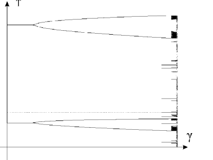
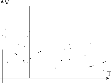
In Fig. 1 transition to chaos is shown. The initial dynamical state with two impacts per period bifurcates at $\gamma=\gamma_{pd}^{\left(2\right)}=0.090099$ (this value can be computed analytically, see [12]). For $\gamma\rightarrow\gamma_{cr}^{\left(2\right)}$ time of the second impact tends to $1$ and this mode of dynamics is impossible for $\gamma>\gamma_{cr}^{\left(2\right)}$. It turns out that for $\gamma>\gamma_{cr}^{\left(2\right)}$ there are two attractors: a noisy, probably chaotic, attractor coexisting with a $7$–cycle which appears just before the transition. At $\gamma=0.09060$ the noisy attractor disappears and is substituted by a more irregular attractor, see Figs. 2,3.

Full circles indicate positions of small clouds of points. We have studied these potentially chaotic attractors in detail. First of all, we have checked numerically that the attractors are non–periodic. Indeed, computations show that after $10^{8}$ iterations the points generated by the map (5), (6) stay on the corresponding attractor and do not repeat. We have also computed Lyapunov exponents for both attractors. In the case of the attractor shown in Fig. 2 the Lyapunov exponent is $\lambda_{1}=0.5$ while for the attractor in Fig. 3 $\lambda_{2}=0.8$. It follows that in both cases dynamics is chaotic and is more mixing in the second case. The mechanism of mixing is explained in the next Section.

Refer to caption
Figure 2: Chaotic attractor, $R=0.85,h=0.2623,\gamma=0.09059$.
Refer to caption
Figure 3: Chaotic attractor, $R=0.85,h=0.2623,\gamma=0.09060$.

4 Mechanism of mixing

Mixing can arise due to corner events [1] when impacts occur at points where motion of the limiter loses smoothness at time instances $T_{cr}^{\left(1\right)}=h$, $T_{cr}^{\left(2\right)}=1$. Let us investigate the second possibility more closely. In Fig. 4 the stable $2^{2}$ - cycle with four impacts per two periods: $0<T_{\ast 1},T_{\ast 3}<h$, $h<T_{\ast 2},T_{\ast 4}<1$ and unstable $2$ - cycle are shown schematically.

Refer to caption

Figure 4: Stable $2^{2}$ - cycle (circles) and the unstable $2$ - cycle (boxes).

For increasing value of the control parameter $\gamma$ we have $T_{\ast 2}\rightarrow T_{cr}^{\left(2\right)}=1$, see Fig. 1. The map (5), (6) is invariant under translation $T_{i}\rightarrow T_{i+1}$ and thus the phase space is topologically equivalent to the cylinder and hence we have to glue the end points of the time interval $\left[0,1\right]$ obtaining thus a circle. Therefore, a small neighborhood of $T_{cr}^{\left(2\right)}=1$ is a union of two sets, $O_{cr}^{\left(2\right)}=\left\{T:\quad 1-\epsilon_{1}<T\leq 1\right\}\cup\left\{T:\quad 0\leq T<\epsilon_{2}\right\}$, where $\epsilon_{1},\ \epsilon_{2}$ are small and positive, see Fig. 5.

Refer to caption
Figure 5: Unstable $2^{2}$ - cycle (circles) and the unstable $2$ - cycle (boxes).

Now, let $T_{i}\in O_{cr}^{\left(2\right)}$. It follows from Eqs. (5), (6) that time of the next impact, $T_{i+1}$, as well as the corresponding post–impact velocity, $V_{i+1}$, depend discontinuously on $T_{i}$. In other words, we get different solutions, $T_{i+1},\,V_{i+1}$, depending on whether $1-\epsilon_{1}<T_{i}<1$ or $0<T_{i}<\epsilon_{2}$. It follows that mixing will necessarily be present if a trajectory recurrently visits the interval $O_{cr}^{\left(2\right)}$. We shall study this possibility in the next Section.

5 Origin of the homoclinic structure

Let us consider critical case: $\gamma=\gamma_{cr}^{\left(1\right)}$, $T_{\ast 2}=T_{cr}^{\left(2\right)}=1$. This is described by Eq. (7) with four impacts per two periods such that $0<T_{\ast 1},T_{\ast 3}<h$, $T_{\ast 2}=1,T_{\ast 4}<1$:

$$\left\{\begin{array}[]{l}0=\frac{\gamma}{h}T_{1}-\left(1-T_{1}\right)^{2}+\left(1-T_{1}\right)V_{1}\\ V_{2}=-RV_{1}+2R\left(1-T_{1}\right)-\frac{\gamma\left(1+R\right)}{1-h}\\ \frac{\gamma}{h}=-\left(T_{3}-1\right)+V_{2}\\ V_{3}=-RV_{2}+2R\left(T_{3}-1\right)+\frac{\gamma\left(1+R\right)}{h}\\ \frac{\gamma\left(-T_{4}+1\right)}{1-h}=\frac{\gamma T_{3}}{h}-\left(T_{4}-T_{3}\right)^{2}+\left(T_{4}-T_{3}\right)V_{3}\\ V_{4}=-RV_{3}+2R\left(T_{4}-T_{3}\right)+\frac{\gamma\left(1+R\right)}{1-h}\\ \frac{\gamma T_{1}}{h}=-\frac{\gamma T_{1}}{1-h}-\left(T_{1}+1-T_{4}\right)^{2}+\left(T_{1}+1-T_{4}\right)V_{4}\\ V_{1}=-RV_{4}+2R\left(T_{1}+1-T_{4}\right)+\frac{\gamma\left(1+R\right)}{h}\end{array}\right.$$ (8)

where we have substituted $T_{2}=1$ and the periodicity conditions: $T_{5}=T_{1}+1$, $V_{5}=V_{1}$. Solutions of Eq. (8) depend on roots of the following algebraic equation:

$$A_{6}X^{6}+A_{5}X^{5}+A_{4}X^{4}+A_{3}X^{3}+A_{2}X^{2}+A_{1}X+A_{0}=0,$$ (9)

where $X\equiv T_{1}$ with coefficients $A_{i}$ depending on $R$, $h$ in a complicated way. The coefficients are listed below:

$$A_{6}=\left(R+1\right)^{2}\left(R^{2}+1\right)^{5},$$

$A_{5}=a_{5}+b_{5}h$:

$\displaystyle a_{5}$ $\displaystyle=$ $\displaystyle 2\left(R+1\right)\left(\begin{array}[]{c}R^{11}-11R^{10}-29R^{9}-17R^{8}+16R^{7}-36R^{6}\\ -48R^{5}-36R^{4}+23R^{3}-9R^{2}-11R-3\end{array}\right),$
$\displaystyle b_{5}$ $\displaystyle=$ $\displaystyle-4R\left(R^{3}-R-2\right)\left(R+1\right)^{2}\left(R^{2}+1\right)^{3},$

$A_{4}=a_{4}+b_{4}h+c_{4}h^{2}$:

$\displaystyle a_{4}$ $\displaystyle=$ $\displaystyle 23+74R-6R^{2}-158R^{3}+121R^{4}+348R^{5}+316R^{6}$
$\displaystyle+28R^{7}+73R^{8}+250R^{9}+170R^{10}+34R^{11}+7R^{12},$
$\displaystyle b_{4}$ $\displaystyle=$ $\displaystyle 4\left(R+1\right)\left(\begin{array}[]{c}17R^{10}+11R^{9}-20R^{8}-49R^{7}+5R^{6}\\ -19R^{5}-41R^{4}-55R^{3}+10R^{2}-3\end{array}\right),$
$\displaystyle c_{4}$ $\displaystyle=$ $\displaystyle 4\left(R^{4}+1\right)\left(R+1\right)^{2}\left(R^{2}+1\right)^{3},$

$A_{3}=a_{3}+b_{3}h+c_{3}h^{2}$:

$\displaystyle a_{3}$ $\displaystyle=$ $\displaystyle 4\left(R+1\right)\left(\begin{array}[]{c}R^{11}-11R^{10}-41R^{9}-55R^{8}+28R^{7}-32R^{6}\\ -48R^{5}-32R^{4}+3R^{3}+43R^{2}-7R-9\end{array}\right),$
$\displaystyle b_{3}$ $\displaystyle=$ $\displaystyle 16-72R-160R^{2}+352R^{3}+520R^{4}+336R^{5}+32R^{6}$
$\displaystyle+416R^{7}+512R^{8}+184R^{9}-128R^{10}-64R^{11}-24R^{12},$
$\displaystyle c_{3}$ $\displaystyle=$ $\displaystyle-8R\left(R+1\right)\left(R^{4}+1\right)\left(R^{6}+9R^{5}+2R^{4}-R^{2}+15R-2\right),$

$A_{2}=a_{2}+b_{2}h+c_{2}h^{2}+d_{2}h^{3}$:

$\displaystyle a_{2}$ $\displaystyle=$ $\displaystyle 31-2R-118R^{2}-178R^{3}+9R^{4}+188R^{5}+252R^{6}$
$\displaystyle-180R^{7}+113R^{8}+358R^{9}+154R^{10}+6R^{11}+7R^{12},$
$\displaystyle b_{2}$ $\displaystyle=$ $\displaystyle-8+192R+120R^{2}-168R^{3}-416R^{4}-176R^{5}-192R^{7}$
$\displaystyle-632R^{8}-208R^{9}+72R^{10}+40R^{11}-32R^{12},$
$\displaystyle c_{2}$ $\displaystyle=$ $\displaystyle 8\left(R^{4}+1\right)\left(\begin{array}[]{c}6R^{8}+10R^{7}+11R^{6}-8R^{5}\\ +3R^{4}+14R^{3}+21R^{2}-8R-1\end{array}\right),$
$\displaystyle d_{2}$ $\displaystyle=$ $\displaystyle 16R\left(R-1\right)\left(R+1\right)\left(R^{4}+1\right)^{2},$

$A_{1}=a_{1}+b_{1}h+c_{1}h^{2}+d_{1}h^{3}$:

$\displaystyle a_{1}$ $\displaystyle=$ $\displaystyle-2\left(R+1\right)^{2}\left(\begin{array}[]{c}3R^{10}+4R^{9}-3R^{8}+92R^{7}-132R^{6}\\ +80R^{5}-16R^{4}+28R^{3}-47R^{2}+4R+3\end{array}\right),$
$\displaystyle b_{1}$ $\displaystyle=$ $\displaystyle-32-64R-180R^{2}+56R^{3}+204R^{4}+112R^{5}-280R^{6}$
$\displaystyle+128R^{7}+392R^{8}+80R^{9}-116R^{10}+72R^{11}+12R^{12},$
$\displaystyle c_{1}$ $\displaystyle=$ $\displaystyle 8\left(R^{4}+1\right)\left(R^{8}-12R^{7}+R^{6}+8R^{5}+R^{4}-20R^{3}-R^{2}+6\right),$
$\displaystyle d_{1}$ $\displaystyle=$ $\displaystyle-16\left(R-1\right)\left(R^{3}+R^{2}+R-1\right)\left(R^{4}+1\right)^{2},$

$A_{0}=a_{0}+b_{0}h+c_{0}h^{2}+d_{0}h^{3}$:

$\displaystyle a_{0}$ $\displaystyle=$ $\displaystyle\left(R-1\right)\left(R^{4}+4R^{2}+4R+3\right)\left(\begin{array}[]{c}R^{7}+7R^{6}+9R^{5}-13R^{4}\\ +7R^{3}+9R^{2}-R-3\end{array}\right),$
$\displaystyle b_{0}$ $\displaystyle=$ $\displaystyle-4\left(R-1\right)\left(\begin{array}[]{c}3R^{10}+9R^{9}-12R^{8}+25R^{7}+29R^{6}+15R^{5}\\ -9R^{4}+23R^{3}+24R^{2}+8R-3\end{array}\right),$
$\displaystyle c_{0}$ $\displaystyle=$ $\displaystyle-4\left(R-1\right)\left(R^{4}+1\right)\left(\begin{array}[]{c}R^{7}+3R^{6}-15R^{5}+11R^{4}\\ +3R^{3}-7R^{2}-13R+1\end{array}\right),$
$\displaystyle d_{0}$ $\displaystyle=$ $\displaystyle 16R\left(R-1\right)^{2}\left(R^{4}+1\right)^{2}.$

Let us stress here that acceptable solution for the time of the first impact must fulfill consistency condition $T_{1}\equiv X\in\left(0,h\right)$. Now it follows that necessary conditions for existence of this solution can be formulated. Indeed, the condition $A_{0}=f\left(R,h\right)=0$ guarantees existence of solution $T_{1}\equiv X=0$. Furthermore, after change of variable $X=\tilde{X}+h$ the equation (9) is written as $\tilde{A}_{6}\tilde{X}^{6}+\ldots+\tilde{A}_{1}\tilde{X}+\tilde{A}_{0}=0$ and the condition $\tilde{A}_{0}=A_{6}h^{6}+A_{5}h^{5}+A_{4}h^{4}+A_{3}h^{3}+A_{2}h^{2}+A_{1}h+A_{0}=0$ guarantees existence of the solution $\tilde{X}=0$ and hence existence of solution $T_{1}\equiv X=h$. Region of acceptable values of parameters $R$, $h$ is shown in Fig. 6 - it is placed between thin solid lines (which correspond to the condition $T_{1}=h$) and below medium solid line (the condition $T_{1}=0$).

Refer to caption
Figure 6: Acceptable parameter values (shaded region).

The solution of Eq. (8) is unstable and leads to a homoclinic–type orbit and thus can be referred to as the homoclinic cycle (see [13] for the definition of a homoclinic point and a homoclinic orbit). Indeed, for the initial condition $1-\epsilon_{1}<T_{2}<1$ the orbit is attracted by the $2^{2}$ - cycle $T_{\ast 1},T_{\ast 2}=1,T_{\ast 3},T_{\ast 4}$, while for $0<T_{2}<\epsilon_{2}$ the fixed point $T_{\ast 2}=1$ is repelling, but the orbit returns eventually to the $2^{2}$ - cycle (provided that a coexisting attractor does not capture the trajectory). We shall compute the repelling branch in the next Section.

6 Computing the homoclinic orbit

To analyse structure of the chaotic attractor shown in Fig. 2 we have solved Eq. (8) for $R=0.85$, $h=0.2623$, computing thus critical value of the parameter $\gamma$ and the homoclinic cycle where $\left(T_{\ast 2},V_{\ast 2}\right)$ is the homoclinic point:

$$\begin{array}[]{ll}\gamma_{cr}^{\left(1\right)}=0.090\,581\,947\,119\,,&\\ T_{\ast 1}=0.122\,922\,181\,823\,,&V_{\ast 1}=0.828\,678\,917\,871\,,\\ T_{\ast 2}=1^{-}\,,&V_{\ast 2}=0.559\,494\,302\,251\,,\\ T_{\ast 3}=0.\,214\,157\,103\,932\,,&V_{\ast 3}=0.527\,370\,736\,661\,,\\ T_{\ast 4}=0.827\,577\,663\,824\,,&V_{\ast 4}=0.367\,388\,917\,196\,.\end{array}$$ (18)

This solution is attracting for initial condition $T_{2}\in\left(1-\epsilon_{1},1\right)$ and $V_{2}\cong V_{\ast 2}$. The sequence $\left\{T_{i},V_{i}\right\}$ starting from such initial condition belongs to the attracting branch of the homoclinic orbit. The repelling branch is obtained in the following way. We start from $T_{1}=T_{\ast 1}$, $V_{1}=V_{\ast 1}$. $T_{2}$ and $V_{2}$ are computed from the following equations:

$\displaystyle\frac{\gamma}{h}\left(T_{2}-1\right)$ $\displaystyle=$ $\displaystyle\frac{\gamma}{h}T_{\ast 1}-\left(T_{2}-T_{\ast 1}\right)^{2}+\left(T_{2}-T_{\ast 1}\right)V_{\ast 1}$ (19)
$\displaystyle V_{2}$ $\displaystyle=$ $\displaystyle-RV_{\ast 1}+2R\left(T_{2}-T_{\ast 1}\right)+\left(1+R\right)\frac{\gamma}{h}$ (20)

The solution of the first equation is of course $T_{2}=1$. We assume now in (20) that at the impact the table is just about going up with velocity $\dot{Y}\left(T_{2}\right)=1/h$ rather than it has just finished going down with velocity $\dot{Y}\left(T_{2}\right)=-1/\left(1-h\right)$ (therefore this equation differs from the second of equations in (8)). We thus compute from Eq. (20), for $R=0.85$, $h=0.2623$ and $\gamma=\gamma_{cr}^{\left(1\right)}=0.090\,581\,947\,119$, that $V_{2}=1.\,425\,529\,027\,600$ (let us stress again that using the second of Eqs. (8) we get $V_{\ast 2}=0.559\,494\,302\,251$) . Due to symmetry of the dynamics $T_{i}\rightarrow T_{i}+1$ the first point of the repelling branch of the homoclinic orbit can be assumed as $T_{1}^{R}=0$, $V_{1}^{R}=1.\,425\,529\,027\,600$ .

We have thus computed numerically the repelling branch of the homoclinic orbit starting from the initial condition $T_{1}^{R}$, $V_{1}^{R}$ ($R=0.85$, $h=0.2623$, $\gamma=\gamma_{cr}^{\left(1\right)}=0.090\,581\,947\,119$).

Refer to caption
Figure 7: The homoclinic orbit.

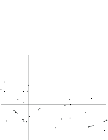
We have shown in Fig. 6 first twenty six points (full circles) of the repelling branch of the homoclinic orbit starting from the point $\left(T_{1}^{R},V_{1}^{R}\right)$ - the outermost full circle in the figure, lying on the vertical axis. These points agree very well with positions of twenty six clouds of points belonging to the chaotic attractor shown in Fig. 2, computed for $\gamma=0.09059$. The next points (dots) of the repelling branch of the homoclinic trajectory enter four connected parts placed as in Fig. 2 and tend, as an attracting branch, to the homoclinic cycle (larger open circles) containing the homoclinic point $\left(T_{\ast 2},V_{\ast 2}\right)$ - the outermost open circle.

This homoclinic structure is preserved in the interval $\gamma_{cr}^{\left(1\right)}=0.0905819471\ldots<\gamma<0.09060$, $R=0.85$, $h=0.2623$ until this attractor is substituted by a new one due to crisis (the unstable cycle collides with one of clouds of points belonging to the attractor), see the bifurcation diagram, Fig. 1, and Figs. 2,3.

7 Summary and discussion

We have found a generic scenario of transition to chaos for dynamics of a ball moving vertically in gravitational field and colliding with a table moving vertically with piecewise constant velocity.

According to this scenario a periodic and stable solution is destroyed via a corner bifurcation [1] in a corner event, $T_{\ast i}=T_{cr}^{\left(1\right)}=h$ or $T_{\ast i}=T_{cr}^{\left(2\right)}=1$. In the present paper the solution, defined analytically by $T_{\ast 2}=1$ in Eq. (7), is a homoclinic–type orbit and leads to mixing and hence to chaotic dynamics. This homoclinic–type orbit is untypical in the sense that it is not a saddle structure but its origin is related to discontinuous dynamics in the neighborhood of $T_{cr}^{\left(2\right)}$.

References

  • [1] M. di Bernardo, C.J. Budd, A.R. Champneys, P. Kowalczyk, Piecewise-Smooth Dynamical Systems. Theory and Applications. Series: Applied Mathematical Sciences, vol. 163. Springer, Berlin (2008).
  • [2] A.C.J.Luo, Singularity and Dynamics on Discontinuous Vector Fields. Monograph Series on Nonlinear Science and Complexity, vol. 3. Elsevier, Amsterdam (2006).
  • [3] J. Awrejcewicz, C.-H. Lamarque, Bifurcation and Chaos in NonsmoothMechanical Systems.World Scientific Series on Nonlinear Science: Series A, vol. 45. World Scientific Publishing, Singapore (2003).
  • [4] A.F. Filippov, Differential Equations with Discontinuous Right-Hand Sides. Kluwer Academic, Dordrecht (1988).
  • [5] W.J. Stronge, Impact mechanics. Cambridge University Press, Cambridge (2000).
  • [6] A. Mehta (ed.), Granular Matter: An Interdisciplinary Approach. Springer, Berlin (1994).
  • [7] C. Knudsen, R. Feldberg, H. True, Bifurcations and chaos in a model of a rolling wheel-set. Philos. Trans. R. Soc. Lond. A 338 (1992) 455–469.
  • [8] M. Wiercigroch, A.M. Krivtsov, J. Wojewoda, Vibrational energy transfer via modulated impacts for percussive drilling. Journal of Theoretical and Applied Mechanics 46 (2008) 715-726.
  • [9] A. C. J. Luo, Y. Guo, Motion Switching and Chaos of a Particle in a Generalized Fermi-Acceleration Oscillator, Mathematical Problems in Engineering, vol. 2009, Article ID 298906, 40 pages, 2009. doi:10.1155/2009/298906.
  • [10] A. Okninski, B. Radziszewski, Chaotic dynamics in a simple bouncing ball model, Proceedings of the 10th Conference on Dynamical Systems: Theory and Applications, December 7-10, 2009. Łódź, Poland, J. Awrejcewicz, M. Kazmierczak, P. Olejnik, J. Mrozowski (eds.), pp. 651-656.
  • [11] A. Okninski, B. Radziszewski, Grazing dynamics and dependence on initial conditions in certain systems with impacts, arXiv:0706.0257 (2007).
  • [12] A. Okninski, B. Radziszewski, Dynamics of impacts with a table moving with piecewise constant velocity, Nonlinear Dynamics 58 (2009) 515-523.
  • [13] Robert L. Devaney, An Introduction to Chaotic Dynamical Systems. Westview Press (2003).