Multiple trains of same-color surface plasmon-polaritons guided by the planar interface of a metal and a sculptured nematic thin film.
Part IV: Canonical problem

Muhammad Faryad,^a John A. Polo Jr.,^b and Akhlesh Lakhtakia^a,c

^aNanoengineered Metamaterials Group (NanoMM), Department of Engineering Science and Mechanics, Pennsylvania State University, University Park, PA 16802-6812, USA

^bDepartment of Physics and Technology, Edinboro University of Pennsylvania, 235 Scotland Rd., Edinboro, PA 16444, USA

^cDepartment of Physics, Indian Institute of Technology Kanpur, Kanpur (UP) 208016, India

Abstract. The canonical problem of the propagation of surface-plasmon-polariton (SPP) waves localized to the planar interface of a metal and a sculptured nematic thin film (SNTF) that is periodically nonhomogeneous along the direction normal to the interface was formulated. Solution of the dispersion equation obtained thereby confirmed the possibility of exciting multiple SPP waves of the same frequency or color. However, these SPP waves differ in phase speed, field structure, and the e-folding distance along the direction of propagation.

1 Introduction

Among the various forms of electromagnetic surface waves, the surface-plasmon-polariton (SPP) wave has the longest history of theoretical development and application. Arising from earlier developments, the SPP wave was envisioned in the mid-twentieth century as a wave guided by the planar interface of a metal and an isotropic dielectric material. Since that time, the theory has evolved to encompass interfaces between a metal and various dielectric materials of greater complexity. The inclusion of anisotropic, homogeneous dielectrics[1, 2, 3, 4, 5, 6, 7, 8] in the study of electromagnetic surface waves has been considered for some time now. More recently, SPP waves at the interface of a metal and a nonhomogeneous dielectric material, which exhibit several interesting properties, has been receiving considerable attention. The nonhomogeneous dielectric materials investigated include continuously varying materials[11, 12, 9, 10] such as liquid crystals, as well as layered structures[13, 14, 15, 16].

This series of papers is devoted to theoretical and experimental investigations on the propagation of a surface electromagnetic wave guided by the planar interface of a metal and a sculptured nematic thin film (SNTF), the latter being periodically nonhomogeneous in the direction normal to the interface. In Parts I [17] and II [18], the absorbance, reflectance and transmittance of an incident linearly polarized plane wave were calculated when this planar interface is implemented via a metal-SNTF bilayer and a prism in a Kretschmann setup. The wavevector of the incident plane wave was supposed to lie wholly in the morphologically significant plane of the SNTF, but that restriction was lifted in Part II. The computed results showed that multiple surface-plasmon-polariton (SPP) waves, all of the same frequency or color, can be excited at the metal/SNTF interface. The guided SPP waves possess different field structures as well as different phase speeds.

In Part III [19], experimentally obtained data was presented in support of the theoretical predictions of Part I. The absorbances of two different metal-SNTF bilayers were evaluated as the difference between unity and the measured reflectance, the transmittance being assumed to be null-valued at angles of incidence exceeding the critical angle for the interface of the SNTF with the prism. Analysis of the collected data confirmed the possibility of exciting multiple SPP waves with different phase speeds and field structures. Parenthetically, in a parallel effort the same possibility was theoretically predicted [9, 10] and validated experimentally [20] for the planar interface of a metal and a chiral sculptured thin film [21, 22].

The method adopted for theoretical predictions and experimental verification in Parts I–III was an indirect one, because the existence of SPP waves was deduced from the absorbance, reflectance and transmittance characteristics of a metal-SNTF bilayer. Each layer in the bilayer is of finite thickness. In the canonical problem of SPP-wave propagation, the metal and the SNTF have to be semi-infinite. The solution of the canonical problem provides incontrovertible proof of the existence of multiple SPP-wave modes, and also eliminates possible confusion with waveguide modes spread over the entirety of the SNTF. Accordingly, for this paper, we set out to prove the existence of multiple SPP waves directly. The approach adopted by us is similar to that of Agarwal et al. [23], being independent of any incident plane wave. The formulated boundary-value problem was solved numerically for the SPP wavenumbers.

The canonical problem is formulated in Sec. 2, and numerical results are presented and discussed in Sec. 3. An $\exp(-i\omega t)$ time-dependence is implicit, with $\omega$ denoting the angular frequency. The free-space wavenumber, the free-space wavelength, and the intrinsic impedance of free space are denoted by $k_{\scriptscriptstyle 0}=\omega\sqrt{\epsilon_{\scriptscriptstyle 0}\mu_{\scriptscriptstyle 0}}$, $\lambda_{\scriptscriptstyle 0}=2\pi/k_{\scriptscriptstyle 0}$, and $\eta_{\scriptscriptstyle 0}=\sqrt{\mu_{\scriptscriptstyle 0}/\epsilon_{\scriptscriptstyle 0}}$, respectively, with $\mu_{\scriptscriptstyle 0}$ and $\epsilon_{\scriptscriptstyle 0}$ being the permeability and permittivity of free space. Vectors are in boldface, dyadics are underlined twice, column vectors are in boldface and enclosed within square brackets, and matrixes are underlined twice and square-bracketed. The asterisk denotes the complex conjugate, and the Cartesian unit vectors are identified as $\hat{{\bf u}}_{x}$, $\hat{{\bf u}}_{y}$, and $\hat{{\bf u}}_{z}$.

2 Theory

Let the half-space $z\leq 0$ be occupied by an isotropic and homogeneous metal with complex-valued relative permittivity scalar $\epsilon_{met}$. The region $z\geq 0$ is occupied by the chosen SNTF with a periodically nonhomogeneous permittivity dyadic [17, 18, 19]

$$\underline{\underline{\epsilon}}_{SNTF}(z)=\epsilon_{\scriptscriptstyle 0}\,\underline{\underline{S}}_{y}(z)\cdot\underline{\underline{\epsilon}}^{\circ}_{ref}(z)\cdot\underline{\underline{S}}_{y}^{-1}(z)\,,$$ (1)

where the dyadics

$$\left.\begin{array}[]{l}\underline{\underline{S}}_{y}(z)=(\hat{{\bf u}}_{x}\hat{{\bf u}}_{x}+\hat{{\bf u}}_{z}\hat{{\bf u}}_{z})\cos\left[\chi(z)\right]+(\hat{{\bf u}}_{z}\hat{{\bf u}}_{x}-\hat{{\bf u}}_{x}\hat{{\bf u}}_{z})\sin\left[\chi(z)\right]+\hat{{\bf u}}_{y}\hat{{\bf u}}_{y}\\[5.0pt] \underline{\underline{\epsilon}}^{\circ}_{ref}(z)=\epsilon_{a}(z)\,\hat{{\bf u}}_{z}\hat{{\bf u}}_{z}+\epsilon_{b}(z)\,\hat{{\bf u}}_{x}\hat{{\bf u}}_{x}+\epsilon_{c}(z)\,\hat{{\bf u}}_{y}\hat{{\bf u}}_{y}\end{array}\right\}$$ (2)

depend on the vapor incidence angle $\chi_{v}(z)={\tilde{\chi}}_{v}+\delta_{v}\,\sin(\pi z/\Omega)$ that varies sinusoidally with period $2\Omega$.

In order to investigate SPP-wave propagation, we adopted a procedure devised to investigate the propagation of Dyakonov–Tamm waves [23]. Let the SPP wave propagate parallel to the unit vector $\hat{{\bf u}}_{x}\cos\psi+\hat{{\bf u}}_{y}\sin\psi$ along the interface $z=0$, and attenuate as $z\to\pm\infty$. Therefore, in the region $z\leq 0$, the wave vector may be written as

$${\bf k}_{met}=\kappa\,\hat{{\bf u}}_{1}-\alpha_{met}\,\hat{{\bf u}}_{z}\,,$$ (3)

where $\kappa^{2}+\alpha_{met}^{2}=k_{\scriptscriptstyle 0}^{2}\,\epsilon_{met}$, $\kappa$ is complex-valued, and ${\rm Im}(\alpha_{met})>0$ for attenuation as $z\to-\infty$; here and hereafter, the unit vectors $\hat{{\bf u}}_{1}=\hat{{\bf u}}_{x}\cos\psi+\hat{{\bf u}}_{y}\sin\psi$ and $\hat{{\bf u}}_{2}=-\hat{{\bf u}}_{x}\sin\psi+\hat{{\bf u}}_{y}\cos\psi$. Accordingly, the field phasors in the metal may be written as

$${\bf E}({\bf r})=\left[a_{p}\left(\frac{\alpha_{met}}{k_{\scriptscriptstyle 0}}\,\hat{{\bf u}}_{1}+\frac{\kappa}{k_{\scriptscriptstyle 0}}\,\hat{{\bf u}}_{z}\right)+a_{s}\,\hat{{\bf u}}_{2}\right]\exp(i{\bf k}_{met}\cdot{\bf r})\,,\quad z\leq 0\,,$$ (4)

and

$${\bf H}({\bf r})=\eta_{\scriptscriptstyle 0}^{-1}\left[-a_{p}\,\epsilon_{met}\,\hat{{\bf u}}_{2}+a_{s}\left(\frac{\alpha_{met}}{k_{\scriptscriptstyle 0}}\,\hat{{\bf u}}_{1}+\frac{\kappa}{k_{\scriptscriptstyle 0}}\,\hat{{\bf u}}_{z}\right)\right]\exp(i{\bf k}_{met}\cdot{\bf r})\,,\quad z\leq 0\,,$$ (5)

where $a_{p}$ and $a_{s}$ are unknown scalars.

For field representation in the SNTF, let us write ${\bf E}({\bf r})={\bf e}(z)\,\exp\left({i\kappa\hat{{\bf u}}_{1}\cdot{\bf r}}\right)$ and ${\bf H}({\bf r})={\bf h}(z)\,\exp\left({i\kappa\hat{{\bf u}}_{1}\cdot{\bf r}}\right)$. The components $e_{z}(z)$ and $h_{z}(z)$ of the field phasors can be found in terms of the other components as follows:

$$e_{z}(z) = \frac{\epsilon_{d}(z)\left[\epsilon_{a}(z)-\epsilon_{b}(z)\right]\sin\left[\chi(z)\right]\cos\left[\chi(z)\right]}{\epsilon_{a}(z)\epsilon_{b}(z)}e_{x}(z)$$ (6)

$$+\kappa\frac{\epsilon_{d}(z)}{\omega\epsilon_{\scriptscriptstyle 0}\epsilon_{a}(z)\epsilon_{b}(z)}\left[h_{x}(z)\sin\psi-h_{y}(z)\cos\psi\right],\quad z>0\,,$$

$$h_{z}(z) = -\,\frac{\kappa}{\omega\mu_{\scriptscriptstyle 0}}\left[e_{x}(z)\sin\psi-e_{y}(z)\cos\psi\right],\quad z>0\,,$$ (7)

where

$$\epsilon_{d}(z)=\frac{\epsilon_{a}(z)\,\epsilon_{b}(z)}{\epsilon_{a}(z)\,\cos^{2}\left[\chi(z)\right]+\epsilon_{b}(z)\,\sin^{2}\left[\chi(z)\right]}\,.$$ (8)

The other components of the electric and magnetic field phasors are used in the column vector

$$\left[{\bf f}(z)\right]=\left[e_{x}(z)\quad e_{y}(z)\quad h_{x}(z)\quad h_{y}(z)\right]^{T}\,$$ (9)

which satisfies the matrix differential equation [23]

$$\frac{d}{dz}\left[{\bf f}(z)\right]=i\left[\underline{\underline{P}}(z)\right]\cdot\left[{\bf f}(z)\right]\,,\quad z>0\,,$$ (10)

where the 4$\times$4 matrix

$$[\underline{\underline{P}}(z)]=\omega\,\left[\begin{array}[]{cccc}0&0&0&\mu_{\scriptscriptstyle 0}\\ 0&0&-\mu_{\scriptscriptstyle 0}&0\\ 0&-\epsilon_{\scriptscriptstyle 0}\,\epsilon_{c}(z)&0&0\\ \epsilon_{\scriptscriptstyle 0}\,\epsilon_{d}(z)&0&0&0\end{array}\right]$$ (15)

$$\qquad+\,\kappa\,\frac{\epsilon_{d}(z)\,\left[\epsilon_{a}(z)-\epsilon_{b}(z)\right]}{\epsilon_{a}(z)\,\epsilon_{b}(z)}\,\sin\left[\chi(z)\right]\,\cos\left[\chi(z)\right]\,\left[\begin{array}[]{cccc}\cos\psi&0&0&0\\ \sin\psi&0&0&0\\ 0&0&0&0\\ 0&0&-\sin\psi&\cos\psi\end{array}\right]$$ (20)

$$\qquad\quad+\,\frac{\kappa^{2}}{\omega\epsilon_{\scriptscriptstyle 0}}\,\frac{\epsilon_{d}(z)}{\epsilon_{a}(z)\,\epsilon_{b}(z)}\,\left[\begin{array}[]{cccc}0&0&\cos\psi\,\sin\psi&-\cos^{2}\psi\\ 0&0&\sin^{2}\psi&-\cos\psi\,\sin\psi\\ 0&0&0&0\\ 0&0&0&0\end{array}\right]$$ (25)

$$\qquad\qquad+\,\frac{\kappa^{2}}{\omega\mu_{\scriptscriptstyle 0}}\,\left[\begin{array}[]{cccc}0&0&0&0\\ 0&0&0&0\\ -\cos\psi\,\sin\psi&\cos^{2}\psi&0&0\\ -\sin^{2}\psi&\cos\psi\,\sin\psi&0&0\end{array}\right]\,.$$ (30)

As in Part II, we used the piecewise uniform approximation technique [22] to determine the matrix $[\underline{\underline{Q}}]$ that appears in the relation

$$[{\bf f}(2\Omega)]=[\underline{\underline{Q}}]\cdot[{\bf f}(0+)]$$ (31)

to characterize the optical response of one period of the chosen SNTF for specific values of $\kappa$ and $\psi$. By virtue of the Floquet–Lyapunov theorem [24], a matrix $[\underline{\underline{{\tilde{Q}}}}]$ can be defined such that

$$[\underline{\underline{Q}}]=\exp\left\{i2\Omega[\underline{\underline{{\tilde{Q}}}}]\right\}\,.$$ (32)

Both $[\underline{\underline{Q}}]$ and $[\underline{\underline{{\tilde{Q}}}}]$ share the same eigenvectors, and their eigenvalues are also related. Let $[{\bf t}]^{(n)}$, $n\in\left[1,4\right]$, be the eigenvector corresponding to the $n$th eigenvalue $\sigma_{n}$ of $[\underline{\underline{Q}}]$; then, the corresponding eigenvalue $\alpha_{n}$ of $[\underline{\underline{{\tilde{Q}}}}]$ is given by

$$\alpha_{n}=-i\frac{\ln\sigma_{n}}{2\Omega}\,,\qquad n\in\left[1,4\right]\,.$$ (33)

After ensuring that ${\rm Im}({\alpha_{1,2}})>0$, we set

$$[{\bf f}(0+)]=\left[\,[{\bf t}]^{(1)}\quad[{\bf t}]^{(2)}\,\right]\cdot\left[\begin{array}[]{c}b_{1}\\ b_{2}\end{array}\right]\,$$ (34)

for SPP-wave propagation, where $b_{1}$ and $b_{2}$ are unknown scalars; the other two eigenvalues of $[\underline{\underline{{\tilde{Q}}}}]$ pertain to waves that amplify as $z\to\infty$ and cannot therefore contribute to the SPP wave. At the same time,

$$[{\bf f}(0-)]=\left[\begin{array}[]{cc}\frac{\alpha_{met}}{k_{\scriptscriptstyle 0}}\,\cos\psi&-\sin\psi\\[5.0pt] \frac{\alpha_{met}}{k_{\scriptscriptstyle 0}}\,\sin\psi&\cos\psi\\[5.0pt] \frac{\epsilon_{met}}{\eta_{\scriptscriptstyle 0}}\,\sin\psi&\frac{\alpha_{met}}{k_{\scriptscriptstyle 0}\eta_{\scriptscriptstyle 0}}\,\cos\psi\\[5.0pt] -\frac{\epsilon_{met}}{\eta_{\scriptscriptstyle 0}}\,\cos\psi&\frac{\alpha_{met}}{k_{\scriptscriptstyle 0}\eta_{\scriptscriptstyle 0}}\,\sin\psi\end{array}\right]\cdot\left[\begin{array}[]{c}a_{p}\\ a_{s}\end{array}\right]\,,$$ (35)

by virtue of (4) and (5). Continuity of the tangential components of the electric and magnetic field phasors across the plane $z=0$ requires that $[{\bf f}(0-)]=[{\bf f}(0+)]$, which may be rearranged as the matrix equation

$$[\underline{\underline{Y}}]\cdot\left[\begin{array}[]{c}a_{p}\\ a_{s}\\ b_{1}\\ b_{2}\end{array}\right]=\left[\begin{array}[]{c}0\\ 0\\ 0\\ 0\end{array}\right]\,.$$ (36)

For a nontrivial solution, the 4$\times$4 matrix $[\underline{\underline{Y}}]$ must be singular, so that

$${\rm det}\,[\underline{\underline{Y}}]=0$$ (37)

is the dispersion equation for the SPP wave. This equation has to be solved in order to determine the SPP wavenumber $\kappa$.

3 Numerical Results and Discussion

A Mathematica™ program was written and implemented to solve (37) using the Newton–Raphson method [26] to obtain $\kappa$ for a specific value of $\psi$. The free-space wavelength was fixed at $\lambda_{\scriptscriptstyle 0}=633$ nm. The metal was taken to be aluminum: $\epsilon_{met}=-56+21i$. The SNTF was chosen to be made of titanium oxide [25], with

$$\left.\begin{array}[]{l}\epsilon_{a}(z)=[1.0443+2.7394v(z)-1.3697v^{2}(z)]^{2}\\[5.0pt] \epsilon_{b}(z)=[1.6765+1.5649v(z)-0.7825v^{2}(z)]^{2}\\[5.0pt] \epsilon_{c}(z)=[1.3586+2.1109v(z)-1.0554v^{2}(z)]^{2}\\[5.0pt] \chi(z)=\tan^{-1}[2.8818\tan\chi_{v}(z)]\end{array}\right\}$$ (38)

where $v(z)=2\chi_{v}(z)/\pi$. The angles $\tilde{\chi}_{v}$ and $\delta_{v}$ were taken to be 45^∘ and 30^∘, respectively, and $\Omega=200$ nm for all results presented here.

$\begin{array}[]{cc}\includegraphics[width=126.47249pt]{Faryad_09_1Fig1a.eps}&\includegraphics[width=126.47249pt]{Faryad_09_1Fig1b.eps}\end{array}$

Figure 1: (left) Real and (right) imaginary parts of $\kappa$ as functions of $\psi$, for SPP-wave propagation guided by the planar interface of aluminum and a titanium-oxide SNTF. See the text for the constitutive parameters used. Either two or three modes are possible, depending on $\psi$.

The wavenumber $\kappa$ must be complex-valued for the canonical problem but only real-valued for the Kretschmann configuration [9]. Computed values of the real and imaginary parts of $\kappa$ for the canonical problem are shown in Fig. 1. For $0^{\circ}\leq\psi\lesssim 36^{\circ}$, we found three values of $\kappa$ which satisfy (37) and therefore represent SPP waves. For $36^{\circ}\lesssim\psi\leq 90^{\circ}$, there are two values of $\kappa$ which satisfy (37). This trend is fully consistent with the conclusions drawn in Part II for the Kretschmann configuration. The different solutions of (37) for any specific value of $\psi$ indicate that the SPP waves have different phase speeds $\omega/{\rm Re}(\kappa)$—as theoretically predicted in Parts I and II, and experimentally confirmed in Part III—and different e-folding distances $1/{\rm Im}(\kappa)$ along the direction of propagation.

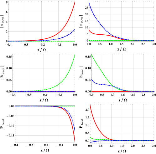
Figure 2: Variations of components of ${\bf e}$, ${\bf h}$, and ${\bf P}$ with $z$, for $\kappa=(2.455+i0.04208)k_{\scriptscriptstyle 0}$ and $\psi=0^{\circ}$. The $x$-, $y$-, and $z$-directed components are represented by solid, dashed and chain-dashed lines, respectively. The data were computed by setting $a_{p}=1$ V m^-1, with $a_{p}$, $b_{1}$, and $b_{2}$ then obtained using (36).

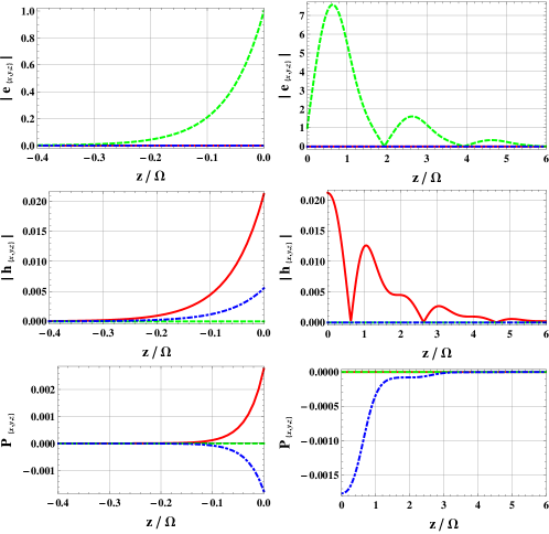
Figure 3: Same as Fig. 2 except for $\kappa=(2.080+i0.003538)k_{\scriptscriptstyle 0}$. The data were computed by setting $a_{s}=1$ V m^-1, with $a_{s}$, $b_{1}$, and $b_{2}$ then obtained using (36).

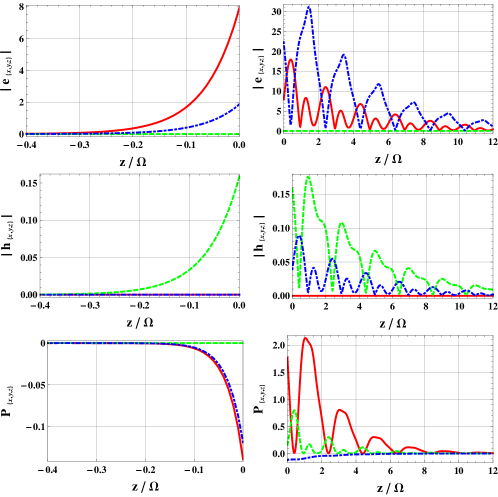
Figure 4: Same as Fig. 2 except for $\kappa=(1.868+i0.007267)k_{\scriptscriptstyle 0}$.

Specifically, for $\psi=0^{\circ}$ the values of $\kappa$ which satisfy (37) are $\kappa_{1}=(2.455+i0.04208)k_{\scriptscriptstyle 0}$, $\kappa_{2}=(2.080+i0.003538)k_{\scriptscriptstyle 0}$, and $\kappa_{3}=(1.868+i0.007267)k_{\scriptscriptstyle 0}$. These solutions represent SPP waves with wave vectors lying wholly in the morphologically significant plane of the SNTF, as addressed theoretically in Part I and experimentally in Part III.

The Cartesian components of the electric and magnetic field phasors and the time-averaged Poynting vector $\bf{P}={1\over 2}{\rm Re}\left(\bf{E}\times\bf{H}^{\ast}\right)$ as functions of $z$ along the line ($x=0$, $y=0$) are shown for $\kappa_{1}$ in Fig. 2, and for $\kappa_{3}$ in Fig. 4. These SPP waves are $p$-polarized, and were respectively labeled as $p1$ and $p2$ in Part III. Figure 3 shows the variations of ${\bf e}$, ${\bf h}$, and ${\bf P}$ along the $z$ axis for $\kappa=\kappa_{2}$. This SPP wave is $s$-polarized and was labeled as $s3$ in Part III. The localization of all three SPP waves around the interface $z=0$ is evident from Figs. 2–4. Also, the SPP wave $p1$ is more localized inside the SNTF than either $p2$ or $s3$. Furthermore, the phase speed of $p1$ is higher than that of $s3$, which exceeds the phase speed of $p2$. However, $s3$ will travel a longer distance along the interface than either $p1$ or $p2$, which could not have been deduced from the theoretical analysis for the Kretschmann configuration in Part I.

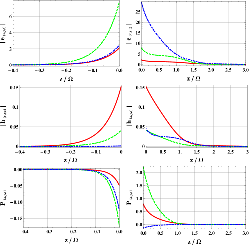
Figure 5: Same as Fig. 2 except for $\kappa=(2.459+i0.04247)k_{\scriptscriptstyle 0}$ and $\psi=75^{\circ}$.

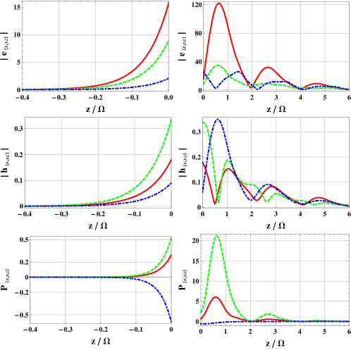
Figure 6: Same as Fig. 2 except for $\kappa=(2.066+i0.003861)k_{\scriptscriptstyle 0}$ and $\psi=75^{\circ}$.

For $\psi=75^{\circ}$, only two values of $\kappa$ were found to satisfy (37): $\kappa_{1}=(2.459+i0.04247)k_{\scriptscriptstyle 0}$ and $\kappa_{2}=(2.066+i0.003861)k_{\scriptscriptstyle 0}$. The variations of ${\bf e}$, ${\bf h}$, and ${\bf P}$ along the $z$ axis are shown in Fig. 5 for $\kappa_{1}$, and in Fig. 6 for $\kappa_{2}$. These two SPP waves cannot be classified as either $p$- or $s$-polarized, which is consistent with the deductions in Part II for the Kretschmann configuration. Although the phase speed of the SPP wave with $\kappa=\kappa_{1}$ exceeds the phase speed of the other SPP wave ($\kappa=\kappa_{2}$), the latter SPP wave will propagate a longer distance along the interface than the former SPP wave.

4 Concluding Remarks

In Parts I and II of this series, the possibility of excitation of multiple SPP waves guided by the planar interface of a metal and a periodically nonhomogeneous SNTF was predicted after solving a boundary-value problem that models the Kretschmann setup. In Part III, an experimental validation was provided for the results of Part I. However, these approaches were indirect and a direct proof of the existence of multiple SPP waves was lacking.

The direct proof was provided here after formulating and solving the canonical problem of propagation guided by the planar interface of semi-infinite expanses of the metal and the periodically nonhomogeneous SNTF. Not only were the conclusions obtained in Parts I–III upheld, but additional information on the e-folding distance along the direction of propagation also emerged from the solution of the canonical problem.

Acknowledgments. MF thanks the Trustees of the Pennsylvania State University for a University Graduate Fellowship. AL is grateful to Charles Godfrey Binder Endowment at the Pennsylvania State University for partial support of this work.

Muhammad Faryad received a B.Sc. degree in Mathematics and Physics from University of Punjab, Lahore, Pakistan, in 2002, and M.Sc. and M.Phil. degrees in Electronics from Quaid-i-Azam University, Islamabad, Pakistan in 2006 and 2008, respectively. His research experience includes analysis of high-frequency fields reflected from cylindrical reflectors in an isotropic chiral medium and the fractional curl operator in electromagnetics. Currently, he is a doctoral student at the Pennsylvania State University. He is a student member of SPIE.

John A. Polo Jr. received a B.S. degree in Physics from the University of Massachusetts, Amherst in 1973 and a Ph.D. degree in Physics from the University of Virginia in 1979. He has held his present position at Edinboro University of Pennsylvania since 1990. His research in the past was conducted in experimental condensed matter physics. Since 2000 he has been working in electromagnetics theory with current research interests in the optical properties of complex materials and metamaterials. He is a member of SPIE.

Akhlesh Lakhtakia received degrees from the Banaras Hindu University (B.Tech. & D.Sc.) and the University of Utah (M.S. & Ph.D.), in Electronics Engineering and Electrical Engineering, respectively. He is the Charles Godfrey Binder (Endowed) Professor of Engineering Science and Mechanics at the Pennsylvania State University. His current research interests include nanotechnology, plasmonics, complex materials, metamaterials, and sculptured thin films. He is a Fellow of SPIE, OSA, AAAS, and the Institute of Physics (UK).

References

- [1] G. Borstel and H. J. Falge, “Surface phonon-polaritons,” in Electromagnetic Surface Modes, A. D. Boardman, Ed., Chap. 6, Wiley, New York, NY, USA (1982).
- [2] R. F. Wallis, “Surface magnetoplasmons on semiconductors,” in Electromagnetic Surface Modes, A. D. Boardman, Ed., Chap. 15, Wiley, New York, NY, USA (1982).
- [3] S. J. Elston and J. R. Sambles, “Surface plasmon-polaritons on an anisotropic substrate,” J. Mod. Opt. 37, 1895-1902 (1990) [doi:10.1080/09500349014552101].
- [4] R. A. Depine and M. L. Gigli, “Excitation of surface plasmons and total absorption of light at the flat boundary between a metal and a uniaxial crystal,” Opt. Lett. 20, 2243-2245 (1995) [doi:10.1364/OL.20.002243].
- [5] H. Wang, “Excitation of surface plasmon oscillations at an interface between anisotropic dielectric and metallic media,” Opt. Mater. 4, 651-656 (1995) [doi:10.1016/0925-3467(95)00013-5].
- [6] R. A. Depine and M. L. Gigli, “Resonant excitation of surface modes at a single flat uniaxial-metal interface,” J. Opt. Soc. Am. A 14, 510-519 (1997) [doi:10.1364/JOSAA.14.000510].
- [7] W. Yan, L. Shen, L. Ran, and J. A. Kong, “Surface modes at the interfaces between isotropic media and indefinite media,” J. Opt. Soc. Am. A 24, 530-535 (2007) [doi:10.1364/JOSAA.24.000530].
- [8] I. Abdulhalim, “Surface plasmon TE and TM waves at the anisotropic film-metal interface,” J. Opt. A: Pure Appl. Opt. 11, 015002 (2009) [doi:10.1088/1464-4258/11/1/015002].
- [9] J. A. Polo Jr. and A. Lakhtakia, “On the surface plasmon polariton wave at the planar interface of a metal and a chiral sculptured thin film,” Proc. R. Soc. Lond. A 465, 87-107 (2009) [doi:10.1098/rspa.2008.0211].
- [10] J. A. Polo, Jr. and A. Lakhtakia, “Energy flux in a surface-plasmon-polariton wave bound to the planar interface of a metal and a structurally chiral material,” J. Opt. Soc. Am. A 26, 1696-1703 (2009) [doi:10.1364/JOSAA.26.001696].
- [11] G. J. Sprokel, R. Santo, and J. D. Swalen, “Determination of the surface tilt angle by attenuated total reflection,” Mol. Cryst. Liq. Cryst. 68, 29-38 (1981) [doi:10.1080/00268948108073550].
- [12] G. J. Sprokel, “The reflectivity of a liquid crystal cell in a surface plasmon experiment,” Mol. Cryst. Liq. Cryst. 68, 39-45 (1981) [doi:10.1080/00268948108073551].
- [13] J. A. Gaspar-Armenta and F. Villa, “Photonic surface-wave excitation: photonic crystal-metal interface,” J. Opt. Soc. Am. B 20, 2349-2354 (2003) [doi:10.1364/JOSAB.20.002349].
- [14] R. Das and R. Jha, “On the modal characteristics of surface plasmon polaritons at a metal-Bragg interface at optical frequencies,” Appl. Opt. 48, 4904-4908 (2009) [doi:10.1364/AO.48.004904].
- [15] J. Guo and R. Adato, “Extended long range plasmon waves in finite thickness metal film and layered dielectric materials,” Opt. Express 14, 12409-12418 (2006) [doi:10.1364/OE.14.012409].
- [16] R. Adato and J. Guo, “Characteristics of ultra-long range surface plasmon waves at optical frequencies,” Opt. Express 15, 5008-5017 (2007) [doi:10.1364/OE.15.005008].
- [17] M. A. Motyka and A. Lakhtakia, “Multiple trains of same-color surface plasmon-polaritons guided by the planar interface of a metal and a sculptured nematic thin film,” J. Nanophoton. 2, 021910 (2008) [doi:10.1117/1.3033757].
- [18] M. A. Motyka and A. Lakhtakia, “Multiple trains of same-color surface plasmon-polaritons guided by the planar interface of a metal and a sculptured nematic thin film. Part II: Arbitrary incidence,” J. Nanophoton. 3, 033502 (2009) [doi:10.1117/1.3147876].
- [19] A. Lakhtakia, Y.-J. Jen, and C.-F. Lin, “Multiple trains of same-color surface plasmon-polaritons guided by the planar interface of a metal and a sculptured nematic thin film. Part III: Experimental evidence,” J. Nanophoton. 3, 033506 (2009) [doi:10.1117/1.3249629].
- [20] Devender, D. P. Pulsifer and A. Lakhtakia, “Multiple surface plasmon polariton waves,” Electron. Lett. 45, 1137-1138 (2009) [doi:10.1049/el.2009.2049].
- [21] A. Lakhtakia, “Sculptured thin films: accomplishments and emerging uses,” Mater. Sci. Engg. C 19, 427-434 (2002) [doi:10.1016/S0928-4931(01)00438-6].
- [22] A. Lakhtakia and R. Messier, Sculptured Thin Films: Nanoengineered Morphology and Optics, SPIE Press, Bellingham, WA, USA (2005).
- [23] K. Agarwal, J. A. Polo Jr., and A. Lakhtakia, “Theory of Dyakonov–Tamm waves at the planar interface of a sculptured nematic thin film and an isotropic dielectric material,” J. Opt. A: Pure Appl. Opt. 11, 074003 (2009) [doi:10.1088/1464-4258/11/7/074003].
- [24] V. A. Yakubovich and V. M. Starzhinskii, Linear Differential Equations with Periodic Coefficients, Wiley, New York, NY, USA (1975).
- [25] I. J. Hodgkinson, Q. h. Wu, and J. Hazel, “Empirical equations for the principal refractive indices and column angle of obliquely deposited films of tantalum oxide, titanium oxide, and zirconium oxide,” Appl. Opt. 37, 2653-2659 (1998) [doi:10.1364/AO.37.002653].
- [26] Y. Jaluria, Computer Methods for Engineering, Taylor & Francis, Washington, DC, USA (1996).