ITFA-2010-06

We study Brownian motion of a heavy quark in field theory plasma in the AdS/CFT setup and discuss the time scales characterizing the interaction between the Brownian particle and plasma constituents. Based on a simple kinetic theory, we first argue that the mean-free-path time is related to the connected 4-point function of the random force felt by the Brownian particle. Then, by holographically computing the 4-point function and regularizing the IR divergence appearing in the computation, we write down a general formula for the mean-free-path time, and apply it to the STU black hole which corresponds to plasma charged under three $U(1)$ $R$-charges. The result indicates that the Brownian particle collides with many plasma constituents simultaneously.

1 Introduction

Brownian motion [1, 2, 3] is a window into the microscopic world of nature. The random motion exhibited by a small particle suspended on a fluid tells us that the fluid is not a continuum but is actually made of constituents of finite size. A mathematical description of Brownian motion is given by the Langevin equation, which phenomenologically describes the force acting on the Brownian particle as a sum of dissipative and random forces. Both of these forces originate from the incessant collisions with the fluid constituents and we can learn about the microscopic interaction between the Brownian particle and the fluid constituents if we measure these forces very precisely. Brownian motion is a universal phenomenon in finite temperature systems and any particle immersed in a fluid at finite temperature undergoes Brownian motion; for example, a heavy quark in the quark-gluon plasma also exhibits such motion.

The last several years have seen a considerable success in the application of the AdS/CFT correspondence [4, 5, 6] to the study of strongly coupled systems, in particular the quark-gluon plasma. The quark-gluon plasma of QCD is believed to be qualitatively similar to the plasma of ${\cal N}=4$ super Yang–Mills theory, which is dual to string theory in an AdS black hole spacetime. The analysis of scattering amplitudes in the AdS black hole background led to the universal viscosity bound [7], which played an important role in understanding the physics of the elliptic flow observed at RHIC. On the other hand, the study of the physics of trailing strings in the AdS spacetime explained the dissipative and diffusive physics of a quark moving through a field theory plasma, such as the diffusion coefficient and transverse momentum broadening [8, 9, 10, 11, 12, 13, 14, 15]. The relation between the hydrodynamics of the field theory plasma and the bulk black hole dynamics was first revealed in [16] (see also [17]).

A quark immersed in a quark-gluon plasma exhibits Brownian motion. Therefore, it is a natural next step to study Brownian motion using the AdS/CFT correspondence. An external quark immersed in a field theory plasma corresponds to a bulk fundamental string stretching between the boundary at infinity and the event horizon of the AdS black hole. In the finite temperature black hole background, the string undergoes a random motion because of the Hawking radiation of the transverse fluctuation modes [18, 19, 20]. This is the bulk dual of Brownian motion, as was clarified in [21, 22]. By studying the random motion of the bulk “Brownian string”, Refs. [21, 22] derived the Langevin equation describing the random motion of the external quark in the boundary field theory and determined the parameters appearing in the Langevin equation. Other recent work on Brownian motion in AdS/CFT includes [23, 24, 25, 26].

As mentioned above, by closely examining the random force felt by the Brownian particle, we can learn about the interaction between the Brownian particle and plasma constituents. The main purpose of the current paper is to use the AdS/CFT dictionary to compute the correlation functions of the random force felt by the boundary Brownian particle by studying the bulk Brownian string. From the random force correlators, we can read off time scales characterizing the interaction between the Brownian particle and plasma constituents, such as the mean-free-path time $t_{\text{mfp}}$. The computation of $t_{\text{mfp}}$ has already been discussed in [21] but there it was partly based on dimensional analysis and the current paper attempts to complete the computation.

More specifically, we will compute the 2- and 4-point functions of the random force from the bulk and, based on a simple microscopic model, relate them to the mean-free-path time $t_{\text{mfp}}$. More precisely, the time scale $t_{\text{mfp}}$ is related to the non-Gaussianity of the random force statistics. The computation of the 4-point function can be done using the standard Gubser-Klebanov-Polyakov-Witten (GKPW) rule [5, 6] and holographic renormalization (as reviewed in e.g. [27]) with the Lorentzian AdS/CFT prescription of e.g. [28, 29]. In the computation, however, we encounter an IR divergence. This is because we are expanding the Nambu–Goto action in the transverse fluctuation around a static configuration and the expansion breaks down very near the horizon where the local temperature becomes of the string scale. We regularize this IR divergence by cutting off the geometry near the horizon at the point where the expansion breaks down. For the case of a neutral plasma, the resulting mean-free-path time is

$$t_{\text{mfp}}\sim{1\over T\log\lambda},\qquad\lambda\equiv{l^{4}\over{\alpha^{\prime}}^{2}},$$ (1.1)

where $T$ is the temperature and $l$ is the AdS radius. Because the time elapsed in a single event of collision is $t_{\text{coll}}\sim 1/T$, this implies that the Brownian particle is undergoing $\sim\log\lambda$ collisions simultaneously. (So, the term mean-free-path time is probably a misnomer; it might be more appropriate to call $t_{\text{mfp}}^{-1}$ the collision frequency instead.) We write down a formula for $t_{\text{mfp}}$ for more general cases with background charges. We apply it to the STU black hole which corresponds to a plasma that carries three $U(1)$ $R$-charges. This corresponds to a situation where chemical potentials for baryon numbers have been turned on.

The organization of the rest of the paper is as follows. In section 2, we start with a brief review of Brownian motion in the AdS/CFT setup, from both the boundary and bulk viewpoints, taking neutral AdS black holes as simple examples. Then we will discuss Brownian motion in more general cases where the background plasma is charged. In section 3, we discuss various time scales that characterize the interaction between the Brownian particle and plasma constituents. In particular, we introduce the mean-free-path time $t_{\text{mfp}}$, which is the main objective of the current paper, and relate it to the non-Gaussianity of the random force statistics using a simple microscopic model. In section 4, we use the AdS/CFT correspondence to compute the random force correlators that are necessary to obtain $t_{\text{mfp}}$. We present two methods to compute the correlation functions. The first one is to treat the worldsheet theory as a usual thermal field theory. The second one is to use the standard GKPW prescription and holographic renormalization applied to the Lorentzian black hole backgrounds. The expressions for the random correlators turn out to be IR divergent. In section 5, we discuss the physical meaning of this IR divergence and propose a way to regularize it by cutting off the black hole geometry near the horizon. In section 6, we write down the formula for $t_{\text{mfp}}$ for general black holes and, as an example, compute $t_{\text{mfp}}$ for a 3-charge black hole, the STU black hole. Section 7 is devoted to discussions. The appendices contain details of the various computations in the main text.

2 Brownian motion in AdS/CFT

In this section we will briefly review how Brownian motion is realized in the AdS/CFT setup [21, 22], mostly following [21]. If we put an external quark in a CFT plasma at finite temperature, the quark undergoes Brownian motion as it is kicked around by the constituents of the plasma. On the bulk side, this external quark corresponds to a fundamental string stretching between the boundary and the horizon. This string exhibits random motion due to Hawking radiation of its transverse modes, which is the dual of the boundary Brownian motion.

We will explain the central ideas of Brownian motion in AdS/CFT using the simple case where the background plasma is neutral. In explicit computations, we consider the AdS₃/CFT₂ example for which exact results are available. Then we will move on to discuss more general cases of charged plasmas.

2.1 Boundary Brownian motion

Let us begin our discussion of Brownian motion from the boundary side, where an external quark immersed in the CFT plasma undergoes random Brownian motion. A general formulation of non-relativistic Brownian motion is based on the generalized Langevin equation [30, 31], which takes the following form in one spatial dimension:

$$\dot{p}(t)=-\int_{-\infty}^{t}dt^{\prime}\,\gamma(t-t^{\prime})\,p(t^{\prime})+R(t)+K(t),$$ (2.1)

where $p=m\dot{x}$ is the (non-relativistic) momentum of the Brownian particle at position $x$, and $\dot{}\equiv d/dt$. The first term on the right hand side of (2.1) represents (delayed) friction, which depends linearly on the past trajectory of the particle via the memory kernel $\gamma(t)$. The second term corresponds to the random force which we assume to have the following average:

$${\langle{R(t)}\rangle}=0,\qquad{\langle{R(t)R(t^{\prime})}\rangle}=\kappa(t-t^{\prime}),$$ (2.2)

where $\kappa(t)$ is some function. The random force is assumed to be Gaussian; namely, all higher cumulants of $R$ vanish. $K(t)$ is an external force that can be added to the system. The separation of the force into frictional and random parts on the right hand side of (2.1) is merely a phenomenological simplification; microscopically, the two forces have the same origin (collision with the fluid constituents). As a result of the two competing forces, the Brownian particle exhibits thermal random motion. The two functions $\gamma(t)$ and $\kappa(t)$ completely characterize the Langevin equation (2.1). Actually, $\gamma(t)$ and $\kappa(t)$ are related to each other by the fluctuation-dissipation theorem [32].

The time evolution of the displacement squared of a Brownian particle obeying (2.1) has the following asymptotic behavior [2]:

$${\langle{s(t)^{2}}\rangle}\equiv{\langle{[x(t)-x(0)]^{2}}\rangle}\approx\begin{cases}\displaystyle{T\over m}t^{2}&~{}~{}~{}(t\ll t_{\rm relax})\text{~{}~{}:~{}~{}ballistic regime}\\[12.91663pt] \displaystyle 2Dt&~{}~{}~{}(t\gg t_{\rm relax})\text{~{}~{}:~{}~{}diffusive regime}\end{cases}$$ (2.3)

The crossover time scale $t_{\rm relax}$ between two regimes is given by

$${t_{\rm relax}}={1\over\gamma_{0}},\qquad\gamma_{0}\equiv\int_{0}^{\infty}dt\,\gamma(t),$$ (2.4)

while the diffusion constant $D$ is given by

$$D={T\over\gamma_{0}m}.$$ (2.5)

In the ballistic regime, $t\ll t_{\rm relax}$, the particle moves inertially ($s\sim t$) with the velocity determined by equipartition, $|\dot{x}|\sim\sqrt{T/m}$, while in the diffusive regime, $t\gg t_{\rm relax}$, the particle undergoes a random walk ($s\sim\sqrt{t}$). This is because the Brownian particle must be hit by a certain number of fluid particles to lose the memory of its initial velocity. The time $t_{\rm relax}$ between the two regimes is called the relaxation time which characterizes the time scale for the Brownian particle to thermalize.

By Fourier transforming the Langevin equation (2.1), we obtain

$$p(\omega)=\mu(\omega)[R(\omega)+K(\omega)],\qquad\mu(\omega)={1\over\gamma[\omega]-i\omega}.$$ (2.6)

The quantity $\mu(\omega)$ is called the admittance which describes the response of the Brownian particle to perturbations. $p(\omega),R(\omega),K(\omega)$ are Fourier transforms, e.g.,

$$p(\omega)=\int_{-\infty}^{\infty}dt\,p(t)\,e^{i\omega t},$$ (2.7)

while $\gamma[\omega]$ is the Fourier–Laplace transform:

$$\gamma[\omega]=\int_{0}^{\infty}dt\,\gamma(t)\,e^{i\omega t}.$$ (2.8)

In particular, if there is no external force, $K=0$, (2.6) gives

$$p(\omega)=-im\omega x(\omega)=\mu(\omega)R(\omega)$$ (2.9)

and, with the knowledge of $\mu$, we can determine the correlation functions of the random force $R$ from those of $p$ or those of the position $x$.

In the above, we discussed the Langevin equation in one spatial dimension, but generalization to $n=d-2$ spatial dimensions is straightforward.

2.2 Bulk Brownian motion

The AdS/CFT correspondence states that string theory in AdS_d is dual to a CFT in $(d-1)$ dimensions. In particular, the neutral planar AdS-Schwarzschild black hole with metric

$$ds_{d}^{2} ={r^{2}\over l^{2}}\left[-f(r)dt^{2}+(dX^{I})^{2}\right]+{l^{2}\over r^{2}f(r)}dr^{2},\qquad f(r)=1-\left({r_{H}\over r}\right)^{d-1}$$ (2.10)

is dual to a neutral CFT plasma at a temperature equal to the Hawking temperature of the black hole,

$$T={1\over\beta}={(d-1)r_{H}\over 4\pi l^{2}}.$$ (2.11)

In the above, $l$ is the AdS radius, $t\in{\mathbb{R}}$ is time, and $X^{I}=(X^{1},\dots,X^{d-2})\in{\mathbb{R}}^{d-2}$ are the spatial coordinates on the boundary. We will set $l=1$ henceforth.

Figure 1: The bulk dual of a Brownian particle: a fundamental string attached to the boundary of the AdS space and dipping into the horizon. Because of the Hawking radiation of the transverse fluctuation modes on the string, the string endpoint at infinity moves randomly, corresponding to the Brownian motion on the boundary.

The external quark in CFT corresponds in the bulk to a fundamental string in the black hole geometry (2.10) which is attached to the boundary at $r=\infty$ and dips into the black hole horizon at $r=r_{H}$; see Figure 1. The $X^{I}$ coordinates of the string at $r=\infty$ in the bulk define the boundary position of the external quark. As we discussed above, such an external particle at finite temperature $T$ undergoes Brownian motion. The bulk dual statement is that the black hole environment in the bulk excites the modes on the string and, as the result, the endpoint of the string at $r=\infty$ exhibits a Brownian motion which can be modeled by a Langevin equation.

The string in the bulk does not just describe an external point-like quark in the CFT with its position given by the position of the string endpoint at $r=\infty$. The transverse fluctuation modes of the bulk string correspond on the CFT side to the degrees of freedom that were induced by the injection of the external quark into the plasma. In other words, the quark immersed in the plasma is dressed with a “cloud” of excitations of the plasma and the transverse fluctuation modes on the bulk string correspond to the excitation of this cloud. In a sense, the quark forms a “bound state” with the background plasma and the excitation of the transverse fluctuation modes on the bulk string corresponds to excited bound states.

We study this motion of a string in the probe approximation where we ignore its backreaction on the background geometry. We also assume that there is no $B$-field in the background. In the black hole geometry, the transverse fluctuation modes of the string get excited due to Hawking radiation [18]. If the string coupling $g_{s}$ is small, we can ignore the interaction between the transverse modes on the string and the thermal gas of closed strings in the bulk of the AdS space. This is because the magnitude of Hawking radiation (for both string transverse modes and the bulk closed strings) is controlled by $G_{N}\propto g_{s}^{2}$, and the effect of the interaction between the transverse modes on the string and the bulk modes is further down by $g_{s}^{2}$.

Let the string be along the $r$ direction and consider small fluctuations of it in the transverse directions $X^{I}$. The action for the string is simply the Nambu–Goto action in the absence of a $B$-field. In the gauge where the world-sheet coordinates are identified with the spacetime coordinates $x^{\mu}=t,r$, the transverse fluctuations $X^{I}$ become functions of $x^{\mu}$: $X^{I}=X^{I}(x)$. By expanding the Nambu–Goto action up to quadratic order in $X^{I}$, we obtain

$$S_{\text{NG}} =-{1\over 2\pi{\alpha^{\prime}}}\int d^{2}x\sqrt{-\det\gamma_{\mu\nu}}\approx{1\over 4\pi{\alpha^{\prime}}}\int dt\,dr\biggl{[}{(\partial_{t}X^{I})^{2}\over f}-{r^{4}f}\,(\partial_{r}X^{I})^{2}\biggr{]}\equiv S_{0},$$ (2.12)

where $\gamma_{\mu\nu}$ is the induced metric. In the second approximate equality we also dropped the constant term that does not depend on $X^{I}$. This quadratic approximation is valid as long as the scalars $X^{I}$ do not fluctuate too far from their equilibrium value (taken here to be $X^{I}=0$). This corresponds to taking a non-relativistic limit for the transverse fluctuations. We will be concerned with the validity of this quadratic approximation later. The equation of motion derived from (2.12) is

$$[f^{-1}\omega^{2}+\partial_{r}(r^{4}f\partial_{r})]X^{I}=0,$$ (2.13)

where we set $X^{I}(r,t)\propto e^{-i\omega t}$. Because $X^{I}$ with different polarizations $I$ are independent and equivalent, we will consider only one of them, say $X^{1}$, and simply call it $X$ henceforth.

The quadratic action (2.12) and the equation of motion (2.13) derived from it are similar to those for a Klein–Gordon scalar. Therefore, the quantization of this theory can be done just the same way, by expanding $X$ in a basis of solutions to (2.13). Because $t$ is an isometry direction of the geometry (2.10), we can take the frequency $\omega$ to label the basis of solutions. So, let $\{u_{\omega}(x)\}$, $\omega>0$ be a basis of positive-frequency modes. Then we can expand $X$ as

$$X^{I}(x)=\int_{0}^{\infty}{d\omega\over 2\pi}[a_{\omega}u_{\omega}(x)+a_{\omega}^{\dagger}u_{\omega}(x)^{*}].$$ (2.14)

If we normalize $u_{\omega}(x)$ by introducing an appropriate norm (see Appendix A), the operators $a,a^{\dagger}$ satisfy the canonical commutation relation

$$[a_{\omega},a_{\omega^{\prime}}]=[a_{\omega}^{\dagger},a_{\omega^{\prime}}^{\dagger}]=0,\qquad[a_{\omega},a_{\omega^{\prime}}]=2\pi\delta(\omega-\omega^{\prime}).$$ (2.15)

To determine the basis $\{u_{\omega}(x)\}$, we need to impose some boundary condition at $r=\infty$. The usual boundary condition in Lorentzian AdS/CFT is to require normalizability of the modes at $r=\infty$ [36] but, in the present case, that would correspond to an infinitely long string extending to $r=\infty$, which would mean that the mass of the external quark is infinite and there would be no Brownian motion. So, instead, we introduce a UV cut-off  near the boundary to make the mass very large but finite. Specifically, we implement this by means of a Neumann boundary condition

$$\partial_{r}X=0\qquad\text{at}\quad r=r_{c}\gg r_{H},$$ (2.16)

where $r=r_{c}$ is the cut-off surface. The relation between this UV cut-off $r=r_{c}$ and the mass $m$ of the external particle is easily computed from the tension of the string:

$$m ={1\over 2\pi{\alpha^{\prime}}}\int_{r_{H}}^{r_{c}}dr\,\sqrt{g_{tt}\,g_{rr}}={r_{c}-r_{H}\over 2\pi{\alpha^{\prime}}}\approx{r_{c}\over 2\pi{\alpha^{\prime}}}.$$ (2.17)

Before imposing a boundary condition, the wave equation (2.13) in general has two solutions, which are related to each other by $\omega\leftrightarrow-\omega$. Denote these solutions by $g_{\pm\omega}(r)$. They are related by $g_{\omega}(r)^{*}=g_{-\omega}(r)$. These solutions are easy to obtain in the near horizon region $r\approx r_{H}$, where the wave equation reduces to

$$(\omega^{2}+\partial_{r_{*}}^{2})X_{\omega}\approx 0.$$ (2.18)

Here, $r_{*}$ is the tortoise coordinate defined by

$$dr_{*}={dr\over r^{2}f(r)}.$$ (2.19)

Near the horizon, we have

$$r_{*}\sim{1\over(d-1)r_{H}}\log\left({r-r_{H}\over r_{H}}\right)$$ (2.20)

up to an additive numerical constant. Normally this constant is fixed by setting $r_{*}=0$ at $r=\infty$, but we will later find that some other choice is more convenient. From (2.18), we see that, in the near horizon region $r=r_{H}$, we have the following outgoing and ingoing solutions:

$$g_{\omega}(r)\approx e^{i\omega r_{*}}:~{}\text{outgoing},\qquad g_{-\omega}(r)\approx e^{-i\omega r_{*}}:~{}\text{ingoing}.$$ (2.21)

The boundary condition (2.16) dictates that we take the linear combination

$$f_{\omega}(r)=g_{\omega}(r)+e^{i\theta_{\omega}}g_{-\omega}(r),\qquad e^{i\theta_{\omega}}=-{\partial_{r}g_{\omega}(r_{c})\over\partial_{r}g_{-\omega}(r_{c})}.$$ (2.22)

We can show that $\theta_{\omega}$ is real using the fact that $g_{-\omega}=g_{\omega}^{*}$.

The normalized modes $u_{\omega}(t,r)$ are essentially given by $f_{\omega}(r)$; namely, $u_{\omega}(t,r)\propto e^{-i\omega t}f_{\omega}(r)$. A short analysis of the norm (see Appendix A) shows that the correctly normalized mode expansion is given by

$$X(t,r)={\sqrt{2\pi{\alpha^{\prime}}}\over r_{H}}\int_{0}^{\infty}{d\omega\over 2\pi}{1\over\sqrt{2\omega}}\left[f_{\omega}(r)e^{-i\omega t}a_{\omega}+f_{\omega}(r)^{*}e^{i\omega t}a_{\omega}^{\dagger}\right],$$ (2.23)

where $f_{\omega}(r)$ behaves near the horizon as

$$f_{\omega}(r)\to e^{i\omega r_{*}}+e^{i\theta_{\omega}}e^{-i\omega r_{*}},\qquad r\to r_{H}\quad(r_{*}\to-\infty).$$ (2.24)

If we can find such $f_{\omega}(r)$, then $a,a^{\dagger}$ satisfy the canonically normalized commutation relation (2.15).

We identify the position $x(t)$ of the boundary Brownian particle with $X(t,r)$ at the cutoff $r=r_{c}$:

$$x(t)\equiv X(t,r_{c})={\sqrt{2\pi{\alpha^{\prime}}}\over r_{H}}\int_{0}^{\infty}{d\omega\over 2\pi}{1\over\sqrt{2\omega}}[f_{\omega}(r_{c})e^{-i\omega t}a_{\omega}+f_{\omega}(r_{c})^{*}e^{i\omega t}a_{\omega}^{\dagger}].$$ (2.25)

The equation (2.25) relates the correlation functions of $x(t)$ to those of $a,a^{\dagger}$. Because the quantum field $X(t,r)$ is immersed in a black hole background, its modes Hawking radiate [18]. This can be seen from the fact that, near the horizon, the worldsheet action (2.12) is the same as that of a Klein–Gordon field near a two-dimensional black hole. The standard quantization of fields in curved spacetime [37] shows that the field gets excited at the Hawking temperature. At the semiclassical level, the excitation is purely thermal:

$${\langle{a^{\dagger}_{\omega}a_{\omega^{\prime}}}\rangle}={2\pi\delta(\omega-\omega^{\prime})\over e^{\beta\omega}-1}.$$ (2.26)

Using (2.25) and (2.26), one can compute the correlators of $x$ to show that it undergoes Brownian motion [21], having both the ballistic and diffusive regimes.

In the AdS₃ ($d=3$) case, we can carry out the above procedure very explicitly. In this case, the metric (2.10) becomes the nonrotating BTZ black hole:

$$ds^{2}=-{(r^{2}-r_{H}^{2})}\,dt^{2}+{dr^{2}\over r^{2}-r_{H}^{2}}+{r^{2}}\,dX^{2}.$$ (2.27)

For the usual BTZ black hole, $X$ is written as $X=\phi$ where $\phi\cong\phi+2\pi$, but here we are taking $X\in{\mathbb{R}}$, corresponding to a “planar” black hole. The Hawking temperature (2.11) is, in this case,

$$T\equiv{1\over\beta}={r_{H}\over 2\pi}.$$ (2.28)

In terms of the tortoise coordinate $r_{*}$, the metric (2.27) becomes

$$ds^{2}=(r^{2}-r_{H}^{2})(-dt^{2}+dr_{*}^{2})+{r^{2}}\,dX^{2},\quad\qquad r_{*}\equiv{1\over 2r_{H}}\ln\left({r-r_{H}\over r+r_{H}}\right).$$ (2.29)

The linearly independent solutions to (2.13) are given by $g_{\pm\omega}(r)$, where

$$g_{\omega}(r)={1\over 1+i\nu}{\rho+i\nu\over\rho}\left({\rho-1\over\rho+1}\right)^{i\nu/2}={1\over 1+i\nu}{\rho+i\nu\over\rho}\,e^{i\omega r_{*}}.$$ (2.30)

Here we introduced

$$\rho\equiv{r\over r_{H}},\qquad\nu\equiv{\omega\over r_{H}}={\beta\omega\over 2\pi}.$$ (2.31)

The linear combination that satisfies the Neumann boundary condition (2.16) is

$$\begin{split}f_{\omega}&=g_{\omega}(\rho)+e^{i\theta_{\omega}}g_{-\omega}(\rho),\\ e^{i\theta_{\omega}}&=-{\partial_{r}g_{\omega}(r_{c})\over\partial_{r}g_{-\omega}(r_{c})}={1-i\nu\over 1+i\nu}\,{1+i\rho_{c}\nu\over 1-i\rho_{c}\nu}\left({\rho_{c}-1\over\rho_{c}+1}\right)^{i\nu},\end{split}$$ (2.32)

where $\rho_{c}\equiv r_{c}/r_{H}$. This has the correct near-horizon behavior (2.24) too.

By analyzing the correlators of $x(t)$ using the bulk Brownian motion, one can determine the admittance $\mu(\omega)$ defined in (2.6) for the dual boundary Brownian motion [21]. Although the result for general frequency $\omega$ is difficult to obtain analytically for general dimensions $d$, its low-frequency behavior is relatively easy to find; this was done in [21] and the result for AdS_d/CFT_d-1 is

$$\mu(\omega) ={(d-1)^{2}{\alpha^{\prime}}\beta^{2}m\over 8\pi}+{\cal O}(\omega).$$ (2.33)

This agrees with the results obtained by drag force computations [8, 9, 10, 12]. For later use, let us also record the low-frequency behavior of the random force correlator obtained in [21]:

$$G^{(R)}(t_{1},t_{2}) \equiv{\langle{{\cal T}[R(t_{1})R(t_{2})]}\rangle},$$ (2.34)

$$G^{(R)}(\omega_{1},\omega_{2}) =2\pi\delta(\omega_{1}+\omega_{2})\left[{16\pi\over(d-1)^{2}{\alpha^{\prime}}\beta^{3}}+{\cal O}(\omega)\right],$$ (2.35)

where $T$ is the time ordering operator.

2.3 Generalizations

In the above, we considered the simple case of neutral black holes, corresponding to neutral plasmas in field theory. More generally, however, we can consider situations where the field theory plasmas carry nonvanishing conserved charges. For example, the quark-gluon plasma experimentally produced by heavy ion collision has net baryon number. Field theory plasmas charged under such global $U(1)$ symmetries correspond on the AdS side to black holes charged under $U(1)$ gauge fields.

On the gravity side of the correspondence, we do not just have AdS_d space but also some internal manifold on which higher-dimensional string/M theory has been compactified. $U(1)$ gauge fields in the AdS_d space can be coming from (i) form fields in higher dimensions upon compactification on the internal manifold, or (ii) the off-diagonal components of the higher dimensional metric with one index along the internal manifold. In the former case (i), a charged CFT plasma corresponds to a charged black hole, i.e. a Reissner–Nordström black hole (or a generalization thereof to form fields) in the full spacetime. In this case, the analysis in the previous subsections applies almost unmodified, because a fundamental string is not charged under such form fields (except for the $B$-field which is assumed to vanish in the present paper) and its motion is not affected by the existence of those form fields. Namely, the same configuration of a string—stretching straight between the AdS boundary and the horizon and trivial in the internal directions—is a solution of the Nambu–Goto action. Therefore, as far as the fluctuation in the AdS_d directions is concerned, we can forget about the internal directions and the analysis in the previous subsections goes through unaltered, except that the metric (2.10) must be replaced by an appropriate AdS black hole metric deformed by the existence of charges.

The latter case (ii), on the other hand, corresponds to having a rotating black hole (Kerr black hole) in the full spacetime. A notable example is the STU black hole which is a non-rotating black hole solution of five-dimensional AdS supergravity charged under three different $U(1)$ gauge fields [38]. From the point of view of 10-dimensional Type IIB string theory in $AdS_{5}\times S^{5}$, this black hole is a Kerr black hole with three angular momenta in the $S^{5}$ directions [39]. This solution can also be obtained by taking the decoupling limit of the spinning D3-brane metric [40, 41, 39]. Analyzing the motion of a fundamental string in such a background spacetime in general requires a 10-dimensional treatment, because the string gets affected by the angular momentum of the black hole in the internal directions [11, 42, 43]. So, to study the bulk Brownian motion in such situations, we have to find a background solution in the full 10-dimensional spacetime and consider fluctuation around that 10-dimensional configuration. The background solution is straight in the AdS part as before but can be nontrivial in the internal directions due to the drag by the geometry.

In either case, to study the transverse fluctuation of the string around a background configuration, we do not need the full 10- or 11-dimensional metric. For simplicity, let us focus on the transverse fluctuation in one of the AdS_d directions. Then we only need the three-dimensional line element along the directions of the background string configuration and the direction of the fluctuation. Let us write the three-dimensional line element in general as

$$ds^{2}=-h_{t}(r)f(r)dt^{2}+\frac{h_{r}(r)}{f(r)}dr^{2}+G(r)dX^{2}.$$ (2.36)

$X$ is one of the spatial directions in AdS_d, parallel to the boundary. It is assumed that $X(t,r)=0$ is a solution to the Nambu–Goto action in the full (10- or 11-dimensional) spacetime, and we are interested in the fluctuations around it. The nontrivial effects in the internal directions have been incorporated in this metric (2.36). We will see how such a line element arises in the explicit example of the STU black hole in section 6. In this subsection, we will briefly discuss the random motion of a string in general backgrounds using the metric (2.36).

In the metric (2.36), the horizon is at $r=r_{H}$ where $r_{H}$ is the largest positive solution to $f(r)=0$. The functions $h_{t}(r)$ and $h_{r}(r)$ are assumed to be regular and positive in the range $r_{H}\leq r<\infty$. Near the horizon $r\approx r_{H}$, expand $f(r)$ as

$$f(r)\approx 2k_{H}(r-r_{H}),~{}~{}~{}~{}~{}k_{H}\equiv\frac{1}{2}f^{\prime}(r_{H}).$$ (2.37)

The Hawking temperature of the black hole, $T$, is given by

$$T={1\over\beta}=\frac{k_{H}}{2\pi}\sqrt{\frac{h_{t}(r_{H})}{h_{r}(r_{H})}}.$$ (2.38)

For the metric to asymptote to AdS near the boundary, we have

$$h_{t}f\sim\frac{r^{2}}{l^{2}},~{}~{}~{}~{}~{}\frac{h_{r}}{f}\sim\frac{l^{2}}{r^{2}}\qquad\text{as}\qquad r\to\infty,$$ (2.39)

where we reinstated the AdS radius $l$. Also, because the $X$ direction (2.36) is assumed to be one of the spatial directions of the AdS_d directions parallel to the boundary, $G(r)$ must go as

$$G\sim\frac{r^{2}}{l^{2}}\qquad\text{as}\qquad r\to\infty.$$ (2.40)

We demand that $G(r)$ be regular and positive in the region $r_{H}\leq r<\infty$. Note that the parametrization of the two metric components $g_{tt},g_{rr}$ using three functions $h_{t},h_{r},f$ is redundant and thus has some arbitrariness.

Consider fluctuation around the background configuration $X(t,r)=0$ in the static gauge where $t,r$ are the worldsheet coordinates. Just as in (2.12), the quadratic action obtained by expanding the Nambu–Goto action in $X$ is

$$S_{0} =-\frac{1}{4\pi\alpha^{\prime}}\int d\sigma^{2}\sqrt{-g}\,G\,g^{\mu\nu}\partial_{\mu}X\partial_{\nu}X,$$ (2.41)

where $g_{\mu\nu}$ is the $t,r$ part of the metric (2.36) (i.e., the induced worldsheet metric for the background configuration $X(t,r)=0$), and $g=\det g_{\mu\nu}$. The equation of motion derived from the quadratic action (2.41) is

$$-\ddot{X}+\sqrt{\frac{h_{t}}{h_{r}}}\,\frac{f}{G}\,\partial_{r}\!\left(\sqrt{\frac{h_{t}}{h_{r}}}\,fGX^{\prime}\right)=0,$$ (2.42)

where $\,\dot{}=\partial_{t}$, ${}^{\prime}=\partial_{r}$. In terms of the tortoise coordinate $r_{*}$ defined by

$$dr_{*}=\frac{1}{f}\sqrt{\frac{h_{r}}{h_{t}}}\,dr,$$ (2.43)

(2.42) becomes a Schrodinger-like wave equation [44]:

$$\left[\frac{d^{2}}{dr_{*}^{2}}+\omega^{2}-V(r)\right]X_{\omega}(r)=0,$$ (2.44)

where we set $X(t,r)=e^{-i\omega t}\eta(r)X_{\omega}(r)$ and the “potential” $V(r)$ is given by

$$V(r)=-\eta\frac{dr}{dr_{*}}\frac{d}{dr}\left[\frac{1}{\eta^{2}}\frac{dr}{dr_{*}}\frac{d\eta}{dr}\right],\qquad\eta=G^{-1/2}.$$ (2.45)

The potential $V(r)$ vanishes at the horizon and will become more and more important as we move towards the boundary $r\to\infty$ where $V(r)\sim 2r^{2}/l^{4}$.

Just as in the previous subsection, let the two solutions to the wave equation (2.44) be $g_{\omega}(r)$ and $g_{-\omega}(r)=g_{\omega}(r)^{*}$. Near the horizon where $V(r)=0$, the wave equation (2.44) takes the same form as (2.18) and therefore $g_{\pm\omega}(r)$ can be taken to have the following behavior near the horizon

$$g_{\pm\omega}(r)\to e^{\pm i\omega r_{*}}\qquad\text{as}\quad r\to r_{H}.$$ (2.46)

If we introduce a UV cutoff at $r=r_{c}$ as before, the solution $f_{\omega}(r)$ satisfying the Neumann boundary condition (2.16) at $r=r_{c}$ is a linear combination of $g_{\pm\omega}(r)$ and can be written as (2.22). Using this $f_{\omega}(r)$, we can expand the fluctuation field $X(t,r)$ as

$$X(t,r)=\sqrt{2\pi{\alpha^{\prime}}\over G(r_{H})}\int_{0}^{\infty}{d\omega\over 2\pi}{1\over\sqrt{2\omega}}\left[f_{\omega}(r)e^{-i\omega t}a_{\omega}+f_{\omega}(r)^{*}e^{i\omega t}a_{\omega}^{\dagger}\right],$$ (2.47)

where $a_{\omega},a_{\omega}^{\dagger}$ are canonically normalized to satisfy (2.15). As before, the value of $X(t,r)$ at the UV cutoff $r=r_{c}$ is interpreted as the position $x(t)$ of the boundary Brownian motion: $X(t,r_{c})\equiv x(t)$. By assuming that the modes Hawking radiate thermally as in (2.26), we can determine the parameters of the boundary Brownian motion such as the admittance $\mu(\omega)$.

In general, solving the wave equation (2.44) and obtaining explicit analytic expressions for $g_{\pm\omega},f_{\omega}$ is difficult. However, in the low frequency limit $\omega\to 0$, it is possible to determine their explicit forms as explained in [21] or in Appendix B and, based on that, one can compute the low frequency limit of $\mu(\omega)$ following the procedure explained in [21]. The result is

$$\mu(\omega)=\frac{2m\pi\alpha^{\prime}}{G(r_{H})}+{\cal O}(\omega).$$ (2.48)

From this, we can derive the low frequency limit of the random force correlator as follows:

$$G^{(R)}(\omega_{1},\omega_{2}) =2\pi\delta(\omega_{1}+\omega_{2})\left[{G(r_{H})\over\pi{\alpha^{\prime}}\beta}+{\cal O}(\omega)\right].$$ (2.49)

3 Time scales

3.1 Physics of time scales

In Eq. (2.4), we introduced the relaxation time $t_{\text{relax}}$ which characterizes the thermalization time of the Brownian particle. From Brownian motion, we can read off other physical time scales characterizing the interaction between the Brownian particle and plasma.

One such time scale, the microscopic (or collision duration) time $t_{\rm{coll}}$, is defined to be the width of the random force correlator function $\kappa(t)$. Specifically, let us define

$$t_{\rm{coll}}=\int_{0}^{\infty}\!\!dt\,{\kappa(t)\over\kappa(0)}.$$ (3.1)

If $\kappa(t)=\kappa(0)e^{-t/t_{\rm{coll}}}$, the right hand side of this precisely gives $t_{\rm{coll}}$. This $t_{\rm{coll}}$ characterizes the time scale over which the random force is correlated, and thus can be interpreted as the time elapsed in a single process of scattering. In usual situations,

$$t_{\rm{relax}}\gg t_{\rm{coll}}.$$ (3.2)

Another natural time scale is the mean-free-path time $t_{\rm{mfp}}$ given by the typical time elapsed between two collisions. In the usual kinetic theory, this mean free path time is typically $t_{\rm{coll}}\ll t_{\rm{mfp}}\ll t_{\rm{relax}}$; however in the case of present interest, this separation no longer holds, as we will see. For a schematic explanation of the timescales $t_{\rm coll}$ and $t_{\rm mfp}$, see Figure 2.

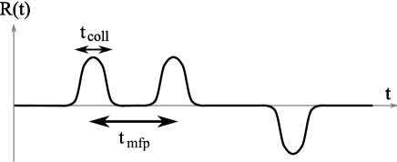
Figure 2: A sample of the stochastic variable $R(t)$, which consists of many pulses randomly distributed.

3.2 A simple model

The collision duration time $t_{\text{coll}}$ can be read off from the random force 2-point function $\kappa(t)={\langle{R(t)R(0)}\rangle}$. To determine the mean-free-path time $t_{\text{mfp}}$, we need higher point functions and some microscopic model which relates those higher point functions with $t_{\text{mfp}}$. Here we propose a simple model  which relates $t_{\text{mfp}}$ with certain 4-point functions of the random force $R$.

For simplicity, we first consider the case with one spatial dimension. Consider a stochastic quantity $R(t)$ whose functional form consists of many pulses randomly distributed. $R(t)$ is assumed to be a classical quantity (c-number). Let the form of a single pulse be $P(t)$. Furthermore, assume that the pulses come with random signs. If we have $k$ pulses at $t=t_{i}$ ($i=1,2,\dots,k$), then $R(t)$ is given by

$$R(t) =\sum_{i=1}^{k}\epsilon_{i}P(t-t_{i}),$$ (3.3)

where $\epsilon_{i}=\pm 1$ are random signs.

Let the distribution of pulses obey the Poisson distribution, which is a physically reasonable assumption if $R$ is caused by random collisions. This means that the probability that there are $k$ pulses in an interval of length $\tau$, say $[0,\tau]$, is given by

$$P_{k}(\tau)=e^{-\mu\tau}{(\mu\tau)^{k}\over k!}.$$ (3.4)

Here, $\mu$ is the number of pulses per unit time. In other words, $1/\mu$ is the average distance between two pulses. We do not assume that the pulses are well separated; namely, we do not assume $\Delta\ll 1/\mu$. If we identify $R(t)$ with the random force in the Langevin equation, $t_{\text{mfp}}=1/\mu$.

The 2-point function for $R$ can be written as

$${\langle{R(t)R(t^{\prime})}\rangle}=\sum_{k=1}^{\infty}e^{-\mu\tau}{(\mu\tau)^{k}\over k!}\sum_{i,j=1}^{k}{\langle{\epsilon_{i}\epsilon_{j}P(t-t_{i})P(t^{\prime}-t_{j})}\rangle}_{k},$$ (3.5)

where we assumed $t,t^{\prime}\in[0,\tau]$ and ${\langle{~{}}\rangle}_{k}$ is the statistical average when there are $k$ pulses in the interval $[0,\tau]$. Because $k$ pulses are randomly and independently distributed in the interval $[0,\tau]$ by assumption, this expectation value is computed as

$$\sum_{i,j=1}^{k}{\langle{\epsilon_{i}\epsilon_{j}P(t-t_{i})P(t^{\prime}-t_{j})}\rangle}_{k}\\ ={1\over\tau^{k}}\int_{0}^{\tau}dt_{1}\cdots dt_{k}\left[\sum_{i=1}^{k}P(t-t_{i})P(t^{\prime}-t_{i})+\sum_{i\neq j}^{k}{\langle{\epsilon_{i}\epsilon_{j}}\rangle}_{k}P(t-t_{i})P(t^{\prime}-t_{j})\right].$$ (3.6)

Here, the second term vanishes because ${\langle{\epsilon_{i}\epsilon_{j}}\rangle}_{k}=0$ for $i\neq j$. Therefore, one readily computes

$$\sum_{i,j=1}{\langle{\epsilon_{i}\epsilon_{j}P(t-t_{i})P(t^{\prime}-t_{j})}\rangle}_{k} ={k\over\tau}\int_{0}^{\tau}dt_{1}P(t-t_{1})P(t^{\prime}-t_{1})$$

$$\approx{k\over\tau}\int_{-\infty}^{\infty}dt_{1}\,P(t-t_{1})P(t^{\prime}-t_{1}).$$ (3.7)

Here, in going to the second line, we took $\tau$ to be much larger than the support of $P(t)$, which is always possible because $\tau$ is arbitrary. Substituting this back into (3.5), we find

$${\langle{R(t)R(t^{\prime})}\rangle}=\mu\int_{-\infty}^{\infty}dt_{1}\,P(t-t_{1})P(t^{\prime}-t_{1}).$$ (3.8)

In a similar way, one can compute the following 4-point function:

$${\langle{R(t)R(t^{\prime})R(t^{\prime\prime})R(t^{\prime\prime\prime})}\rangle}$$

$$=\sum_{k=1}^{\infty}e^{-\mu\tau}{(\mu\tau)^{k}\over k!}\sum_{i,j,m,n=1}^{k}{\langle{\epsilon_{i}\epsilon_{j}\epsilon_{m}\epsilon_{n}P(t-t_{i})P(t^{\prime}-t_{j})P(t^{\prime\prime}-t_{m})P(t^{\prime\prime\prime}-t_{n})}\rangle}_{k}.$$ (3.9)

Again, the expectation value ${\langle{\epsilon_{i}\epsilon_{j}\epsilon_{m}\epsilon_{n}}\rangle}_{k}$ vanishes unless some of $i,j,m,n$ are equal. The possibilities are $i=j\neq m=n$, $i=m\neq j=n$, $i=n\neq j=m$, and $i=j=m=n$. Taking into account all these possibilities, in the end we have

$${\langle{R(t)R(t^{\prime})R(t^{\prime\prime})R(t^{\prime\prime\prime})}\rangle} ={\langle{R(t)R(t^{\prime})R(t^{\prime\prime})R(t^{\prime\prime\prime})}\rangle}_{\text{disc}}+{\langle{R(t)R(t^{\prime})R(t^{\prime\prime})R(t^{\prime\prime\prime})}\rangle}_{\text{conn}},$$ (3.10)

where

$${\langle{R(t)R(t^{\prime})R(t^{\prime\prime})R(t^{\prime\prime\prime})}\rangle}_{\text{disc}} ={\langle{R(t)R(t^{\prime})}\rangle}{\langle{R(t^{\prime\prime})R(t^{\prime\prime\prime})}\rangle}+{\langle{R(t)R(t^{\prime\prime})}\rangle}{\langle{R(t^{\prime})R(t^{\prime\prime\prime})}\rangle}$$

$$\qquad+{\langle{R(t)R(t^{\prime\prime\prime})}\rangle}{\langle{R(t^{\prime})R(t^{\prime\prime})}\rangle},$$ (3.11)

$${\langle{R(t)R(t^{\prime})R(t^{\prime\prime})R(t^{\prime\prime\prime})}\rangle}_{\text{conn}} =\mu\int_{-\infty}^{\infty}du\,P(t-u)P(t^{\prime}-u)P(t^{\prime\prime}-u)P(t^{\prime\prime\prime}-u).$$ (3.12)

We can think of (3.11) as the “disconnected part” and (3.12) as the “connected part”, or non-Gaussianity of the random force statistics.

In the Fourier space, the expressions for these correlation functions simplify:

$${\langle{R(\omega_{1})R(\omega_{2})}\rangle} =2\pi\mu\delta(\omega_{1}+\omega_{2})P(\omega_{1})P(\omega_{2}),$$ (3.13)

$${\langle{R(\omega_{1})R(\omega_{2})R(\omega_{3})R(\omega_{4})}\rangle}_{\text{disc}} =(2\pi\mu)^{2}[\delta(\omega_{1}+\omega_{2})\delta(\omega_{3}+\omega_{4})+\delta(\omega_{1}+\omega_{3})\delta(\omega_{2}+\omega_{4})$$

$$\qquad\qquad+\delta(\omega_{1}+\omega_{4})\delta(\omega_{2}+\omega_{3})]P(\omega_{1})P(\omega_{2})P(\omega_{3})P(\omega_{4}),$$

$${\langle{R(\omega_{1})R(\omega_{2})R(\omega_{3})R(\omega_{4})}\rangle}_{\text{conn}} =2\pi\mu\delta(\omega_{1}+\omega_{2}+\omega_{3}+\omega_{4})P(\omega_{1})P(\omega_{2})P(\omega_{3})P(\omega_{4}).$$ (3.14)

In particular, for small $\omega_{i}$,

$${\langle{R(\omega_{1})R(\omega_{2})}\rangle} \approx 2\pi\mu\delta(\omega_{1}+\omega_{2})P(\omega=0)^{2}$$ (3.15)

$${\langle{R(\omega_{1})R(\omega_{2})R(\omega_{3})R(\omega_{4})}\rangle}_{\text{conn}} \approx 2\pi\mu\delta(\omega_{1}+\omega_{2}+\omega_{3}+\omega_{4})P(\omega=0)^{4}.$$ (3.16)

Therefore, from the small frequency behavior of 2-point function and connected 4-point function, we can separately read off the mean-free-path time $t_{\text{mfp}}\sim 1/\mu$ and $P(\omega=0)$, the impact per collision.

The discussion thus far has been focused on the case with one spatial dimension, but generalization to $n=d-2$ spatial dimensions is straightforward. In this case, the random force becomes an $n$-dimensional vector $R^{I}(t)$, $I=1,2,\dots,n$. Generalizing (3.3), let us model the random force to be given by a sum of pulses:

$$R^{I}(t)=\sum_{i=1}^{k}\epsilon^{I}_{i}P(t-t_{i}).$$ (3.17)

Here, for each value of $i$, $\epsilon^{I}_{i}$ is a stochastic variable taking random values in the $(n-1)$-dimensional sphere $S^{n-1}$. We also assume that $\epsilon^{I}_{i}$ for different values of $i$ are independent of each other. Then we can readily compute the following statistical average:

$${\langle{\epsilon_{i}^{I}\epsilon_{i}^{J}}\rangle}={\delta^{IJ}\over n},\qquad{\langle{\epsilon_{i}^{I}\epsilon_{i}^{J}\epsilon_{i}^{K}\epsilon_{i}^{L}}\rangle}={\delta^{IJ}\delta^{KL}+\delta^{IK}\delta^{JL}+\delta^{IL}\delta^{JK}\over n(n+2)}.$$ (3.18)

From this, we can derive the following $R$-correlators:

$${\langle{R^{I}(\omega_{1})R^{J}(\omega_{2})}\rangle} ={2\pi\mu\over n}\delta^{IJ}\delta(\omega_{1}+\omega_{2})P(\omega_{1})P(\omega_{2}),$$ (3.19)

$${\langle{R^{I}(\omega_{1})R^{J}(\omega_{2})R^{K}(\omega_{3})R^{L}(\omega_{4})}\rangle} ={\langle{R^{I}(\omega_{1})R^{J}(\omega_{2})R^{K}(\omega_{3})R^{L}(\omega_{4})}\rangle}_{\text{conn}}$$

$$\qquad+{\langle{R^{I}(\omega_{1})R^{J}(\omega_{2})R^{K}(\omega_{3})R^{L}(\omega_{4})}\rangle}_{\text{disc}},$$ (3.20)

where

$${\langle{R^{I}(\omega_{1})R^{J}(\omega_{2})R^{K}(\omega_{3})R^{L}(\omega_{4})}\rangle}_{\text{disc}} ={\langle{R^{I}(\omega_{1})R^{J}(\omega_{2})}\rangle}{\langle{R^{K}(\omega_{3})R^{L}(\omega_{4})}\rangle}$$

$$\quad+{\langle{R^{I}(\omega_{1})R^{K}(\omega_{3})}\rangle}{\langle{R^{J}(\omega_{2})R^{L}(\omega_{4})}\rangle}$$

$$\quad+{\langle{R^{I}(\omega_{1})R^{L}(\omega_{4})}\rangle}{\langle{R^{J}(\omega_{2})R^{K}(\omega_{3})}\rangle},$$ (3.21)

$${\langle{R^{I}(\omega_{1})R^{J}(\omega_{2})R^{K}(\omega_{3})R^{L}(\omega_{4})}\rangle}_{\text{conn}} ={2\pi\mu\over n(n+2)}(\delta^{IJ}\delta^{KL}+\delta^{IK}\delta^{JL}+\delta^{IL}\delta^{JK})$$

$$\quad\times\delta(\omega_{1}+\omega_{2}+\omega_{3}+\omega_{4})P(\omega_{1})P(\omega_{2})P(\omega_{3})P(\omega_{4}).$$ (3.22)

These are essentially the same as the $n=1$ results (3.13), (3.14) and we can compute the mean-free-path time $t_{\text{mfp}}\sim 1/\mu$ from the small $\omega$ behavior of 2- and 4-point functions.

One may wonder about the validity of the simple classical model we proposed here, because of the various simplifications and assumptions we made. For example, we assumed that the distribution of pulses is given by the Poisson distribution. This is a natural assumption but, in real systems, different pulses might be correlated and the deviation of the distribution from the Poisson distribution may be appreciable. Also, our model is classical whereas in the real system quantum effects may not be ignorable. In the first place, the kinetic theory picture of independent particles colliding with each other is based on weak coupling intuition and in strongly coupled systems its validity is unclear. However, the simplicity of our model can be regarded as its strength too. Because of its simplicity, our model can be thought of as a zeroth order approximation which correctly captures the essential physics. If a more precise picture of the system is available, we can improve the model and get a better approximation to $t_{\text{mfp}}$, in principle. For strongly coupled plasmas, unfortunately, we do not have such a more precise picture. Still, the relations (3.15), (3.16) must give the qualitatively correct time scale $t_{\text{mfp}}$.

With the above caveats in mind, we will use above relations (3.15), (3.16) to read off $t_{\text{mfp}}$ for the Brownian particle in CFT plasma using the bulk Brownian motion.

3.3 Non-Gaussian random force and Langevin equation

In the above, we argued that the time scale $t_{\text{mfp}}$ that characterizes the statistical properties of the random force $R$ is related to the nontrivial part (connected part) of the 4-point function of $R$. Namely, it is related to the non-Gaussianity of the random force. Here, let us briefly discuss the relation between non-Gaussianity and the non-linear Langevin equation.

In subsection 2.1, we discussed the linear Langevin equation (2.1) for which the friction is proportional to the momentum $p$. In other words, the friction coefficient $\gamma(t)$ did not contain $p$. Furthermore, the random force $R$ was assumed to be Gaussian. In many real systems, Gaussian statistics for the random force gives a good approximation, and the linear Langevin equation provides a useful approach to study the systems. However, this idealized physical situation does not describe nature in general. For example, even the simplest case of a Brownian particle interacting with the molecules of a solvent is rather thought to obey a Poissonian than a Gaussian statistics (just like the simple model discussed in subsection 3.2). It is only in the weak collision limit where energy transfer is relatively small compared to the energy of the system that the central limit theorem says that the statistics can be approximated as Gaussian [46, 47]. Furthermore, due to the non-linear fluctuation-dissipation relations [48], the non-Gaussianity of random force and the non-linearity of friction are closely related. An extension of the phenomenological Langevin equation that incorporates such non-linear and non-Gaussian situations is an issue that has not yet been completely settled (for a recent discussion, see [47]).

However, the relation between time scales $t_{\text{coll}}$, $t_{\text{mfp}}$ and $R$ correlators derived in subsection 3.2 does not depend on the existence of such an extension of the Langevin equation. Below, we will compute $R$ correlators using the AdS/CFT correspondence and derive expressions for the time scale $t_{\text{mfp}}$, but that derivation will not depend on the existence of an extended Langevin equation either. It would be interesting to use the concrete AdS/CFT setup for Brownian motion to investigate the above issue of a non-linear non-Gaussian Langevin equation. We leave it for future research.

4 Holographic computation of the $R$-correlator

In the last section, we saw that $t_{\text{mfp}}$ can be read off if we know the low-frequency limit of the 2- and 4-point functions of the random force. For the connected 4-point function to be nonvanishing, we need more than the quadratic term $S_{0}$ in (2.12) or (2.41). Such terms will arise if we keep higher order terms in the expansion of the Nambu–Goto action. This amounts to taking into account the relativistic correction to the motion of the “cloud” around the quark mentioned in subsection 2.2. In the case of the neutral black holes discussed in subsection 2.2, if we keep up to quartic terms (and drop a constant), the action becomes

$$S =S_{0}+S_{\text{int}},$$ (4.1)

$$S_{\text{int}} ={1\over 16\pi{\alpha^{\prime}}}\int dt\,dr\biggl{(}{\dot{X}^{2}\over f}-{r^{4}f}X^{\prime 2}\biggr{)}^{2},$$ (4.2)

where the quadratic (free) part $S_{0}$ is as given before in (2.12).

There are two ways to compute correlation functions in the presence of the quartic term (4.2). The first one, which is perhaps more intuitive, is to regard the theory with the action $S_{0}+S_{\text{int}}$ as a field theory of the worldsheet field $X$ at temperature $T$ and compute the $X$ correlators using the standard technique of thermal field theory [49]. The second one, which is perhaps more rigorous but technically more involved, is to use the GKPW prescription [5, 6] and holographic renormalization [27] to compute the correlator for the force acting on the boundary Brownian particle.

The two approaches give essentially the same result in the end, as they should. In the following, we will first describe the first approach and then briefly discuss the the second approach, relegating the technical details to Appendix D. In this section and the next, for the simplicity of presentation, we will focus on the neutral black holes of subsection 2.2.

4.1 Thermal field theory on the worldsheet

The Brownian string we are considering is immersed in a black hole background which has temperature $T$ given by (2.11). Therefore, we can think of the string described by the action (4.1) just as a field theory of $X(t,r)$ at temperature $T$, for which the standard thermal perturbation theory (see e.g. [49]) is applicable.

For the thermal field theory described by (4.1), let us compute the real-time connected 4-point function

$$G^{(x)}_{\text{conn}}(t_{1},t_{2},t_{3},t_{4}) ={\langle{{\cal T}[x(t_{1})x(t_{2})x(t_{3})x(t_{4})]}\rangle}_{\text{conn}}$$

$$={\langle{{\cal T}[X(t_{1},r_{c})X(t_{2},r_{c})X(t_{3},r_{c})X(t_{4},r_{c})]}\rangle}_{\text{conn}},$$ (4.3)

where ${\cal T}$ is the time ordering operator and $x(t)=X(t,r_{c})$ is the position of the boundary Brownian particle. In the absence of external force, $K(\omega)=0$, (2.6) relates $x$ and random force $R$ by

$$R(\omega)=-{im\omega x(\omega)\over\mu(\omega)}.$$ (4.4)

Therefore, using the low-frequency expression for $\mu(\omega)$ given in (2.33), we can compute the 4-point function of $R$ from the one for $x$ in (4.3).

Figure 3: The contour for computing real-time correlators at finite temperature.

As is standard, we can compute such real-time correlators at finite temperature $T$ by analytically continuing the time $t$ to a complex time $z$ and performing path integration on the complex $z$ plane along the contour $C=C_{1}+C_{2}+C_{3}$, where $C_{i}$ are oriented intervals

$$C_{1}=[-L,L],\qquad C_{2}=[L,-L],\qquad C_{3}=[-L,-L-i\beta]$$ (4.5)

as shown in Figure 3. $L$ is a large positive number which is sent to infinity at the end of computation. We can parametrize the contour $C$ by a real parameter $\lambda$ which increases along $C$ as

$$\begin{array}[]{rll}C_{1}:&\qquad z=\lambda-L&\qquad(0\leq\lambda\leq 2L)\\ C_{2}:&\qquad z=3L-\lambda&\qquad(2L\leq\lambda\leq 4L)\\ C_{3}:&\qquad z=-L+i(4L-\lambda)&\qquad(4L\leq\lambda\leq 4L+\beta)\end{array}$$ (4.9)

The field $X$ is defined for all values of $\lambda$. Another convenient parametrization of $C$ is

$$\begin{array}[]{rll}C_{1}:&\qquad z=t,&\qquad(-L\leq t\leq L),\\ C_{2}:&\qquad z=t,&\qquad(-L\leq t\leq L),\\ C_{3}:&\qquad z=-L-i\tau,&\qquad(0\leq\tau\leq\beta).\end{array}$$ (4.13)

We will denote by $X_{[i]}$ ($i=1,2,3$) the field $X$ on the segment $C_{i}$ parametrized by $t$ and $\tau$ in (4.13). Henceforth, we will use the subscript $[i]$ for a quantity associated with $C_{i}$.

The path integral is now performed over $X_{[1]}(t)$, $X_{[2]}(t)$, and $X_{[3]}(\tau)$, but in the $L\to\infty$ limit the path integral over $X_{[3]}$ factorizes and can be dropped [49]. Therefore, with the parametrization (4.13), the path integral becomes

$$\int{\cal D}X\,e^{iS}\to\int{\cal D}X_{[1]}\,{\cal D}X_{[2]}\,e^{i(S_{[1]}-S_{[2]})},$$ (4.14)

where $S_{[i]}$, $i=1,2$ are obtained by replacing $X$ with $X_{[i]}$ in (4.1). The negative sign in front of $S_{[2]}$ in (4.14) is because the direction of the parameter $t$ we took in (4.13) is opposite to that of $C_{2}$.

The correlator (4.3) can be written as

$$G^{(x)}_{\text{conn}}(t_{1},t_{2},t_{3},t_{4})={\langle{{\cal T}_{C}[X_{[1]}(t_{1},r_{c})X_{[1]}(t_{2},r_{c})X_{[1]}(t_{3},r_{c})X_{[1]}(t_{4},r_{c})]}\rangle}_{\text{conn}},$$ (4.15)

where ${\cal T}_{C}$ is ordering along $C$ (in other words, with respect to the parameter $\lambda$), and can be computed in perturbation theory by treating $S_{0}$ as the free part and $S_{\text{int}}$ as an interaction. In doing that, we have to take into account both the type-1 fields $X_{[1]}$ and the type-2 fields $X_{[2]}$. Namely, we have to introduce propagators not just for $X_{[1]}$ but also between $X_{[1]}$ and $X_{[2]}$ as follows

$$\begin{split}D_{[11]}(t-t^{\prime},r,r^{\prime})&={\langle{{\cal T}_{C}[X_{[1]}(t,r)X_{[1]}(t^{\prime},r^{\prime})]}\rangle}_{0}={\langle{{\cal T}[X(t,r)X(t^{\prime},r^{\prime})]}\rangle}_{0}=D_{F}(t-t^{\prime},r,r^{\prime}),\\ D_{[21]}(t-t^{\prime},r,r^{\prime})&={\langle{{\cal T}_{C}[X_{[2]}(t,r)X_{[1]}(t^{\prime},r^{\prime})]}\rangle}_{0}={\langle{X(t,r)X(t^{\prime},r^{\prime})]}\rangle}_{0}=D_{W}(t-t^{\prime},r,r^{\prime}).\end{split}$$ (4.16)

Here, ${\langle{\,}\rangle}_{0}$ is the expectation value for the free theory with action $S_{0}$ at temperature $T$. We see that the propagators $D_{[11]}$ and $D_{[21]}$ are equal, respectively, to the usual time-ordered (Feynman) propagator $D_{F}$ and the Wightman propagator $D_{W}$ of the field $X(t,r)$. We must also remember that we have not only interaction vertices that come from $S^{\text{int}}_{[1]}$ and involve $X_{[1]}$, but also ones that come from $S^{\text{int}}_{[2]}$ and involve $X_{[2]}$. The second type of vertices come with an extra minus sign.

Using the propagators (4.16), the connected 4-point function is evaluated, at leading order in perturbation theory, to be

$$G^{(x)}_{\text{conn}}(\omega_{1},\omega_{2},\omega_{3},\omega_{4})={i\over 16\pi{\alpha^{\prime}}}2\pi\delta(\omega_{1}+\cdots+\omega_{4})\int_{r_{H}}^{r_{c}}dr\,$$

$$\times\Biggl{\{}\sum_{\text{perm}\atop(ijkl)}\Biggl{[}{\omega_{i}\omega_{j}\over f}D_{[11]}(\omega_{i})D_{[11]}(\omega_{j})+{r^{4}f}\partial_{r}D_{[11]}(\omega_{i})\partial_{r}D_{[11]}(\omega_{j})\Biggr{]}$$

$$\qquad\qquad\times\Biggl{[}{\omega_{k}\omega_{l}\over f}D_{[11]}(\omega_{k})D_{[11]}(\omega_{l})+{r^{4}f}\partial_{r}D_{[11]}(\omega_{k})\partial_{r}D_{[11]}(\omega_{l})\Biggr{]}-(D_{[11]}\to D_{[21]})\Biggr{\}}.$$ (4.17)

Here, we wrote down the result in the Fourier space and used a shorthand notation $D_{[11]}(\omega_{i})\equiv D_{[11]}(\omega_{i},r,r_{c})$. The summation is over permutations $(ijkl)$ of $(1234)$.

We are interested in the low frequency limit of this correlator. In that limit, the propagators simplify and can be explicitly written down. In Appendix C, we study the low-frequency propagators, and the resulting expressions are

$$\begin{split}D_{[11]}(\omega,r,r_{c})&=D_{F}(\omega,r,r_{c})={2\pi{\alpha^{\prime}}\over r_{H}^{2}}\left[{e^{i\omega r_{*}}+e^{-i\omega r_{*}}\over\omega(1-e^{-\beta\omega})}-{e^{i\omega r_{*}}\over\omega}\right],\\[4.30554pt] D_{[21]}(\omega,r,r_{c})&=D_{W}(\omega,r,r_{c})={2\pi{\alpha^{\prime}}\over r_{H}^{2}}{e^{i\omega r_{*}}+e^{-i\omega r_{*}}\over\omega(1-e^{-\beta\omega})},\end{split}$$ (4.18)

where $r_{*}$ is the tortoise coordinate introduced in (2.19). As explained in (B.21), the precise low frequency limit we are taking is

$$\omega_{i}\to 0,\qquad\qquad\beta,~{}\omega_{i}r_{*}:~{}\text{fixed}.$$ (4.19)

The reason why we have to keep $\omega_{i}r_{*}$ fixed is that, no matter how small $\omega_{i}$ is, we can consider a region very close to the horizon ($r_{*}=-\infty$) such that $\omega_{i}r_{*}={\cal O}(1)$. If we insert the expressions (4.18) into (4.17) and keep the leading term in the small $\omega_{i}$ expansion in the sense of (4.19), we obtain

$$G^{(x)}_{\text{conn}}(\omega_{1},\omega_{2},\omega_{3},\omega_{4}) \sim{i{\alpha^{\prime}}^{3}\beta^{5}\over\omega_{1}\omega_{2}\omega_{3}\omega_{4}}\delta(\omega_{1}+\cdots+\omega_{4})$$

$$\qquad\times\sum_{1\leq i<j\leq 4}(\omega_{i}+\omega_{j})\int_{-\infty}^{0}dr_{*}\,{r^{2}\over f}e^{-2i(\omega_{i}+\omega_{j})r_{*}}+{\cal O}(\omega^{-2}),$$ (4.20)

where we ignored numerical factors. Using (4.4) and (2.33), we can finally derive the expression for the $R$ correlator:

$$G^{(R)}_{\text{conn}}(\omega_{1},\omega_{2},\omega_{3},\omega_{4}) \sim{i\over{\alpha^{\prime}}\beta^{3}}\delta(\omega_{1}+\cdots+\omega_{4})$$

$$\qquad\times\sum_{1\leq i<j\leq 4}(\omega_{i}+\omega_{j})\int_{-\infty}^{0}dr_{*}\,{r^{2}\over f}e^{-2i(\omega_{i}+\omega_{j})r_{*}}+{\cal O}(\omega^{2}).$$ (4.21)

Let us look at the IR part of (4.20), namely the contribution from the near-horizon region (large negative $r_{*}$). Because $f\sim(d-1)e^{(d-1)r_{H}r_{*}}$ near the horizon, the $r_{*}$ integral in (4.20) is

$$\int_{-\infty}^{0}dr_{*}\,{r^{2}\over f}e^{-2i(\omega_{i}+\omega_{j})r_{*}}\sim{r_{H}^{2}\over d-1}\int_{-\infty}dr_{*}\,e^{-(d-1)r_{H}r_{*}}e^{-2i(\omega_{i}+\omega_{j})r_{*}}$$ (4.22)

which diverges because of the contribution from the near horizon region, $r_{*}\to-\infty$. We will discuss the nature of this IR divergence later.

4.2 Holographic renormalization

Next, let us discuss another way to compute the correlators of the boundary Brownian motion, following the standard GKPW procedure [5, 6]. For this approach, we send the UV cutoff $r_{c}\to\infty$ and let the string extend all the way to the AdS boundary $r=\infty$. The boundary value of $X(t,r)$ is the position of the boundary Brownian particle: $x(t)=X(t,r\to\infty)$. The boundary operator dual to the bulk field $X(t,r)$ is $F(t)$, the total force (friction plus random force) acting on the boundary Brownian particle. The AdS/CFT dictionary

$${\left\langle{e^{i\int dt\,F(t)x(t)}}\right\rangle}_{\text{CFT}}=e^{iS_{\text{bulk}}[x(t)]}$$ (4.23)

says that, to compute boundary correlators for $F$, we should consider bulk configurations for which $X(t,r)$ asymptotes to a given function $x(t)$ at $r=\infty$, evaluate the bulk action, and functionally differentiate the result with respect to $x(t)$. Note that, in the limit $r_{c}\to\infty$ or $m\to\infty$ that we take, friction is ignorable as compared to random force $R$, and $F$ correlators are the same as $R$ correlators [12]. Roughly speaking, because the Brownian particle does not move in the $m\to\infty$ limit, there will be no friction and thus $R=F$.

In the end, the resulting 4-point function ${\langle{FFFF}\rangle}$ is essentially given by the interaction term in the action, with the $X$ fields replaced by the boundary-bulk propagators. Namely,

$${\langle{{\cal T}[F(t_{1})F(t_{2})F(t_{3})F(t_{4})]}\rangle} \sim{1\over 16\pi{\alpha^{\prime}}}\int dt\,dr\sum_{\text{perm}\atop(ijkl)}\left[-{\partial_{t}K(t_{i})\,\partial_{t}K(t_{j})\over f}+{r^{4}f}\,\partial_{r}K(t_{i})\,\partial_{r}K(t_{j})\right]$$

$$\qquad\times\left[-{\partial_{t}K(t_{k})\,\partial_{t}K(t_{l})\over f}+{r^{4}f}\,\partial_{r}K(t_{k})\,\partial_{r}K(t_{l})\right],$$ (4.24)

where $K(t_{i})\equiv K(t,r|t_{i})$ is the boundary-bulk propagator from the boundary point $t_{i}$ to the bulk point $(t,r)$. This is the Witten diagram rule that we naively expect. However, because the worldvolume theory of a string is different from, e.g. a Klein–Gordon scalar, a careful consideration of holographic renormalization (see [27] for a review) is necessary. Indeed, the naive expression is (4.24) is UV divergent and needs regularization. Furthermore, our black hole spacetime is a Lorentzian geometry and we should apply the rules of Lorentzian AdS/CFT [28, 29]. As is explained in Appendix D, after all the dust has been settled, the $F$ correlator gives exactly the same IR divergence as the naive computation of the $R$ correlator, (4.21). This implies that this IR divergence we are finding is not an artifact but a real thing to be interpreted physically.

It is worth pointing out that the result (4.24) has a similar structure to the one we saw in the toy model (3.12), with the propagator $K(t)$ roughly corresponding to $P(t)$. It would be interesting to find an improved toy model which precisely reproduces the structure (4.24).

In Appendix D.5, we also computed the retarded 4-point function of random force. The expression is free from both IR and UV divergences and the final result is finite. However, because we do not know how to relate the retarded 4-point function and $t_{\text{mfp}}$, this cannot be used to compute $t_{\text{mfp}}$. It would be interesting to find a microscopic model that directly relates retarded correlators and $t_{\text{mfp}}$.

4.3 General polarizations

The argument so far has been as if there were only one field $X$ and the associated random force $R$. However, in the general $d>3$ case we have $n=d-2>1$ fields $X^{I}$, $I=1,2,\dots,n$. Considering all $X^{I}$, the bulk action (4.2) actually becomes

$$S_{\text{int}} ={1\over 16\pi{\alpha^{\prime}}}\int dt\,dr\biggl{[}{(\dot{X}^{I})^{2}\over f}-{r^{4}f}\,(X^{I}{}^{\prime})^{2}\biggr{]}^{2}.$$ (4.25)

The associated random force $R^{I}$ has $n$ components too.

The computation of 4-point functions in this multi-component case can be done completely in parallel with the one-component case. Let us define

$$G^{(x)IJKL}_{\text{conn}}(t_{1},t_{2},t_{3},t_{4})\equiv{\langle{{\cal T}[X^{I}(t_{1},r_{c})X^{J}(t_{2},r_{c})X^{K}(t_{3},r_{c})X^{L}(t_{4},r_{c})]}\rangle}.$$ (4.26)

This is nonvanishing only if some indices are identical. More precisely, the only nonvanishing cases are (i) all indices are identical, $I=J=K=L$, or (ii) indices are pairwise identical, $I=J\neq K=L$, $I=K\neq J=L$, or $I=L\neq J=K$.

In case (i), the resulting 4-point function is exactly the same as the one-component case (4.17). Consequently, the IR form of the random force correlator $G^{(R)IIII}_{\text{conn}}$ is the same as the one-component case (4.21).

In case (ii), on the other hand, the 4-point function becomes

$$G^{(x)IIJJ}_{\text{conn}}(\omega_{1},\omega_{2},\omega_{3},\omega_{4})={i\over 16\pi{\alpha^{\prime}}}2\pi\delta(\omega_{1}+\cdots+\omega_{4})\int_{r_{H}}^{r_{c}}dr\,$$

$$\times\Biggl{\{}8\Biggl{[}{\omega_{1}\omega_{2}\over f}D_{[11]}(\omega_{1})D_{[11]}(\omega_{2})+{r^{4}f}\partial_{r}D_{[11]}(\omega_{1})\partial_{r}D_{[11]}(\omega_{2})\Biggr{]}$$

$$\qquad\qquad\times\Biggl{[}{\omega_{3}\omega_{4}\over f}D_{[11]}(\omega_{3})D_{[11]}(\omega_{4})+{r^{4}f}\partial_{r}D_{[11]}(\omega_{3})\partial_{r}D_{[11]}(\omega_{4})\Biggr{]}-(D_{[11]}\to D_{[21]})\Biggr{\}}.$$ (4.27)

The IR form of the random force correlator is

$$G^{(R)IIJJ}_{\text{conn}}(\omega_{1},\omega_{2},\omega_{3},\omega_{4}) \sim{i\over{\alpha^{\prime}}\beta^{3}}\delta(\omega_{1}+\cdots+\omega_{4})\,\int_{-\infty}^{0}dr_{*}\,{r^{2}\over f}$$

$$\qquad\times\sum_{1\leq i\leq 2,\,3\leq j\leq 4}(\omega_{i}+\omega_{j})e^{-2i(\omega_{i}+\omega_{j})r_{*}}+{\cal O}(\omega^{2}).$$ (4.28)

Comparing this with the expectation from the field theory side, (3.22) we observe the same structure. Namely, the connected 4-point functions are nonvanishing only when the polarization indices are all or pairwise identical. The precise relative values of the nonvanishing 4-point functions are model-dependent and not important; in the simple model of subsection 3.2, it depends on our choice of the expectation values (3.18).

4.4 Comment on the basis

In this section, we computed the correlation functions for type-1 fields $X_{[1]}$, such as (4.15), as the quantities to be matched with those in the simple model presented in subsection 3.2. One may wonder whether it is more appropriate to use correlation functions in some other basis, such as the retarded/advanced ($r$-$a$) basis [50, 51, 52]. For example, $G_{rrrr}$ in the $r$-$a$ basis has no knowledge of time ordering unlike $G_{[1111]}$ in the 1-2 basis and might seem more natural quantity to consider. However, recall that the analysis in subsection 3.2 is a classical one; therefore, the difference between $G_{[1111]}$ and $G_{rrrr}$ is quantum and thus negligible in our approximation. Clearly, $G_{[1111]}$ is much easier to compute than $G_{rrrr}$ and we will use the former to extract $t_{\rm mfp}$ below.

5 The IR divergence

In the last section, we computed the connected 4-point function for the random force $R$ and found that the low-frequency expression,

$$G^{(R)}_{\text{conn}}(\omega_{1},\omega_{2},\omega_{3},\omega_{4}) \sim{i\over{\alpha^{\prime}}\beta^{3}}\delta(\omega_{1}+\cdots+\omega_{4})$$

$$\qquad\times\sum_{1\leq i<j\leq 4}(\omega_{i}+\omega_{j})\int_{-\infty}^{0}dr_{*}\,{r^{2}\over f}e^{-2i(\omega_{i}+\omega_{j})r_{*}},$$ (5.1)

has an IR divergence coming from the integral in the near horizon region. What is the physical reason for this divergence? Very near the horizon, the expansion of the Nambu–Goto action in the transverse fluctuation $X$ breaks down because the proper temperature becomes higher and higher as one approaches the horizon and, as a result, the string fluctuation gets wilder and wilder. The correct thing to do in principle is to consider the full non-linear Nambu–Goto action, but this is technically very difficult. Instead, a physically reasonable estimate of the result is the following. Let us introduce an IR cutoff near the horizon at

$$r_{\rm s}=r_{H}+\epsilon,$$ (5.2)

where $\epsilon\ll r_{H}$. We take this cutoff $r_{\rm s}$ to be the radius where the expansion of the Nambu–Goto action becomes bad. Then, in IR-divergent expressions such as (4.21), we simply throw away the contribution from the region $r<r<r_{\rm s}$ by taking the integral to be only over $r>r_{\rm s}$. Of course, to obtain a more precise result, we should include the contribution from the region $r_{H}<r<r_{\rm s}$ with the higher order terms in the expansion of the Nambu–Goto action taken into account. However, we expect that the contribution from this region $r_{H}<r<r_{\rm s}$ will be of the same order as the contribution from the region $r>r_{\rm s}$ and, therefore, we can estimate the full result by just keeping the latter contribution.

With this physical expectation in mind, let us evaluate the mean-free-path time $t_{\text{mfp}}$ by introducing the IR cutoff (5.2). The parameter $\epsilon$ appearing in (5.2) can be related to the proper distance from the horizon, $s$, as follows:

$$s=\int_{r_{H}}^{r_{H}+\epsilon}{dr\over r\sqrt{f}}\sim\int_{r_{H}}^{r_{H}+\epsilon}{dr\over\sqrt{(d-1)r_{H}(r-r_{H})}}=\sqrt{2\epsilon\over(d-1)r_{H}}.$$ (5.3)

Therefore

$$\epsilon\sim s^{2}r_{H},$$ (5.4)

where we dropped numerical factors. In the tortoise coordinate $r_{*}$, the cutoff is at

$$r_{*}^{\rm s}\sim-{1\over(d-1)r_{H}}\log s^{2},$$ (5.5)

where we used (2.20).

The introduction of an IR cutoff of the geometry near the horizon also means that the resulting expressions such as (5.1), with the IR cutoff imposed, is valid only for frequencies larger than a certain cutoff frequency $\omega_{\rm s}$. We can relate $\omega_{\rm s}$ with the geometric cutoff $r_{*}^{\rm s}$ as follows. If we cut off the geometry at $r_{*}=r_{*}^{\rm s}$, we have to impose some boundary condition there (just as for the brick wall model). For example, let us impose a Neumann boundary condition. As was shown in (B.19), for very low frequencies, the solutions to the wave equation behave as

$$f_{\omega}(r)\sim e^{i\omega r_{*}}+e^{-i\omega r_{*}}.$$ (5.6)

For this to satisfy Neumann boundary condition $\partial_{r_{*}}f_{\omega}(r)|_{r_{*}=r_{*}^{\rm s}}=0$, we need $\omega={n\pi/r_{*}^{\rm s}}$ where $n\in{\mathbb{Z}}$. Namely, the frequency has been discretized in units of $\pi/|r_{*}^{\rm s}|$. Therefore, the smallest possible frequency is

$$\omega_{\rm s}\sim{1\over|r_{*}^{s}|}\sim{1\over\beta\log(1/s)}.$$ (5.7)

If we use (5.5) and (5.7), the correlator (5.1) becomes

$$G^{(R)}_{\text{conn}}(\omega_{1},\omega_{2},\omega_{3},\omega_{4}) \sim{i\over{\alpha^{\prime}}\beta^{3}}\delta(\omega_{1}+\cdots+\omega_{4})\,\omega_{\rm s}r_{H}^{2}\int_{r_{*}^{\rm s}}dr_{*}e^{-(d-1)r_{H}r_{*}}$$

$$\sim{i\over{\alpha^{\prime}}\beta^{3}}\delta(\omega_{1}+\cdots+\omega_{4})\,\omega_{\rm s}r_{H}^{2}\,{e^{-(d-1)r_{H}r_{*}^{\rm s}}\over r_{H}}$$

$$\sim{is^{2}\omega_{\rm s}\over{\alpha^{\prime}}\beta^{4}}\delta(\omega_{1}+\cdots+\omega_{4})\sim{is^{2}\over{\alpha^{\prime}}\beta^{5}\log(1/s)}\delta(\omega_{1}+\cdots+\omega_{4}).$$ (5.8)

On the other hand, from (2.35), the 2-point function is

$$G^{(R)}(\omega_{1},\omega_{2}) \sim{1\over{\alpha^{\prime}}\beta^{3}}\delta(\omega_{1}+\omega_{2})$$ (5.9)

Comparing above results and the toy model results (3.15), (3.16), we obtain

$$t_{\rm mfp}\sim{1\over\mu}\sim{{\alpha^{\prime}}\beta\over s^{2}\log(1/s)},\qquad P(\omega=0)\sim{1\over\beta s\sqrt{\log(1/s)}}.$$ (5.10)

Now the question is how to determine the length $s$. This must be the place where the expansion (4.1) of the Nambu–Goto action becomes bad. One can show that this occurs a proper length $\sim\sqrt{{\alpha^{\prime}}}$ away from the horizon due to thermal fluctuation (Hawking radiation) in the black hole background (for an argument in more general setups see subsection 6.1). This leads us to set

$$s\sim\sqrt{{\alpha^{\prime}}}.$$ (5.11)

At this point, the local proper temperature becomes of the order of the Hagedorn temperature, $\sim 1/\sqrt{{\alpha^{\prime}}}$. The above condition must be the same as the condition that the loop correction of the worldsheet theory to the 4-point function ${\langle{F^{4}}\rangle}$ becomes of the same order as the tree level contribution.

If we substitute (5.11) into (5.10), we obtain

$$t_{\rm mfp}\sim{1\over T\log\lambda},\qquad P(\omega=0)\sim{T\lambda^{1/4}\over\sqrt{\,\log\lambda}}$$ (5.12)

where, following the convention of the $d=5$ (AdS₅) case, we defined the “’t Hooft coupling” by

$$\lambda\equiv{l^{4}\over{\alpha^{\prime}}^{2}},$$ (5.13)

where we restored the AdS radius $l$ which we have been setting to one.

The result (5.12) is quite interesting. In [21], the collision duration time $t_{\text{coll}}$ was determined to be

$$t_{\text{coll}}\sim{1\over T}.$$ (5.14)

Therefore, $t_{\text{mfp}}$ given in (5.12) implies that a plasma particle can be thought of as in interaction with roughly $\log\lambda$ other particles simultaneously.

Even if we take into account the fact that $X^{I}$ has in general more than one component $(I=1,2,\dots,n=d-2)$ and use the results such as (3.22), (4.28), we end up the same estimate for $t_{\text{mfp}}$ as far as its order is concerned.

6 Generalizations

In the previous section, we derived using AdS/CFT the expression for the mean-free-path time $t_{\text{mfp}}$ for the simple case of neutral plasma. In this section, we sketch how this generalizes to the more general metric (2.36) and present the expression for the mean-free-path time for more general systems such as charged plasmas. As an example, we will apply the result to the STU black hole.

6.1 Mean-free-path time for the general case

We are interested in computing the mean-free-path time in field theory by analyzing the motion of a Brownian string in the metric (2.36). For that, as has been explained in section 3 for the neutral case, we need to compute the 4-point function of the random force in addition to the 2-point function.

Expanding the Nambu–Goto action in the background metric (2.36) up to quartic order, the action for the string in the tortoise coordinate defined in (2.43) is given as follows:

$$S =S_{0}+S_{\text{int}},$$ (6.1)

$$S_{0} =\frac{1}{4\pi\alpha^{\prime}}\int dt\,dr_{*}\,G\,(\dot{X}^{2}-X^{\prime 2}),$$ (6.2)

$$S_{\text{int}} =\frac{1}{16\pi\alpha^{\prime}}\int dt\,dr_{*}\,{G^{2}\over h_{t}f}(\dot{X}^{2}-X^{\prime 2})^{2},$$ (6.3)

where we dropped a constant independent of the field $X$, and $\,\dot{}=\partial_{t}$, ${}^{\prime}=\partial_{r_{*}}$. As we discussed in subsection 4.2 for the simple neutral case, we can use $S_{\text{int}}$ as the interaction term and apply the usual GKPW rule to compute correlators for the random force  $F$ dual to the bulk field $X$. As before, the naive result from the GKPW prescription includes both UV and IR divergences. Using holographic renormalization, which is discussed in Appendix D for the neutral case, we can remove the UV divergence by adding counter terms to the action. The IR divergence, on the other hand, signals the breakdown of the quartic approximation (6.1). We regulate this divergence by introducing an IR cutoff at $r_{*}=r_{*}^{s}$ near to the horizon, whose physical motivation was explained in section 5.

Following the same analysis as in section 5 now with the interaction term (6.3), we obtain an expression similar to (4.21) for the connected random force 4-point function. The dominant contribution comes from the near-horizon region and is given in frequency space by

$${\langle{{\cal T}[F^{4}]}\rangle}_{\text{conn}} \sim{i\over\alpha^{\prime}\beta^{3}}\delta(\omega_{1}+\cdots+\omega_{4})\int_{r^{s}_{*}}dr_{*}{G^{2}\over fh_{t}}\sum\limits_{1\leq i<j\leq 4}(\omega_{i}+\omega_{j})e^{-2i(\omega_{i}+\omega_{j})r_{*}},$$ (6.4)

where $r_{*}^{\rm s}$ is the aforementioned IR cutoff (in the tortoise coordinate). Let the IR cutoff in the $r$ coordinate be at $r=r_{H}+\epsilon\equiv r_{\rm s}$. The parameter $\epsilon$ is related to the proper distance $s$ from the horizon as

$$s=\int^{r_{H}+\epsilon}_{r_{H}}\sqrt{h_{r}\over f\,}\,dr\approx\sqrt{{2\epsilon\,h_{r}(r_{H})\over k_{H}}},\qquad\epsilon\approx{s^{2}k_{H}\over 2h_{r}(r_{H})}.$$ (6.5)

Using the relation (2.43) between $r_{\rm s}$ and $r_{*}^{\rm s}$, we can estimate the cut-off integral (6.4) as

$${\langle{\mathcal{T}[F^{4}]}\rangle} \sim{G^{2}(r_{H})\,\omega_{\rm s}\over\alpha^{\prime}s^{2}}\delta(\omega_{1}+\cdots+\omega_{4}),$$ (6.6)

where $\omega_{\rm s}$ is the smallest frequency for which the expansion (6.1) is valid. Combining this with the result (2.49) for the 2-point function, the mean-free-path time is estimated as

$$t_{\rm mfp}\sim{\alpha^{\prime}\beta^{2}\omega_{\rm s}\over s^{2}}.$$ (6.7)

Now, let us determine the IR cutoff parameters $s$ (or equivalently $\epsilon$) and $\omega_{\rm s}$ appearing in (6.7). As before, we take the IR cutoff to be the location where $S_{0}$ and $S_{\text{int}}$ become of the same order. As is clear from (6.2), (6.3), the expansion of the Nambu–Goto action becomes bad at the location where

$${G\over h_{t}f}\dot{X}^{2},~{}{G\over h_{t}f}X^{\prime 2}\sim 1.$$ (6.8)

So, we would like to estimate $\dot{X}$, $X^{\prime}$. Near the horizon, $r\approx r_{H}$, we can write the action (6.2) as

$$S_{0}\sim\frac{1}{2}\int dt\,dr_{*}(\dot{{\widetilde{X}}}^{2}-{\widetilde{X}}^{\prime 2}),\qquad{\widetilde{X}}\equiv\sqrt{G(r_{H})\over 2\pi\alpha^{\prime}}\,X.$$ (6.9)

There being no dimensional quantity in the problem other than the temperature $T$, we must have $\dot{{\widetilde{X}}},{\widetilde{X}}^{\prime}\sim T$, namely $|\dot{X}|,|X^{\prime}|\sim\sqrt{2\pi\alpha^{\prime}/G(r_{H})\,}\,T$. So, the condition (6.8) determines the IR cutoff to be at

$$r-r_{H}=\epsilon\sim{\alpha^{\prime}T^{2}\over k_{H}h_{t}(r_{H})}.$$ (6.10)

In term of $s$, the IR cutoff is at the string length:

$$s\sim\sqrt{\alpha^{\prime}}.$$ (6.11)

It is more subtle to determine the parameter $\omega_{\rm s}$. In Appendix B (around Eq. (B.16)), the following was shown. Let us we choose the tortoise coordinate $r_{*}$ to be related to $r$ near the horizon as

$$r_{*}\approx{1\over 4\pi T}\log\left({r-r_{H}\over L_{H}}\right),$$ (6.12)

where $L_{H}$ is defined through the following integral

$$\int_{\infty}^{r}{dr\over fG}\sqrt{h_{r}\over h_{t}}={1\over 4\pi G_{H}T}\log\left({r-r_{H}\over L_{H}}\right)+{\cal O}(r-r_{H})$$ (6.13)

for $r\approx r_{H}$. Then the solution $f_{\omega}(r)$ to the wave equation (2.42), satisfying a normalizable boundary condition at infinity, will have the form

$$f_{\omega}(r)\sim e^{i\omega r_{*}}-e^{-i\omega r_{*}}$$ (6.14)

for small $\omega$. More precisely, we have

$$f_{\omega}(r)\sim e^{i\omega r_{*}}-e^{i\alpha_{\omega}}e^{-i\omega r_{*}},\qquad\alpha_{\omega}={\cal O}(\omega^{2}).$$ (6.15)

Now, let us we impose some boundary condition at $r_{*}^{\rm s}$, such as a Neumann boundary condition $\partial_{r_{*}}f_{\omega}=0$, then the frequency $\omega$ gets discretized in units of $\Delta\omega=\pi/|r_{*}^{\rm s}|$. Note that, if $\alpha_{\omega}={\cal O}(\omega)$ as $\omega\to 0$, then the coefficient of the ${\cal O}(\omega)$ term will affect the value of $\Delta\omega$; this is why (6.15) was important. This motivates the following choice for the minimum frequency:

$$\omega_{\rm s}\sim\Delta\omega\sim{1\over|r_{*}^{\rm s}|}\sim{1\over\beta\log\left({L_{H}\over\epsilon}\right)}\sim{1\over\beta\log\left({\beta L_{H}\over s^{2}}\sqrt{h_{t}(r_{H})h_{r}(r_{H})}\right)}.$$ (6.16)

Substituting in the above expressions for $s,\omega_{\rm s}$, the mean-free-path time (6.7) is

$$t_{\text{mfp}}\sim{1\over T\log\bigl{(}\eta\sqrt{\lambda}\bigr{)}},\qquad\qquad\eta\equiv{L_{H}\over T}\sqrt{h_{t}(r_{H})h_{r}(r_{H})\,},$$ (6.17)

where $\lambda$ is the “’t Hooft coupling” defined in (5.13). Note that the nontrivial effect of charge only enters through the logarithm and hence the dependence of $t_{\text{mfp}}$ on it is very mild in the strongly coupled case $\lambda\gg 1$.

6.2 Application: STU black hole

The AdS/CFT correspondence has been successfully used to extract the properties of field theory plasmas. A particularly interesting case is a 4-dimensional charged plasma, because it is relevant for the experimentally generated quark-gluon plasma with net baryon charge. One notable situation to realize 4-dimensional charged plasmas in the AdS/CFT setup is the spinning D3-brane, which in the decoupling limit gives $d=4$, ${\cal N}=4$ SYM with nonvanishing $R$-charges. We can have three different $R$-charges corresponding three Cartan generators of the $SU(4)\cong SO(6)$ $R$-symmetry group. As already mentioned in subsection 2.3, on the gravity side this corresponds to a Kerr black hole in AdS${}_{5}\times S^{5}$ with three angular momenta in the $S^{5}$ directions [40, 41]. Upon compactifying on $S^{5}$, this reduces to the so-called STU black hole of the five-dimensional supergravity [38, 39]. From this five-dimensional perspective, the STU black hole is a non-rotating black hole with three $U(1)$ charges. There has been much study [11, 42, 53, 54, 55, 56, 57, 43, 58] on the properties of the $R$-charged field theory plasma using the STU black hole. Here, we would like to apply the machineries we have developed in the previous sections to the computation of the mean-free-path time for the Brownian particle in $R$-charged plasma dual to the STU black hole.

6.2.1 The STU black hole

The 10-dimensional metric of the STU black hole is given by [38]:

$$ds_{10}^{2} =\sqrt{\Delta}\,ds_{5}^{2}+{l^{2}\over\sqrt{\Delta}}\sum_{i=1}^{3}X_{i}^{-1}\left[d\mu_{i}^{2}+\mu_{i}^{2}\left(d\psi_{i}+{A^{i}\over l}\right)^{2}\right],$$ (6.18)

$$ds_{5}^{2} =-\frac{f}{\mathcal{H}^{2/3}}dt^{2}+\mathcal{H}^{1/3}\left(\frac{dr^{2}}{f}+r^{2}(dX^{I})^{2}\right),$$

$$f(r) =\frac{r^{2}}{l^{2}}\mathcal{H}-\frac{m}{r^{2}},\qquad{\cal H}=H_{1}H_{2}H_{3},\qquad H_{i}=1+\frac{q_{i}}{r^{2}},$$

$$X_{i} =H_{i}^{-1}{\cal H}^{1/3},\qquad A^{i}=\sqrt{m\over q_{i}}\,(1-H_{i}^{-1})dt,\qquad\Delta=\sum_{i=1}^{3}X_{i}\mu_{i}^{2},$$

$$\mu_{1} =\sin\theta_{1},\qquad\mu_{2}=\cos\theta_{1}\sin\theta_{2},\qquad\mu_{3}=\cos\theta_{1}\cos\theta_{2}$$

with $i=1,2,3$. Here, $X^{I}$, $I=1,2,3$ are spatial directions along the boundary and $l$ is the AdS radius. The four parameters $m,q_{i}$ are related to the mass and three electric charges of the STU black hole. It is convenient to introduce the dimensionless quantities

$$\kappa_{i}={q_{i}\over r_{H}^{2}},\qquad i=1,2,3.$$ (6.19)

The horizon is at $r=r_{H}$ where $r_{H}$ is the largest solution to $f(r)=0$. The latter equation relates $m$ to $r_{H}$ and $\kappa_{i}$ as

$$m ={r_{H}^{4}\over l^{2}}{\cal H}(r_{H})={r_{H}^{4}\over l^{2}}(1+\kappa_{1})(1+\kappa_{2})(1+\kappa_{3}).$$ (6.20)

The Hawking temperature is given by

$$T={r_{H}\over 2\pi}\,{2+\kappa_{1}+\kappa_{2}+\kappa_{3}-\kappa_{1}\kappa_{2}\kappa_{3}\over\sqrt{(1+\kappa_{1})(1+\kappa_{2})(1+\kappa_{3})}}.$$ (6.21)

From the five-dimensional point of view, the STU black hole is electrically charged under the gauge fields $A^{i}$ and the associated chemical potentials are

$$\Phi^{i}={1\over\kappa^{2}_{5}}\left[A_{t}^{i}(r=\infty)-A_{t}^{i}(r=r_{H})\right]=-{r_{H}^{2}\over\kappa_{5}^{2}l}\,{\sqrt{\kappa_{i}}\,\prod_{j=1}^{3}(1+\kappa_{j})\over 1+\kappa_{i}}.$$ (6.22)

Here $\kappa_{5}^{2}=8\pi G_{5}$ is the five-dimensional Newton constant and

$$G_{5}={G_{10}\over V_{S^{5}}}={8\pi^{6}g_{s}^{2}{\alpha^{\prime}}^{4}\over\pi^{3}l^{5}}={\pi l^{3}\over 2N^{2}},$$ (6.23)

where $N$ is the rank of the boundary gauge theory. For expressions for other physical quantities, such as energy density, entropy density, and charge density, see e.g. [59]. From thermodynamical stability, the parameters $\kappa_{i}$ are restricted to the range [60]

$$2-\kappa_{1}-\kappa_{2}-\kappa_{3}+\kappa_{1}\kappa_{2}\kappa_{3}>0.$$ (6.24)

We can shift the gauge potential $A^{i}$ so that its value on the horizon is zero:

$${\cal A}^{i}(r)\equiv A^{i}(r)-A^{i}(r_{H}).$$ (6.25)

If we accordingly shift the angular variable by

$${\widetilde{\psi}}_{i}\equiv\psi_{i}+A^{i}_{t}(r_{H})\,$$ (6.26)

then the metric (6.18) becomes

$$ds_{10}^{2}=\sqrt{\Delta}\,ds_{5}^{2}+{R^{2}\over\sqrt{\Delta}}\sum_{i=1}^{3}X_{i}^{-1}[d\mu_{i}^{2}+\mu_{i}^{2}(d{\widetilde{\psi}}_{i}+{\cal A}^{i}/R)^{2}].$$ (6.27)

6.2.2 Background configuration

We first want to find a background configuration of a string in the 10 dimensional geometry (6.18) or (6.27), so that we can start expanding the Nambu–Goto action around it. If we restrict ourselves to configurations with trivial $\theta_{a}$ dependence, the relevant line element can be written as

$$ds^{2} =-\alpha\,dt^{2}+\beta\,dr^{2}+\gamma(dX^{I})^{2}+\sum_{i=1}^{3}\epsilon_{i}(d{\widetilde{\psi}}_{i}+\phi_{i}dt)^{2}.$$ (6.28)

Here $\alpha,\beta,\gamma,\epsilon_{i},\phi_{i}$ are functions of $r$ and $\theta_{a}$ which can be read off from (6.27). For example, $\alpha=\Delta^{1/2}f{\cal H}^{-2/3}$. Parametrize the worldsheet by $t,r$ and take the following ansatz:

$$X^{I}(t,r)=0,\qquad{\widetilde{\psi}}_{i}(t,r)={\widetilde{\omega}}_{i}t+\varphi_{i}(r).$$ (6.29)

The string is straight in the AdS₅ part of the spacetime. On the other hand, the angular momenta in the $S^{5}$ directions are expected to drag the string in these directions and ${\widetilde{\omega}}_{i},\varphi_{i}$ correspond to nontrivial drifting/trailing of the string [11, 42, 43]. The Euler–Lagrange equation for $\varphi(r)$ states that $\pi^{r}_{\varphi_{i}}\equiv{\partial L_{\text{NG}}/\partial(\partial_{r}{\widetilde{\psi}}_{i})}={\partial L_{\text{NG}}/\partial\varphi_{i}}$ is constant along the string. The quantity $\pi^{r}_{\varphi_{i}}$ corresponds to the inflow of angular momenta (or, from the five-dimensional point of view, electric charges) from the “flavor D-brane” at the UV cutoff $r=r_{c}$, and how to choose them depends on the physical situation one would like to consider [43]. Here, let us focus on the case where the string endpoint on the “flavor D-brane” is free and there is no inflow, i.e., $\pi^{r}_{\varphi_{i}}=0$. This corresponds to a boundary Brownian particle neutral under the $R$-symmetry. This is physically appropriate because we want to compute the random force correlators unbiased by the effects of the charge of the probe itself. It is not difficult to see that setting $\pi^{r}_{\varphi_{i}}=0$ leads to $\varphi_{i}=0$ by examining the Euler–Lagrange equations.

Let us next turn to the angular velocity ${\widetilde{\omega}}_{i}$. Given $\varphi_{i}=0$, the induced metric on the worldsheet is

$$ds_{ind}^{2}=-\alpha dt^{2}+\beta dr^{2}+\sum_{i=1}^{3}\epsilon_{i}({\widetilde{\omega}}_{i}+\phi_{i})^{2}dt^{2}.$$ (6.30)

The determinant of this induced metric is

$$\det g\propto-\alpha+\sum_{i=1}^{3}\epsilon_{i}({\widetilde{\omega}}_{i}+\phi_{i})^{2}.$$ (6.31)

This must be always non-positive for the configuration to physically make sense. This condition is most stringent at the horizon $r=r_{H}$ where $\alpha\propto f=0$, $\phi_{i}={\cal A}^{i}_{t}(r_{H})/l=0$. So, we need

$$\sum_{i}\epsilon_{i}{\widetilde{\omega}}_{i}^{2}\leq 0.$$ (6.32)

Since $\epsilon_{i}\geq 0$, this means that

$${\widetilde{\omega}}_{i}=0.$$ (6.33)

Namely, the background configuration is simply

$$X^{I}(t,r)={\widetilde{\psi}}_{i}(t,r)=0.$$ (6.34)

Note that the angular motion is trivial only in the ${\widetilde{\psi}}_{i}$ coordinates and in the original $\psi_{i}$ coordinates there is non-vanishing angular drift.

So far we have been treating $\theta_{a}$ as constant. However, this is not correct and an arbitrary choice of $\theta_{a}$ will not satisfy the full equations of motion. Below, we will consider the following three cases:

• 1-charge case: $\kappa_{1}=\kappa\neq 0$, $\kappa_{2}=\kappa_{3}=0;$ $\theta_{1}=\pi/2$,

• 2-charge case: $\kappa_{1}=0$, $\kappa_{2}=\kappa_{3}=\kappa\neq 0;$ $\theta_{1}=0$,

• 3-charge case: $\kappa_{1}=\kappa_{2}=\kappa_{3}=\kappa\neq 0;$ $\theta_{1},\theta_{2}$: arbitrary.

It can be shown [43] that the above values of $\theta_{a}$ are necessary for all the equations of motion to be satisfied. These values make sense physically since, if the angular momentum around an axis is nonvanishing, the string wants to orbit along the circle of the largest possible radius around that axis. This is achieved by the above choices of $\theta_{a}$.

6.2.3 Friction coefficient

Before proceeding to the computation of the mean-free-path time, let us check that the low-frequency friction coefficient for the STU black hole that we can compute using the formula (2.48) is consistent with the result found in the literature [43]. In the present case of the metric (6.28), the formula (2.48) gives

$$\mu(\omega) ={2m\pi{\alpha^{\prime}}\over\gamma(r_{H})}+{\cal O}(\omega).$$ (6.35)

On the other hand, the drag force computed in [43] is 

$${\cal F}=-{\gamma(r_{ws})\over 2\pi\alpha^{\prime}}v,$$ (6.36)

where $v$ is the velocity of the quark and $r_{ws}$ is the solution to $\alpha(r_{ws})-v^{2}\gamma(r_{ws})=0$. In the non-relativistic limit, $v\to 0$, the admittance read off from (6.36) should become the same as the low-frequency result (6.35). Using the fact that $r_{ws}\to r_{H}$ and $p=mv$ in the $v\to 0$ limit, it is easy to see that (6.36) indeed reproduces the admittance (6.35).

6.2.4 Mean-free-path time

For the three cases (i)–(iii) described above, let us use the formula (6.17) and compute $t_{\text{mfp}}$. Consider the $n$-charge case ($n=1,2,3$). For the background configuration (6.34), the 10-dimensional metric of the STU black hole (6.27) induces the following metric:

$$ds^{2} =-fH^{-{n+1\over 2}}(1-f^{-1}H^{2}{\cal A}_{t}^{2})dt^{2}+H^{n-1\over 2}\left({dr^{2}\over f}+r^{2}(dX^{I})^{2}\right),$$ (6.37)

$${\cal A}_{t} =\sqrt{mq\,}\left({1\over r^{2}+q}-{1\over r_{H}^{2}+q}\right),\qquad H=1+{q\over r^{2}},$$ (6.38)

where $q=\kappa r_{H}^{2}$. Here, in addition to the $t,r$ part, we kept the $X^{I}$ part of the metric (6.34) also, because we would like to consider the transverse fluctuations along $X^{I}$ directions. Comparing this metric with the general expression (2.36), we find

$$h_{t}=H^{-{n+1\over 2}}(1-f^{-1}H^{2}{\cal A}_{t}^{2}),\qquad h_{r}=H^{n-1\over 2},\qquad G=r^{2}H^{n-1\over 2}.$$ (6.39)

Therefore, from (6.17),

$$t_{\text{mfp}}\sim{1\over T\log\bigl{(}\eta\sqrt{\lambda}\bigr{)}},\qquad\qquad\eta={L_{H}\over T\sqrt{H(r_{H})}}={L_{H}\over T\sqrt{1+\kappa}}.$$ (6.40)

The computation of $\eta$, particularly $L_{H}$ in it, is slightly complicated. So, we delegate the details of the calculation to Appendix E and simply present the results. For 1-, 2-, and 3-charge cases, $\eta$ is given respectively by

$$\eta ={4\pi\over 2+\kappa}\exp\left\{-2(2+\kappa)\int_{\infty}^{1}{d\rho\over\rho^{2}-1}\left[{1\over\sqrt{(\rho^{2}+1+\kappa)((1+\kappa)\rho^{2}+1)}}-{1\over 2+\kappa}\right]\right\}$$ (6.41)

$$\eta ={2\pi\over\sqrt{1+\kappa}}\exp\left\{-4\sqrt{1+\kappa}\int_{\infty}^{1}{d\rho\over\rho^{2}-1}\left[{1\over\sqrt{(\rho^{2}+1)(\rho^{2}+1+2\kappa)}}-{1\over 2\sqrt{1+\kappa}}\right]\right\}$$ (6.42)

$$\eta ={4\pi\over(1+\kappa)(2-\kappa)}\exp\Biggl{\{}-2(1+\kappa)^{3/2}(2-\kappa)\int_{\infty}^{1}{d\rho\over\rho^{2}-1}$$

$$\qquad\qquad\times\Biggl{[}{\rho\over\sqrt{(\rho^{2}+1+\kappa-\kappa^{2})(\rho^{4}+(1+3\kappa)\rho^{2}-\kappa^{3})}}-{1\over(1+\kappa)^{3/2}(2-\kappa)}\Biggr{]}\Biggr{\}}$$ (6.43)

The small $\kappa$ expansion of $\eta$ is presented in (E.5)–(E.7).

Figure 4: Behavior of $\eta$ versus $\kappa$, for the 1-charge (solid red), 2-charge (dashed green), and 3-charge (dotted blue) cases. The range of $\kappa$ is determined by the condition $T>0$ and the thermodynamical stability (6.24) to be $\kappa<2$ for the 1- and 3-charge cases and $\kappa<1$ for the 2-charge case.

In Figure 4, we have plotted the behavior of $\eta$ as we change $\kappa$. Because $\eta$ appears in the denominator of the expression for $t_{\text{mfp}}$, we observe the following: for the 1- and 2-charge cases, $t_{\text{mfp}}$ gets longer as we increase the chemical potential keeping $T$ fixed, while for the 3-charge case, $t_{\text{mfp}}$ gets shorter as we increase the chemical potential keeping $T$ fixed.

One may find it counter-intuitive that $t_{\text{mfp}}$ increases as we increase chemical potential with $T$ fixed in the 1- and 2-charge cases, based on the intuition that a larger chemical chemical potential means higher charge density and thus more constituents to obstruct the motion of the Brownian particle. However, such intuition is not correct. What we know instead is that, if we increase the charge with the mass fixed, then the entropy decreases, as one can see from the entropy formula for charged black holes. So, if we interpret entropy as the number of “active” degrees of freedom which can obstruct the motion of the Brownian particle, then this suggests that $t_{\rm mfp}$ should increase as we increase the charge with the mass fixed. We did numerically check that this is indeed true for all the 1-, 2- and 3-charge cases.

7 Discussion

We studied Brownian motion in the AdS/CFT setup and computed the time scales characterizing the interaction between the Brownian particle and the CFT plasma, such as the mean-free-path time $t_{\text{mfp}}$, by relating them to the 2- and 4-point functions of random force. We found that there is an IR divergence in the computation of $t_{\text{mfp}}$ which we regularized by introducing an IR cutoff near the horizon. Here let us discuss the issues involved in the procedure and the implication of the result.

First, we note that the relation between $t_{\text{mfp}}$ and random force correlators was derived using a simple classical model that we proposed in subsection 3.2. As discussed in that subsection, because the model is based on a kinetic theory picture that is valid for weak coupling, its applicability to strongly coupled plasmas is not obvious. However, because of the simplicity of the model, we believe that it captures the essential physics of the system and gives a qualitatively correct value of $t_{\text{mfp}}$. This must be kept in mind when interpreting the resulting expression for $t_{\text{mfp}}$.

A natural question that arises about our result is: $t_{\text{mfp}}$ is the mean-free-path time for what particle? First of all, one can wonder whether this is really a mean-free-path time in the first place, because the nontrivial 4-point function was obtained by expanding the Nambu–Goto action to the next leading order, which is a relativistic correction to the motion of the bulk string. So, isn’t this a relativistic correction to the kinetic term in the Langevin equation, not to the random force? However, recall the “cloud” picture of the Brownian particle mentioned before; the very massive quark we inserted is dressed with a cloud of polarized plasma constituents. The position of the quark corresponds to the boundary endpoint of the bulk string, while the cloud degrees of freedom correspond to the fluctuation modes of the bulk string. So, we are incorporating relativistic corrections to these cloud degrees freedom (fluctuations) but not to the quark which gets very heavy in the large $m$ limit and thus remains non-relativistic.

So, what is happening is the following. First, the constituents of the background plasma kick the cloud degrees of freedom randomly and, consequently, those cloud degrees of freedom undergo random motion, to which we have incorporated relativistic corrections. Then these cloud degrees of freedom, in turn, kick the quark, which is recorded as the random force $F$ felt by the quark. $F$ is non-Gaussian, or has a nontrivial 4-point function, because the cloud that is interacting with the quark is relativistic. The quark’s motion, which is what is observed in experiments, is certainly governed by the non-Gaussian random $F$ and the frequency of collision events is given by $1/t_{\text{mfp}}$. However, it is worth emphasizing that this $t_{\text{mfp}}$ is not a mean-free-path time for the plasma constituents themselves.

We focused on the fluctuations in the noncompact AdS directions. However, for example, in the case of STU black holes, the full spacetime is AdS${}_{5}\times S^{5}$ and the string can fluctuate in the internal $S^{5}$ directions as well. Let us denote the fluctuations of the string in the internal directions by $Y$, while the fluctuations in the AdS directions continue to be denoted by $X$. One may wonder if the computations of the random force correlators such as ${\langle{{\cal O}_{X}{\cal O}_{X}{\cal O}_{X}{\cal O}_{X}}\rangle}$ are affected by the $Y$ fields. Here, we denoted the force by ${\cal O}_{X}$ to remind ourselves that the force is an operator conjugate to the bulk field $X$. The $Y$ fields do contribute to such quantities, because the Nambu–Goto action expanded up to quartic order involves terms of the form $X^{2}Y^{2}$. However, as long as we are interested in quantities with all external lines being $O_{X}$, such as ${\langle{{\cal O}_{X}{\cal O}_{X}{\cal O}_{X}{\cal O}_{X}}\rangle}$, they only make loop contributions, which are down by factors of ${\alpha^{\prime}}$. Therefore, our leading order results do not change.

In the present paper, we focused on the case where the plasma has no net momentum. More generally, one can consider the case where the plasma carries net amount of momentum and insert a quark in it. The Brownian motion in such situations were studied in [23, 25] (see also [24]) in AdS/CFT setups. It is interesting to generalize our computation of $t_{\text{tmp}}$ to such cases. Note the following, however: in general, in the presence of a net background momentum, the string will “trail back” because it is pushed by the flow. Unless one applies an external force, the string will start to move and ultimately attain the same velocity as the background plasma. This final state is simply a boost of the static situation studied in the present paper. So, the result of the current paper applies to this last situation too (after rescaling due to Lorentz contraction).

The resulting expression for the mean-free-path time, e.g. (5.12), is quite interesting because of the logarithm. As mentioned around (5.14), this means that the Brownian particle is experiencing $\sim\log\lambda$ collision events at the same time. Because $\lambda\propto N$, this is reminiscent of the fast scrambler proposal [62, 63] which claims that, in theories that have gravity dual, $\sim\log N$ degrees of freedom are in interaction with each other simultaneously.

In our previous paper [21], we claimed that $t_{\text{mfp}}\sim 1/T$ based on dimensional analysis, but (5.12) says that there is an extra factor which cannot be deduced on dimensional grounds. Of course, we have to note the fact that $t_{\text{mfp}}$ we computed in the present paper is not the time scale of the constituents but of the Brownian particle (see also footnote 13). In our previous paper [21], we had $t_{\rm relax}^{\rm old}\sim m/(T^{2}\sqrt{\lambda})$, $t_{\rm mfp}^{\rm old}\sim 1/(T\sqrt{\lambda})$ instead, which were nice because if we set $m\to T$ in $t_{\rm relax}^{\rm old}$ we get $t_{\rm mfp}^{\rm old}$. In the (5.12), this is no longer the case, but now the relation between $t_{\rm relax}$ and $t_{\rm mfp}$ is not so simple as we can see from the fact that there is a nontrivial $\lambda$ dependence in the impact per collision, $P(\omega=0)$ (Eq. (5.12)). It would be interesting to find an improved microscopic toy model which can relate $t_{\rm relax}$ and $t_{\rm mfp}$.

Probably the most controversial issue in our computations is the IR cutoff. When regulating integrals such as (5.1), we cut off the geometry at a proper distance $s\sim l_{s}$ away from the horizon, assuming that the contribution from the rest of the integral is of the same order. This seems physically reasonable, but we do not have a proof. One could also have tried to put a cutoff at the point where the backreaction of the fundamental string on the black hole geometry becomes important. Since the interaction of the string with the background is suppressed by additional powers of the string coupling constant, the resulting cutoff is presumably closer to the Planck length than the string length.

One might wonder whether the divergences disappear if we use a different basis for correlation functions, such as the $r$-$a$ basis mentioned in subsection 4.4. However, one can show that, after adding appropriate counter terms near the boundary, the $r$-$a$ basis correlators are all UV finite but are still IR divergent. This again suggests that the IR divergence is not an artifact but of a physical origin.

Related to the above statements, it is interesting to note that the mean-free-path at weak coupling [65]

$$\lambda_{\rm mfp,weak}\sim{1\over g^{4}_{\rm YM}T\ln(1/g^{2}_{\rm YM})}$$ (7.1)

has a form tantalizingly similar to (5.10). In particular, the log in (7.1) is coming from an IR divergence cut off by non-perturbative magnetic effects [65], while the log in (5.10) was also coming from an IR divergence that we regularized by introducing an IR cutoff. It would be interesting to study whether there is a relation between the weakly and strongly coupled descriptions of the IR divergences and the physical interpretation of the IR cutoffs.

Appendix A Normalizing solutions to the wave equation

As explained in subsection 2.2 or more generally in subsection 2.3, the normalized modes $\{u_{\omega}\}$ are proportional to $f_{\omega}$ of the form (2.22); namely, $u_{\omega}(t,r)\propto e^{-i\omega t}f_{\omega}(r)$. Here, we fix the normalization and derive the expansion (2.23) or more generally (2.47).

The analogue of the Klein–Gordon inner product for functions $f(t,r),g(t,r)$ satisfying the equation of motion (2.42) is [21]

$$(f,g)_{\Sigma}=-{i\over 2\pi{\alpha^{\prime}}}\int_{\Sigma}\sqrt{\widetilde{g}\,}\,n^{\mu}G\,(f\partial_{\mu}g^{*}-\partial_{\mu}f\,g^{*}),$$ (A.1)

where $\Sigma$ is a Cauchy surface in the $t,r$ part of the metric (2.36). $\widetilde{g}$ is the induced metric on $\Sigma$ and $n^{\mu}$ is the future-pointing unit normal to $\Sigma$.

We want to normalize $f_{\omega}$ using this norm (A.1). In the present case, there is the following simplification to this procedure. Near the horizon $r\sim r_{H}$, the action (2.41) reduces to

$$S_{0} \approx{G(r_{H})\over 4\pi{\alpha^{\prime}}}\int dt\,dr_{*}\left[(\partial_{t}X)^{2}-(\partial_{r_{*}}X)^{2}\right].$$ (A.2)

Therefore, in this region and in the tortoise coordinate system, $X$ is just like a massless Klein–Gordon scalar in flat space. Correspondingly, the contribution to the norm (A.1) from the near horizon region is

$$-{iG(r_{H})\over 2\pi{\alpha^{\prime}}}\int_{r_{*}\sim-\infty}dr_{*}(f\,\partial_{t}g^{*}-\partial_{t}f\,g^{*}),$$ (A.3)

where as $\Sigma$ we took the constant $t$ surface. This is the usual Klein–Gordon inner product for the theory (A.2), up to overall normalization. Of course, there is a contribution to the inner product from regions away from the horizon. However, because the near-horizon region is semi-infinite in the tortoise coordinate $r_{*}$ (recall that $r=r_{H}$ corresponds to $r_{*}=-\infty$), the normalization of solutions is completely determined by this region where the inner product is simply (A.3). This means that the canonically normalized mode expansion is given by

$$X(t,r)=\sqrt{2\pi{\alpha^{\prime}}\over G(r_{H})}\int_{0}^{\infty}{d\omega\over 2\pi}{1\over\sqrt{2\omega}}\left[f_{\omega}(r)e^{-i\omega t}a_{\omega}+f_{\omega}(r)^{*}e^{i\omega t}a_{\omega}^{\dagger}\right].$$ (A.4)

where $f_{\omega}(r)$ behaves near the horizon as

$$f_{\omega}(r)\to e^{i\omega r_{*}}+e^{i\theta_{\omega}}e^{-i\omega r_{*}},\qquad r\to r_{H}\quad(r_{*}\to-\infty)$$ (A.5)

with some $\theta_{\omega}\in{\mathbb{R}}$. If we can find such $f_{\omega}(r)$, then $a,a^{\dagger}$ satisfy the canonically normalized commutation relation (2.15).

Appendix B Low energy solutions to the wave equation

Here, we study the solution to the wave equation (2.13), or more generally (2.42), satisfying an appropriate boundary condition (the Neumann boundary condition (2.16) or normalizable boundary condition at infinity), for very small frequencies $\omega$. We see that the solutions become trivial plane waves in the limit.

The general wave equation (2.42) can be written in the frequency space as

$$\left[\omega^{2}+\sqrt{\frac{h_{t}}{h_{r}}}\,\frac{f}{G}\,\partial_{r}\!\left(\sqrt{\frac{h_{t}}{h_{r}}}\,fG\partial_{r}\right)\right]X_{\omega}(r)=0.$$ (B.1)

Very close to the horizon, this becomes

$$\left[\omega^{2}+16\pi^{2}T^{2}(r-r_{H})\partial_{r}\bigl{(}(r-r_{H})\partial_{r}\bigr{)}\right]X_{\omega}(r)=0.$$ (B.2)

This means that the linearly independent solutions are

$$g_{\pm\omega}=\exp\left[\pm i{\omega\over 4\pi T}\log\left({r-r_{H}\over L_{1}}\right)\right]$$ (B.3)

where $L_{1}$ is a length scale which is arbitrary at this point. The $\pm$ signs here correspond to outgoing and ingoing waves. We are considering the small $\omega$ limit but, no matter how small $\omega$ is, we can always consider a region very close to the horizon so that ${\omega\over 4\pi T}\log({r-r_{H}\over L_{1}})={\cal O}(1)$, namely ${r-r_{H}\over L_{1}}\lesssim e^{-4\pi T/\omega}$. In such a region, we cannot expand the exponential and should keep the full exponential expression (B.3). In other words, the precise limit we are taking is

$$\omega\to 0,\qquad{\omega\over T}\log\Bigl{(}{r-r_{H}\over L_{1}}\Bigr{)}:~{}\text{fixed.}$$ (B.4)

Now, consider the region not so close to the horizon. For small $\omega$, we can ignore the $\omega^{2}$ term in (B.1), obtaining

$$X_{\omega} =B_{1}+B_{2}\int_{\infty}^{r}{dr^{\prime}\over f(r^{\prime})G(r^{\prime})}\sqrt{h_{r}(r^{\prime})\over h_{t}(r^{\prime})}+{\cal O}(\omega^{2}),$$ (B.5)

where $B_{1},B_{2}$ are constant. For $r\approx r_{H}$, this gives

$$X_{\omega} =B_{1}+{B_{2}\over 4\pi TG(r_{H})}\log\left({r-r_{H}\over L_{H}}\right)+{\cal O}(r-r_{H})\qquad\qquad(r\sim r_{H}).$$ (B.6)

Here, we defined the constant $L_{H}$ by

$$\int_{\infty}^{r}{dr\over fG}\sqrt{h_{r}\over h_{t}}={1\over 4\pi TG(r_{H})}\log\left({r-r_{H}\over L_{H}}\right)+{\cal O}(r-r_{H}).$$ (B.7)

Because it will turn out to be convenient to choose $L_{H}=L_{1}$, we will set $L_{H}=L_{1}$ henceforth. On the other hand, for large $r$, (B.5) gives (assuming the large $r$ behavior (2.39), (2.40) of functions $h_{t},h_{r},G$),

$$X_{\omega} =B_{1}-{B_{2}\over 3r^{3}}+{\cal O}(\omega^{2}).$$ (B.8)

We can determine $B_{1},B_{2}$ by comparing these small-frequency solutions between the very-near-horizon region and the not-so-near-horizon region. For small frequencies $\omega$, (B.3) becomes

$$X_{\omega}\approx 1\pm i{\omega\over 4\pi T}\log\left({r-r_{H}\over L_{H}}\right)+{\cal O}(\omega^{2}).$$ (B.9)

Comparing this with (B.6), we determine

$$B_{1}=1+{\cal O}(\omega^{2}),\qquad B_{2}=\pm i\omega G(r_{H})+{\cal O}(\omega^{2}).$$ (B.10)

Therefore, the linearly independent (outgoing/ingoing) solutions are

$$g_{\pm\omega}(r)=\begin{cases}\displaystyle\exp\left[\pm i{\omega\over 4\pi T}\log\left({r-r_{H}\over L_{H}}\right)\right]&\qquad r\sim r_{H}\\[12.91663pt] \displaystyle 1\pm{i\omega G(r_{H})\over 3r^{3}}&\qquad r\gg r_{H}\end{cases}$$ (B.11)

The general solution $X_{\omega}$ is given by the linear combination of the outgoing and ingoing solutions $g_{\pm\omega}$. If we want to construct a normalizable solution that vanishes as $r\to\infty$ then, from the $r\gg r_{H}$ behavior of (B.11), the linear combination to take is

$$X_{\omega}^{\text{(norm)}} =g_{\omega}-g_{-\omega}.$$ (B.12)

If we did not take $L_{1}=L_{H}$, the two terms would be multiplied by $\exp[\mp i{\omega\over 4\pi T}\log({L_{H}\over L_{1}})]$ respectively. Note that our expressions are correct up to ${\cal O}(\omega^{2})$ terms. The near-horizon behavior of this is

$$X_{\omega}^{\text{(norm)}}\approx\exp\left[i{\omega\over 4\pi T}\log\left({r-r_{H}\over L_{H}}\right)\right]-\exp\left[-i{\omega\over 4\pi T}\log\left({r-r_{H}\over L_{H}}\right)\right].$$ (B.13)

Therefore, if define the tortoise coordinate $r_{*}$ to have the following behavior the horizon:

$$r_{*}\approx{1\over 4\pi T}\log\left({r-r_{H}\over L_{H}}\right)$$ (B.14)

then the near-horizon behavior (B.13) simply becomes

$$X_{\omega}^{\text{(norm)}}\approx e^{i\omega r_{*}}-e^{-i\omega r_{*}}\qquad(r\approx r_{H}).$$ (B.15)

Let us elaborate on this point slightly more. In the near horizon region, in general we can have

$$X_{\omega}^{\text{(norm)}}\approx e^{i\omega r_{*}}-e^{i\alpha_{\omega}}e^{-i\omega r_{*}}.$$ (B.16)

where $\alpha_{\omega}$ is some phase. The fact that (B.15) is correct up to ${\cal O}(\omega)$ means is that, if we take $r_{*}$ to be given by (B.14), then $\alpha_{\omega}={\cal O}(\omega^{2})$ as $\omega\to 0$. In particular, unless we choose $L_{H}$ to be the one given by (B.7), the $\omega\to 0$ behavior of $\alpha_{\omega}$ will contain an ${\cal O}(\omega)$ term.

Next, let us consider imposing a Neumann boundary condition $\partial_{r}X=0$ at $r=r_{c}\gg r_{H}$ instead. Set the general solution to be

$$X_{\omega}=g_{\omega}+Cg_{-\omega}.$$ (B.17)

then the Neumann boundary condition $X_{\omega}^{\prime}(r_{c})=0$ gives

$$C =-{g_{\omega}^{\prime}(r_{c})\over g_{-\omega}^{\prime}(r_{c})}=-{-{i\omega G(r_{H})\over r_{c}^{4}}+{\cal O}(\omega^{2})\over{i\omega G(r_{H})\over r_{c}^{4}}+{\cal O}(\omega^{2})}=1+{\cal O}(\omega),$$ (B.18)

where we used the second equation in (B.11). Comparing this result with (2.21) and (2.24), we find that the modes $f_{\omega}$ satisfying the Neumann boundary condition are given by, at low frequencies,

$$\begin{split}g_{\omega}(r)&=e^{i\omega r_{*}},\qquad\theta_{\omega}=0,\qquad f_{\omega}(r)=e^{i\omega r_{*}}+e^{-i\omega r_{*}}.\end{split}$$ (B.19)

This is consistent with the explicit result for AdS₃ in (2.30), (2.32). So, for very small $\omega$, the solution $f_{\omega}(r)$ is a simple sum of outgoing and ingoing waves, which are just plane waves. Because $g_{\pm}(r)\to 1$ as $r\to\infty$, we have

$$f_{\omega}(r=r_{c})\approx 2.$$ (B.20)

Because of the ${\cal O}(\omega)$ ambiguity in (B.18), $\theta_{\omega}={\cal O}(\omega)$ as $\omega\to 0$ (cf. comments below (B.16)).

In the tortoise coordinate, the limit (B.4) we are taking can be written as

$$\omega\to 0,\qquad\beta,~{}\omega r_{*}:~{}\text{fixed}.$$ (B.21)

Appendix C Various propagators and their low frequency limit

The quadratic action for a string embedded in the AdS_d black hole spacetime

$$ds^{2} =-{h_{t}(r)f(r)}dt^{2}+{h_{r}(r)\over f(r)}dr^{2}+G(r)dX^{2},$$ (C.1)

(Eq. (2.36)) is given by

$$S_{0}={1\over 4\pi{\alpha^{\prime}}}\int dt\,dr\left[\sqrt{h_{r}\over h_{t}}\,{G\over f}(\partial_{t}X)^{2}-\sqrt{h_{t}\over h_{r}}\,Gf\,(\partial_{r}X)^{2}\right].$$ (C.2)

We would like to regard this system as a thermal field theory at temperature $T$, and derive the relation among various propagators (Green functions) and the solutions to the wave equation. We present the result for the general metric (2.36), but if one wants the results for the simpler neutral case (2.10), set $f=r^{2}h$, $h_{t}=h_{r}=1$, $G=r^{2}$.

Let us define Wightman, Feynman, retarded, and advanced propagators as

$$\begin{split}D_{W}(t-t^{\prime},r,r^{\prime})&={\langle{X(t,r)X(t^{\prime},r^{\prime})}\rangle},\\ D_{F}(t-t^{\prime},r,r^{\prime})&={\langle{{\cal T}[X(t,r)X(t^{\prime},r^{\prime})]}\rangle},\\ D_{\rm ret}(t-t^{\prime},r,r^{\prime})&=\theta(t-t^{\prime}){\langle{[X(t,r),X(t^{\prime},r^{\prime})]}\rangle},\\ D_{\rm adv}(t-t^{\prime},r,r^{\prime})&=-\theta(t^{\prime}-t){\langle{[X(t,r),X(t^{\prime},r^{\prime})]}\rangle}.\end{split}$$ (C.3)

We impose a Neumann boundary condition for $X(r,t)$ at $r=r_{c}$, so the propagators satisfy the same Neumann boundary condition. Using the wave equation

$$\left[-{G\over h_{t}f}\partial_{t}^{2}+{1\over\sqrt{h_{t}h_{r}}}\partial_{r}\left(\!\sqrt{h_{t}\over h_{r}}\,Gf\,\partial_{r}\right)\right]\!X=0$$ (C.4)

and the canonical commutation relation

$$[X(t,r),\partial_{t}X(t,r^{\prime})] ={2\pi i{\alpha^{\prime}}}\sqrt{h_{t}\over h_{r}}\,{f\over G}\,\delta(r-r^{\prime}),$$ (C.5)

we can show that these propagators satisfy

$$\left[-{G\over h_{t}f}\partial_{t}^{2}+{1\over\sqrt{h_{t}h_{r}}}\partial_{r}\left(\!\sqrt{h_{t}\over h_{r}}\,Gf\,\partial_{r}\right)\right]\!D_{W}(t-t^{\prime},r,r^{\prime}) =0,$$ (C.6)

$$\left[-{G\over h_{t}f}\partial_{t}^{2}+{1\over\sqrt{h_{t}h_{r}}}\partial_{r}\left(\!\sqrt{h_{t}\over h_{r}}\,Gf\,\partial_{r}\right)\right]\!D_{\text{F,ret,adv}}(t-t^{\prime},r,r^{\prime}) ={2\pi i{\alpha^{\prime}}\over\sqrt{-g}}\delta(t-t^{\prime})\delta(r-r^{\prime}).$$ (C.7)

where $\sqrt{-g}=\sqrt{h_{t}h_{r}}$.

As in (A.4), the field $X$ can be expanded as

$$X(t,r)={\sqrt{2\pi{\alpha^{\prime}}\over G(r_{H})}}\int_{0}^{\infty}{d\omega\over 2\pi}{1\over\sqrt{2\omega}}\left[f_{\omega}(r)e^{-i\omega t}a_{\omega}+f_{\omega}(r)^{*}e^{i\omega t}a_{\omega}^{\dagger}\right],$$ (C.8)

where

$$f_{\omega}(r) =g_{\omega}(r)+e^{i\theta_{\omega}}g_{-\omega}(r)$$ (C.9)

and $g_{\omega}(r)$ behaves near the horizon as

$$g_{\omega}(r) \approx e^{i\omega r_{*}}\qquad(r\sim r_{H}).$$ (C.10)

The phase $\theta_{\omega}$ is determined by the Neumann boundary condition at $r=r_{c}$ that $f_{\omega}$ satisfies. Since the system is at temperature $T$, the expectation value of $a,a^{\dagger}$ is given by (2.25). It is then easy to show that the Wightman propagator can be written as

$$D_{W}(\omega,r,r^{\prime}) ={2\pi{\alpha^{\prime}}\over G(r_{H})}{f_{\omega}(r)f_{-\omega}(r^{\prime})\over 2\omega(1-e^{-\beta\omega})},$$ (C.11)

where $f_{-\omega}=f_{\omega}^{*}$.

We would like to express other propagators $D_{\rm adv,ret,F}$ in terms of $f_{\omega},g_{\omega}$. Note that

$$D_{F}(\omega,r,r^{\prime}) =D_{W}(\omega,r,r^{\prime})+D_{\text{adv}}(\omega,r,r^{\prime})=D_{W}(-\omega,r^{\prime},r)+D_{\text{ret}}(\omega,r,r^{\prime}).$$ (C.12)

Because we have already obtained $D_{W}$ in (C.11), if we know one of $D_{F}$, $D_{\rm ret}$, and $D_{\rm adv}$, we can obtain all other propagators. Here, let us consider $D_{\rm adv}$. From (C.7), $D_{\rm adv}(\omega,r,r^{\prime})$ should satisfy

$$\left[{G\over h_{t}f}\omega^{2}+{1\over\sqrt{h_{t}h_{r}}}\partial_{r}\left(\!\sqrt{h_{t}\over h_{r}}\,Gf\,\partial_{r}\right)\right]\!D_{\text{adv}}(\omega,r,r^{\prime}) ={2\pi i{\alpha^{\prime}}\over\sqrt{-g}}\delta(r-r^{\prime}).$$ (C.13)

If $r\neq r^{\prime}$, this is the same as the wave equation that $f_{\omega},g_{\omega}$ satisfy. Therefore, take the ansatz

$$D_{\text{adv}}(\omega,r,r^{\prime})=A[\theta(r-r^{\prime})g_{\omega}(r^{\prime})f_{\omega}(r)+\theta(r^{\prime}-r)g_{\omega}(r)f_{\omega}(r^{\prime})].$$ (C.14)

This satisfies the correct boundary condition (Neumann) at $r,r^{\prime}=r_{c}$ and furthermore satisfies the purely outgoing boundary condition at the horizon, which is appropriate for an advanced correlator. Using the fact that both $f,g$ satisfy the wave equation, we find

$$\left[{G\over h_{t}f}\omega^{2}+{1\over\sqrt{h_{t}h_{r}}}\partial_{r}\left(\!\sqrt{h_{t}\over h_{r}}\,Gf\,\partial_{r}\right)\right]\!D_{\rm adv}={A\delta(r-r^{\prime})\over\sqrt{-g}}\,\sqrt{h_{t}\over h_{r}}\,Gf\,(g_{\omega}\partial_{r}f_{\omega}-\partial_{r}g_{\omega}\,f_{\omega}).$$ (C.15)

Therefore,

$$A={2\pi i{\alpha^{\prime}}}\sqrt{h_{r}\over h_{t}}\,{1\over Gf}\,{1\over g_{\omega}\partial_{r}f_{\omega}-\partial_{r}g_{\omega}\,f_{\omega}}={2\pi i{\alpha^{\prime}}\over G(r_{H})\,(g_{\omega}\partial_{r_{*}}f_{\omega}-\partial_{r_{*}}g_{\omega}\,f_{\omega})}.$$ (C.16)

Using the wave equation for $f_{\omega},g_{\omega}$, it is easy to show that this expression does not depend on $r$. By taking $r\to r_{H}$ and using (C.9), (C.10),

$$A =-{\pi{\alpha^{\prime}}e^{-i\theta_{\omega}}\over G(r_{H})\,\omega}.$$ (C.17)

So, the advanced propagator is given by

$$D_{\rm adv}(\omega,r,r^{\prime}) =-{\pi{\alpha^{\prime}}e^{-i\theta_{\omega}}\over G(r_{H})\,\omega}\bigl{[}\theta(r-r^{\prime})g_{\omega}(r^{\prime})f_{\omega}(r)+\theta(r^{\prime}-r)g_{\omega}(r)f_{\omega}(r^{\prime})\bigr{]}.$$ (C.18)

In the low frequency limit, the expressions for the propagators simplify, as we saw in Appendix B. The precise limit we are considering is (B.21). First, the Wightman propagator (C.11) becomes, because of (B.19),

$$D_{W}(\omega,r,r^{\prime}) ={\pi{\alpha^{\prime}}\over G(r_{H})}{(e^{i\omega r_{*}}+e^{-i\omega r_{*}})(e^{i\omega r_{*}^{\prime}}+e^{-i\omega r_{*}^{\prime}})\over\omega(1-e^{-\beta\omega})}\qquad(\text{small $\omega$}).$$ (C.19)

Similarly, the advanced propagator (C.18) becomes

$$D_{adv}(\omega,r,r^{\prime}) =-{\pi{\alpha^{\prime}}\over G(r_{H})\,\omega}\left[\theta(r_{*}-r_{*}^{\prime})e^{i\omega r_{*}^{\prime}}(e^{i\omega r_{*}}+e^{-i\omega r_{*}})+\theta(r_{*}^{\prime}-r_{*})e^{i\omega r_{*}}(e^{i\omega r_{*}^{\prime}}+e^{-i\omega r_{*}^{\prime}})\right]$$

$$=-{\pi{\alpha^{\prime}}\over G(r_{H})}{e^{i\omega(r_{*}+r_{*}^{\prime})}+e^{-i\omega|r_{*}-r_{*}^{\prime}|}\over\omega}\qquad(\text{small $\omega$}).$$ (C.20)

Using the relation (C.12), the Feynman propagator is

$$D_{F}(\omega,r,r^{\prime}) ={\pi{\alpha^{\prime}}\over G(r_{H})}\left[{(e^{i\omega r_{*}}+e^{-i\omega r_{*}})(e^{i\omega r_{*}^{\prime}}+e^{-i\omega r_{*}^{\prime}})\over\omega(1-e^{-\beta\omega})}-{e^{i\omega(r_{*}+r_{*}^{\prime})}+e^{-i\omega|r_{*}-r_{*}^{\prime}|}\over\omega}\right]\qquad(\text{small $\omega$}).$$ (C.21)

In particular, consider the case where one of the points is at the UV cutoff, $r^{\prime}=r_{c}$. From (B.20), we have

$$\begin{split}D_{F}(\omega,r,r_{c})&={2\pi{\alpha^{\prime}}\over G(r_{H})}\left[{e^{i\omega r_{*}}+e^{-i\omega r_{*}}\over\omega(1-e^{-\beta\omega})}-{e^{i\omega r_{*}}\over\omega}\right],\\ D_{W}(\omega,r,r_{c})&={2\pi{\alpha^{\prime}}\over G(r_{H})}{e^{i\omega r_{*}}+e^{-i\omega r_{*}}\over\omega(1-e^{-\beta\omega})}.\end{split}$$ (C.22)

Appendix D Holographic renormalization and Lorentzian AdS/CFT

In this Appendix, we discuss how to compute correlation function using the AdS/CFT dictionary for the total force $F$ which is dual to the worldsheet field $X$. As we explained in subsection 4.2, this involves holographic renormalization (see e.g. [27]) of the worldsheet action. Furthermore, if we want to compute real time correlation functions in a black hole (finite temperature) geometry, we should apply the rules of Lorentzian AdS/CFT [28, 29].

D.1 Holographic renormalization

First, let us consider the holographic renormalization of the worldsheet action. For this, only the asymptotic behavior of the action near the boundary is relevant. Therefore, as the background geometry, we can consider the Poincaré AdS geometry obtained by setting $T=0$ (2.10):

$$ds^{2} =-rdt^{2}+{dr^{2}\over r^{2}}+r^{2}(dX^{I})^{2}.$$ (D.1)

for which the worldsheet action becomes

$$S_{\text{bare}} =S_{0}+S_{\text{int}},$$ (D.2)

$$S_{0} ={1\over 4\pi{\alpha^{\prime}}}\int_{\Sigma}dt\,dr({\dot{X}^{2}}-{r^{4}}X^{\prime 2}),\qquad S_{\text{int}}={1\over 16\pi{\alpha^{\prime}}}\int_{\Sigma}dt\,dr({\dot{X}^{2}}-{r^{4}}X^{\prime 2})^{2}.$$ (D.3)

Here, we considered only one of the polarizations, say $X^{1}$, and denoted it by $X$. $\Sigma$ is the worldsheet,

$$\Sigma=\{(t,r)\,|\,t\in{\mathbb{R}},\,0\leq r\leq r_{c}\},$$ (D.4)

and $\dot{}=\partial_{t}$, ${}^{\prime}=\partial_{r}$. $r_{c}$ is a UV cutoff. For computational convenience, let us we rescale $X\to\sqrt{2\pi{\alpha^{\prime}}}\,X$ and set $\kappa=\pi{\alpha^{\prime}}$, so that

$$S_{0} ={1\over 2}\int_{\Sigma}dt\,dr({\dot{X}^{2}}-{r^{4}}X^{\prime 2}),\qquad S_{\text{int}}={\kappa\over 4}\int_{\Sigma}dt\,dr({\dot{X}^{2}}-{r^{4}}X^{\prime 2})^{2}.$$ (D.5)

The equation of motion is

$$-\partial_{t}^{2}X+\partial_{r}(r^{4}\partial_{r}X)=\kappa[-\partial_{t}(H\partial_{t}X)+\partial_{r}(Hr^{4}\partial_{r}X)],\qquad H\equiv-\dot{X}^{2}+r^{4}X^{\prime 2}.$$ (D.6)

Let us solve the equation of motion (D.6) by expanding $X(t,r)$ in the coupling $\kappa$ as

$$X(t,r)=Y(t,r)+\kappa Z(t,r)+{\cal O}(\kappa^{2})$$ (D.7)

and furthermore expanding $Y,Z$ around $r=\infty$ as

$$\begin{split}Y(t,r)&=y_{(0)}(t)+{y_{(1)}(t)\over r}+{y_{(2)}(t)\over r^{2}}+{y_{(3)}(t)\over r^{3}}+\cdots,\\ Z(t,r)&=z_{(0)}(t)+{z_{(1)}(t)\over r}+{z_{(2)}(t)\over r^{2}}+{z_{(3)}(t)\over r^{3}}+\cdots.\end{split}$$ (D.8)

Henceforth, we will ignore quantities of ${\cal O}(\kappa^{2})$. The expansion for $X$ itself is

$$X(t,r) =x_{(0)}(t)+{x_{(1)}(t)\over r}+{x_{(2)}(t)\over r^{2}}+{x_{(3)}(t)\over r^{3}}+\cdots,\qquad x_{(i)}=y_{(i)}+\kappa z_{(i)}.$$ (D.9)

By substituting this expansion into (D.6) and comparing coefficients, one readily finds that the following is a solution:

$$y_{(0)} =\text{any}\equiv J,\qquad y_{(1)}=0,\qquad y_{(2)}=-{1\over 2}\ddot{J},\qquad y_{(3)}=\text{any},$$ (D.10a)

$$z_{(0)} =0,\qquad z_{(1)}=0,\qquad z_{(2)}=-\dot{J}^{2}\ddot{J},\qquad z_{(3)}=\text{any}.$$ (D.10b)

The expression for $X$ is

$$x_{(0)}=J,\qquad x_{(1)}=0,\qquad x_{(2)}=-{1\over 2}\ddot{J}-\kappa\dot{J}^{2}\ddot{J},\qquad x_{(3)}=\text{any}.$$ (D.11)

Note that $X(r,t)\to J(t)$ as $r\to\infty$; namely, $J$ is the non-normalizable mode which can be thought of as a source for the dual operator ${\cal O}_{X}=F$ on the boundary. On the other hand, $x_{(3)}$ is the normalizable mode which roughly corresponds to the expectation value of the operator $F$. We will make this latter statement more precise below.

If we plug the solution (D.11) into the action (D.5), we obtain the following on-shell action:

$$S_{\text{bare,on-shell}} ={\kappa\over 2}\int_{\Sigma}d^{2}x\,J\dot{J}^{2}\ddot{J}+\int_{\partial\Sigma}dt\,\left[\left(-{1\over 2}rJ\ddot{J}-\kappa rJ\dot{J}^{2}\ddot{J}\right)-{\kappa\over 4}rJ\dot{J}^{2}\ddot{J}\right]$$

$$\sim\int_{\partial\Sigma}dt\,\left[-{1\over 2}rJ\ddot{J}-{3\kappa\over 4}rJ\dot{J}^{2}\ddot{J}\right]+\text{(finite)}$$

$$\sim\int_{\partial\Sigma}dt\,\left[{1\over 2}r\dot{J}^{2}+{\kappa\over 4}\dot{J}^{4}\right]+\text{(finite)}.$$ (D.12)

In going to the second line we performed the $r$ integration, and in going to the last line we integrated by parts. This is divergent, but the divergence can be canceled by introducing the following counter terms:

$$S_{\text{ct}} =\int_{\partial\Sigma}dt\,\sqrt{-\gamma}\left[{1\over 2}r^{2}(\nabla_{\gamma}X)^{2}-{\kappa\over 4}\bigl{(}r^{2}(\nabla_{\gamma}X)^{2}\bigr{)}^{2}\right],$$ (D.13)

where $\Box_{\gamma}=-{1\over r^{2}}\partial_{t}^{2}$ is the Laplacian for the metric $\gamma$ induced on the boundary $r=r_{c}$. Likewise, $(\nabla_{\gamma}X)^{2}=-{1\over r^{2}}(\partial_{t}X)^{2}$. If we define the metric $\gamma^{\prime}$ induced on the boundary of the worldsheet at $r$, then $\gamma^{\prime}_{tt}=-r^{2}(1-\dot{X}^{2})$ and $\int dt\sqrt{-\gamma^{\prime}_{tt}}$ reproduces (D.13) (also recall that we have rescaled $X\to\sqrt{2\pi{\alpha^{\prime}}}\,X$).

To remove the divergence from the “bare” action (D.5), we take $S_{\text{ren}}=S_{\text{bare}}+S_{\text{ct}}$ as our total action. The on-shell variation of this total action evaluates to

$$\delta S_{\text{ren,on-shell}} =\int_{\partial\Sigma}dt\sqrt{-\gamma}\biggl{(}-r^{2}(\partial_{n}X+\Box_{\gamma}X)+\kappa r^{4}\left[(\nabla X)^{2}\partial_{n}X+3(\nabla_{\gamma}X)^{2}\Box_{\gamma}X\right]\biggr{)}\delta X,$$ (D.14)

where $\partial_{n}$ is the normal derivative with respect to the worldsheet boundary $\partial\Sigma$. Therefore,

$${\delta S_{\text{ren,on-shell}}\over\delta J} =\sqrt{-\gamma}\biggl{(}-G(\partial_{n}X+\Box_{\gamma}X)+\kappa G^{2}\left[(\nabla X)^{2}\partial_{n}X+3(\nabla_{\gamma}X)^{2}\Box_{\gamma}X\right]\biggl{)}$$

$$=3x_{(3)}(1+\kappa\dot{J}^{2})+{\cal O}(1/r).$$ (D.15)

In the second equality, we plugged in the explicit expansion (D.11). Therefore, by the GKPW rule [5, 6], the expectation value of the operator ${\cal O}_{X}=F$ dual to $X$ in the presence of source $x_{(0)}\equiv J$ is given by, up to ${\cal O}(\kappa^{2})$ terms,

$${\langle{F}\rangle}_{J} =3x_{(3)}(1+\kappa\dot{J}^{2})=3y_{(3)}+3\kappa\left(z_{(3)}+y_{(3)}\dot{J}^{2}\right).$$ (D.16)

The $\dot{J}^{2}$ term may appear strange, but we will see that this term gets canceled in the final expression for the 4-point function. Actually, there is a further contribution to (D.16), but we will discuss it later (see below (D.40)).

Although our discussion above was based on the pure AdS space (D.1) for the simplicity of the argument, the final expression (D.16) is valid for general asymptotically AdS space, including the AdS black hole (2.10). Below, we will use (D.16) to compute correlation functions for the AdS black hole background (2.10).

D.2 Propagators and correlators

To compute the expectation value ${\langle{F}\rangle}_{J}$ using the formula (D.16), we need to know $x_{(3)}=y_{(3)}+\kappa z_{(3)}+{\cal O}(\kappa^{2})$. This can be determined if we know the propagators that satisfy appropriate boundary conditions in the inside of the AdS space as we discuss below.

If we substitute the expansion (D.7) into the wave equation (2.13) and compare the coefficients, we obtain

$$[-h^{-1}\partial_{t}^{2}+\partial_{r}(r^{4}h\partial_{r})]Y =0,$$ (D.17a)

$$[-h^{-1}\partial_{t}^{2}+\partial_{r}(r^{4}h\partial_{r})]Z =\rho,$$ (D.17b)

where we are now considering the AdS black hole spacetime (2.10) and the “source” $\rho$ is defined by

$$\rho \equiv-\partial_{t}(H_{0}h^{-1}\partial_{t}Y)+\partial_{r}(H_{0}r^{4}h\partial_{r}Y),\qquad H_{0}\equiv-h^{-1}(\partial_{t}Y)^{2}+r^{4}h(\partial_{r}Y)^{2}.$$ (D.18)

We solve (D.17a) under the asymptotic condition $Y(r,t)\to J(t)$ as $r\to\infty$ and (D.17b) under the condition $Z(r,t)\to 0$ as $r\to\infty$. Let us solve these using propagators. First, let $K(r,t|t^{\prime})$ be the boundary-bulk propagator, namely the solution to the zeroth-order wave equation (D.17a) satisfying the boundary condition

$$K(r,t|t^{\prime})\to\delta(t-t^{\prime})\qquad\text{as}\quad r\to\infty.$$ (D.19)

Then the solution to (D.17a) is

$$Y(t,r)=\int dt^{\prime}K(r,t|t^{\prime})J(t^{\prime}).$$ (D.20)

From this, we can read off $y_{(3)}$ as

$$y_{(3)}(t)=\int dt^{\prime}[K(r,t|t^{\prime})]|_{r^{-3}}\,J(t^{\prime}).$$ (D.21)

where $[~{}]_{r^{-3}}$ means to take the coefficient of the $r^{-3}$ term in the $1/r$ expansion.

Let us move on to the next order equation (D.17b) to determine $z_{(3)}$. Let $D(r,t|r^{\prime},t^{\prime})$ be the bulk propagator, namely the solution to

$$[-h^{-1}\partial_{t}^{2}+\partial_{r}(r^{4}h\partial_{r})]D(t,r|t^{\prime},r^{\prime})=\delta(t-t^{\prime})\delta(r-r^{\prime})$$ (D.22)

that vanishes as $r,r^{\prime}\to\infty$. Then the solution to the next order equation (D.17b) can be written as

$$Z(t,r) =\int dt^{\prime}\,dr^{\prime}\,D(t,r|t^{\prime},r^{\prime})\rho(t^{\prime},r^{\prime}).$$ (D.23)

It is easy to see that the $Z$ given by (D.23) has the expected behavior (D.10b). To see it, let us explicitly construct the bulk propagator satisfying (D.22), or in the frequency space,

$$[h^{-1}\omega^{2}+\partial_{r}(r^{4}h\partial_{r})]D(\omega,r,r^{\prime})=\delta(r-r^{\prime}).$$ (D.24)

The solution to this can be constructed from the solution to (D.17a), which can be written in the frequency space as

$$[h^{-1}\omega^{2}+\partial_{r}(r^{4}h\partial_{r})]Y_{\omega} =0.$$ (D.25)

As discussed above the equation (2.18), this wave equation (D.25) has two solutions; let us denote them by $\phi_{\pm\omega}(r)$. These are related to each other by $\phi_{\omega}(r)^{*}=\phi_{-\omega}(r)$. As one can see from (D.10a), we can take them to have the following large $r$ expansion:

$$\phi_{\pm\omega}(r)=1+{\omega^{2}\over r^{2}}+{c_{\pm\omega}\over r^{3}}+\cdots,$$ (D.26)

where $c_{\pm\omega}$ are some constants ($c_{\omega}^{*}=c_{-\omega}$). For example, in the AdS₃ case ($d=3$),

$$\phi_{\pm\omega}(r)=\left(1\pm{i\omega\over r}\right)\left({r-r_{H}\over r+r_{H}}\right)^{i\omega/2r_{H}}=1+{\omega^{2}\over 2r^{2}}\mp{i\omega(r_{H}^{2}+\omega^{2})\over 3r^{3}}+\cdots.$$ (D.27)

For $r\neq r^{\prime}$, the equation (D.24) is the same as (D.25) and therefore $D(\omega,r,r^{\prime})$ is given by a linear combination of $\phi_{\omega}(r)$ and $\phi_{-\omega}(r)$. Taking into account the $r\leftrightarrow r^{\prime}$ symmetry, the bulk propagator $D$ can be written as

$$D(\omega,r,r^{\prime}) =A\Bigl{[}\phi_{\omega}^{>}(r)\phi_{\omega}^{<}(r^{\prime})\theta(r-r^{\prime})+\phi_{\omega}^{>}(r^{\prime})\phi_{\omega}^{<}(r)\theta(r^{\prime}-r)\Bigr{]}.$$ (D.28)

Here $A$ is constant and we defined

$$\begin{split}\phi_{\omega}^{>}(r)&\equiv\phi_{\omega}(r)-\phi_{-\omega}(r)={c_{\omega}-c_{-\omega}\over r^{3}}+{\cal O}(r^{-4}),\\ \phi_{\omega}^{<}(r)&\equiv\alpha\phi_{\omega}(r)+(1-\alpha)\phi_{-\omega}(r)=1+{\omega^{2}\over 2r^{2}}+{\alpha c_{\omega}+(1-\alpha)c_{-\omega}\over r^{3}}+{\cal O}(r^{-4}).\end{split}$$ (D.29)

The fact that $\phi_{\omega}^{>}(r)\to 0$ as $r\to 0$ correctly gives the asymptotic condition for $D$, namely $D\to 0$ as $r,r^{\prime}\to\infty$. On the other hand, we do not specify the boundary condition of $D$ as $r,r^{\prime}\to r_{H}$. The unknown number $\alpha$ parametrizes possible boundary conditions which is to be determined by some physical requirement. But we leave $\alpha$ arbitrary and therefore (D.28) is valid regardless of the boundary condition. Because $\phi_{\omega}^{<}(r)\to 1$ as $r\to\infty$, it is actually equal to the bulk-boundary propagator in the frequency space;

$$\phi_{\omega}^{<}(r)=K(\omega,r).$$ (D.30)

By substituting (D.28) into the equation (D.24), we obtain

$$A ={1\over r^{4}h[\phi_{\omega}^{>}(\partial_{r}\phi_{\omega}^{<})-(\partial_{r}\phi_{\omega}^{>})\phi_{\omega}^{<}]}$$ (D.31)

(this is the same as (C.16)). Since this does not depend on $r$ (see below (C.16)), by taking $r\to\infty$ and using the asymptotic behavior (D.29), we find $A=(c_{\omega}-c_{-\omega})^{-1}$. Therefore, the bulk propagator is found to be

$$D(\omega,r,r^{\prime})=(c_{\omega}-c_{-\omega})^{-1}\left[\phi_{\omega}^{>}(r)\phi_{\omega}^{<}(r^{\prime})\theta(r-r^{\prime})+\phi_{\omega}^{>}(r^{\prime})\phi_{\omega}^{<}(r)\theta(r^{\prime}-r)\right],$$ (D.32)

where we used (D.30). The $r\to\infty$ behavior of this is, using the asymptotic behavior (D.29),

$$D(\omega,r,r^{\prime})=-{1\over 3r^{3}}K(\omega,r^{\prime})\theta(r-r^{\prime})-{1\over 3r^{\prime 3}}\theta(r^{\prime}-r)+{\cal O}(r^{-4})\qquad(r\to\infty).$$ (D.33)

Using (D.10a), we can show that the source $\rho$ (defined in Eq. (D.18)) goes as $\rho=2\dot{J}^{2}\ddot{J}+{\cal O}(r^{-2})$. Then, from (D.23) and (D.33) we can read off $z_{(3)}$ as follows:

$$z_{(3)}(t)=\lim_{r\to\infty}\left[-{1\over 3}\int_{r_{H}}^{r}dt^{\prime}dr^{\prime}K(t^{\prime},r^{\prime}|t)\rho(t^{\prime},r^{\prime})+{2\over 3}r\dot{J}(t)^{2}\ddot{J}(t)\right].$$ (D.34)

The second term cancels the divergent contribution corresponding to $z_{(2)}$ in (D.10b).

So, we succeeded in expressing $y_{(3)},z_{(3)}$ appearing in the formula (D.16) using propagators; the resulting expressions are (D.21) and (D.34). Using these, we can compute the boundary correlators for $F$. First, at the first order in $\kappa$ that we are working in, the 2-point function gets contribution only from $y_{(3)}$ in (D.21) and

$${\langle{{\cal T}[F(t_{1})F(t_{2})]}\rangle} =\left.{\delta\over\delta J(t_{2})}{\langle{F(t_{1})}\rangle}\right|_{J=0}=3{\delta\over\delta J(t_{2})}y_{(3)}(t_{1})=3[K(t_{1},r|t_{2})]|_{r^{-3}}.$$ (D.35)

In the frequency space,

$${\langle{F(\omega_{1})F(\omega_{2})}\rangle} =2\pi\delta(\omega_{1}+\omega_{2})\,3K(\omega_{2},r)|_{r^{-3}}.$$ (D.36)

To obtain 4-point functions, we take functional derivatives of (D.16) three times. Therefore, only the second term $3\kappa(z_{(3)}+y_{(3)}\dot{J}^{2})$ in (D.16) is relevant for the computation. Let us write the source $\rho$ appearing in (D.34) as

$$\rho =\partial_{t}\rho^{t}+\partial_{r}\rho^{r},\qquad\rho^{t}\equiv-H_{0}h^{-1}\partial_{t}Y,\qquad\rho^{r}\equiv H_{0}r^{4}h\partial_{r}Y.$$ (D.37)

Then, by partial integration, (D.34) becomes

$$z_{(3)}(t) =\lim_{r\to\infty}\biggl{\{}{1\over 3}\int^{r}_{r_{H}}dt^{\prime}dr^{\prime}\Bigl{[}\rho^{t}(t^{\prime},r^{\prime})\partial_{t^{\prime}}K(t^{\prime},r^{\prime}|t)+\rho^{r}(t^{\prime},r^{\prime})\partial_{r^{\prime}}K(t^{\prime},r^{\prime}|t)\Bigr{]}$$

$$\qquad\qquad-{1\over 3}\int dt^{\prime}\Bigl{[}K(t^{\prime},r|t)\rho^{r}(t^{\prime},r)-K(t^{\prime},r_{H}|t)\rho^{r}(t^{\prime},r_{H})\Bigr{]}+{2\over 3}r\dot{J}(t)^{2}\ddot{J}(t)\biggr{\}}.$$ (D.38)

We dropped the boundary terms at $t=\pm\infty$. The first term in the second line can be evaluated using the expansion

$$K(t^{\prime},r|t)=\delta(t-t^{\prime})+{\cal O}({r^{-2}}),\qquad\rho^{r}(t,r)=r\dot{J}^{2}\ddot{J}+3y_{(3)}\dot{J}^{2}+{\cal O}(r^{-1}).$$ (D.39)

As a result, in the combination appearing in (D.16), the term involving $y_{(3)}\dot{J}^{2}$ cancels out:

$$3\kappa\left[z_{(3)}(t)+y_{(3)}(t)\dot{J}(t)^{2}\right] =\kappa\lim_{r\to\infty}\biggl{\{}\int^{r}_{r_{H}}dt^{\prime}dr^{\prime}\Bigl{[}\rho^{t}(t^{\prime},r^{\prime})\partial_{t^{\prime}}K(t^{\prime},r^{\prime}|t)+\rho^{r}(t^{\prime},r^{\prime})\partial_{r^{\prime}}K(t^{\prime},r^{\prime}|t)\Bigr{]}$$

$$\qquad\qquad\quad+\int dt^{\prime}K(t^{\prime},r_{H}|t)\rho^{r}(t^{\prime},r_{H})+r\partial_{t}[\dot{J}(t)^{3}]\biggr{\}}.$$ (D.40)

The second last term in (D.40) gets canceled by the extra contribution alluded to below (D.16). Let us now discuss what this extra contribution is. The on-shell variation of the action, which we used to compute the expectation value ${\langle{F}\rangle}_{J}$, is given by (D.14). Because we are regarding the region $r_{H}\leq r\leq r_{c}$ as our spacetime, there actually is contribution from the “boundary” $r=r_{H}$ to this expression. In the AdS black hole spacetime, this extra contribution to $\delta S_{\text{ren,on-shell}}$ becomes

$$\delta S_{\text{ren,on-shell}}\supset-\int_{r=r_{H}}dt\,r^{4}h(\partial_{r}Y+\kappa H_{0}\partial_{r}Y)\delta Y,$$ (D.41)

where we dropped ${\cal O}(\kappa^{2})$ terms and “$\supset$” means that the left hand side includes the expression on the right hand side. Note that, because the counter term $S_{\text{ct}}$ (D.13) was added only for the boundary at infinity, the second and the fourth terms in (D.14) did not contribute to this expression. Since $h\to 0$ as $r\to r_{H}$, this becomes

$$\delta S_{\text{ren,on-shell}} \supset-\kappa\int_{r=r_{H}}dt\,r^{4}hH_{0}\partial_{r}Y\,\delta Y$$ (D.42)

(note that $H_{0}$ involves $h^{-1}$). Therefore, by taking functional derivative, we find that there is the following extra contribution to ${\langle{F}\rangle}_{J}$:

$${\langle{F(t)}\rangle}_{J}={\delta S_{\text{ren,on-shell}}\over\delta J(t)} \supset-\kappa\int_{r^{\prime}=r_{H}}dt^{\prime}\,r^{\prime 4}hH_{0}\partial_{r}Y\,K(t^{\prime},r^{\prime}|t).$$ (D.43)

This precisely cancels the second last term in (D.40). Therefore, the terms relevant for computing 4-point functions is

$${{\langle{F(t)}\rangle}_{J}} \supset\kappa\lim_{r\to\infty}\biggl{\{}\int^{r}_{r_{H}}dt^{\prime}dr^{\prime}\Bigl{[}j_{t}(t^{\prime},r^{\prime})\partial_{t^{\prime}}K(t^{\prime},r^{\prime}|t)+j_{r}(t^{\prime},r^{\prime})\partial_{r^{\prime}}K(t^{\prime},r^{\prime}|t)\Bigr{]}+r\partial_{t}[\dot{J}(t)^{3}]\biggr{\}}.$$ (D.44)

By taking functional derivatives of (D.44), we find that

$$G^{F}(t_{1},t_{2},t_{3},t_{4}) ={\langle{{\cal T}[F(t_{1})F(t_{2})F(t_{3})F(t_{4})]}\rangle}=\left.{\delta^{3}\over\delta J(t_{2})\delta J(t_{3})\delta J(t_{4})}{\langle{F(t_{1})}\rangle}_{J}\right|_{J=0}$$

$$=\kappa\biggl{\{}{1\over 4}\sum\int^{r}_{r_{H}}dt\,dr\left(-{1\over h}\dot{K}_{i}\dot{K}_{j}+{r^{4}h}K^{\prime}_{i}K^{\prime}_{j}\right)\left(-{1\over h}\dot{K}_{k}\dot{K}_{l}+{r^{4}h}K^{\prime}_{k}K^{\prime}_{l}\right)$$

$$\qquad\quad+\,6r\,\partial_{t_{1}}\!\left[\dot{\delta}(t_{1}-t_{2})\dot{\delta}(t_{1}-t_{3})\dot{\delta}(t_{1}-t_{4})\right]\biggr{\}},$$ (D.45)

where the $r\to\infty$ limit is understood. Also, $K_{i}\equiv K(t,r|t_{i})$ and the summation is over permutations $(ijkl)$ of $(1234)$. The expression in the Fourier space is

$$G^{F}(\omega_{1},\omega_{2},\omega_{3},\omega_{4})=2\pi\kappa\delta(\omega_{1}+\omega_{2}+\omega_{3}+\omega_{4})\\ \times\biggl{\{}{1\over 4}\sum_{\text{perm}\atop(ijkl)}\int^{r}_{r_{H}}dr\left(\omega_{i}\omega_{j}K_{i}K_{j}+{r^{4}h}K^{\prime}_{i}K^{\prime}_{j}\right)\left(\omega_{k}\omega_{l}K_{k}K_{l}+{r^{4}h}K^{\prime}_{k}K^{\prime}_{l}\right)-6r\omega_{1}\omega_{2}\omega_{3}\omega_{4}\biggr{\}},$$ (D.46)

where now $K_{i}\equiv K(\omega_{i},r)$. Note that the first term in (D.46) is the expression for the 4-point function we would obtain from the naive GKPW rule. The last term is there to cancel the UV divergence coming from the first term due to the fact that $K_{i}=1+{\cal O}(r^{-2})$.

D.3 Lorentzian AdS/CFT

So far we have not fully taken into account the fact that our spacetime is a Lorentzian spacetime, for which we have to use the Lorentzian AdS/CFT prescription [28, 29].

On the boundary side, to compute real time correlators, we have to take the time to run along the contour on the complex place, as we discussed in subsection 4.1; see Figure 3 on page 3. The Lorentzian AdS/CFT prescription is simply to consider a bulk spacetime which “fills in” this contour. Then the bulk spacetime will have no boundary and there is no ambiguity in boundary conditions (although we have to impose certain gluing condition for fields across different patches). Following [29], we take the bulk spacetime to be the union of three patches $M_{i}$ with $i=1,2,3$, each of which fills in the corresponding contour $C_{i}$ in (4.5). First, we take $M_{1}$ to be the $-L\leq t\leq L$, $r_{H}\leq r<\infty$ part of the Lorentzian AdS black hole (2.10). $M_{2}$ is taken to be the same as $M_{1}$ metric-wise, but the orientation is taken to be opposite to $M_{1}$, corresponding to the fact that $C_{1}$ and $C_{2}$ has opposite orientations. $M_{3}$ is taken to be the Euclidean version of the black hole (2.10),

$$ds_{E}^{2} ={r^{2}\over l^{2}}\left[h(r)d\tau^{2}+(dX^{I})^{2}\right]+{l^{2}\over r^{2}h(r)}dr^{2}.$$ (D.47)

The Euclidean time $\tau$ is taken to be $0\leq\tau\leq\beta$ where $\beta$ is the inverse Hawking temperature in (2.11). For a schematic explanation of the patches $M_{1,2,3}$, see Figure 5.

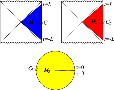
Figure 5: The bulk geometry $M=M_{1}+M_{2}+M_{3}$ that “fills in” the boundary contour $C=C_{1}+C_{2}+C_{3}$. For $d>3$, the Penrose diagrams for the Lorentzian patches drawn above are not accurate because the zigzag singularity lines must actually be not horizontal but bent inwards [67].

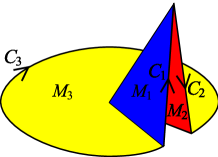
Figure 6: How to patch together the bulk patches $M_{1},M_{2},M_{3}$.

The way that three patches $M_{1,2,3}$ are glued together is simply the bulk extension of the way that the contours $C_{1,2,3}$ are glued together; see Figure 6.

Because now our spacetime is not just $M_{1}$ but $M=M_{1}+M_{2}+M_{3}$, the action have contributions from all of $M_{1,2,3}$, just as the boundary (4.14). Therefore, the bulk integration appearing e.g. in (D.46) should be now over all $M_{i}$, with the signs correctly taken into account:

$$G^{F}(\omega_{1},\omega_{2},\omega_{3},\omega_{4})=2\pi\kappa\delta(\omega_{1}+\omega_{2}+\omega_{3}+\omega_{4})$$

$$\times\biggl{\{}{1\over 4}\sum_{\text{perm}\atop(ijkl)}\int^{r}_{r_{H}}dr\biggl{[}\left({\omega_{i}\omega_{j}K_{[11]i}K_{[11]j}\over h}+{r^{4}h}K^{\prime}_{[11]i}K^{\prime}_{[11]j}\right)\left({\omega_{k}\omega_{l}K_{[11]k}K_{[11]l}\over h}+{r^{4}h}K^{\prime}_{[11]k}K^{\prime}_{[11]l}\right)$$

$$\qquad\qquad\qquad\quad-\left({\omega_{i}\omega_{j}K_{[21]i}K_{[21]j}\over h}+{r^{4}h}K^{\prime}_{[21]i}K^{\prime}_{[21]j}\right)\left({\omega_{k}\omega_{l}K_{[21]k}K_{[21]l}\over h}+{r^{4}h}K^{\prime}_{[21]k}K^{\prime}_{[21]l}\right)\biggr{]}$$

$$\qquad-6r\omega_{1}\omega_{2}\omega_{3}\omega_{4}\biggr{\}}.$$ (D.48)

Here, $K_{[ab]i}=K_{[ab]}(\omega_{i},r)$ and $K_{[ab]}(\omega,r)$ is the boundary-bulk propagator from the boundary $\partial M_{b}$ to the bulk $M_{a}$. The second line corresponds to the integration over $M_{1}$ and the third line to the integration over $M_{2}$. Because we are taking the $L\to\infty$ limit, the contribution from $M_{3}$ has been dropped. The counter term $-6r\omega_{1}\omega_{2}\omega_{3}\omega_{4}$ is added only for $M_{1}$, because the source is inserted only on $\partial M_{1}$ ($K_{[21]}(\omega,r)$ vanishes as $r\to\infty$).

Because the spacetime $M=M_{1}+M_{2}+M_{3}$ has no boundary inside, the boundary-bulk propagator can be determined without having to worry about boundary conditions. Carefully matching the values across different patches following [28, 29], we find the boundary-bulk propagators as follows:

$$\begin{split}K_{[11]}(\omega,r)&={1\over e^{\beta\omega}-1}[-\phi_{\omega}(r)+e^{\beta\omega}\phi_{-\omega}(r)],\\ \ K_{[21]}(\omega,r)&={e^{\beta\omega}\over e^{\beta\omega}-1}[-\phi_{\omega}(r)+\phi_{-\omega}(r)],\\ K_{[31]}(\omega,r)&={e^{(iL+\beta)\omega}\over e^{\beta\omega}-1}[-\phi_{\omega}(r)+\phi_{-\omega}(r)],\end{split}$$ (D.49)

where $\phi_{\pm\omega}(r)$ is the solution to the wave equation (D.25) satisfying the boundary condition (D.26). By substituting these propagators into (D.48), we can finally obtain the 4-point function for $F$.

D.4 Low frequency correlators

We are interested in the low frequency behavior of the correlation functions. As we discussed in Appendix B, the solution $\phi_{\pm\omega}(r)$ simplifies in the low frequency limit as

$$\phi_{\pm\omega}(r)\sim e^{\pm i\omega r_{*}}.$$ (D.50)

If we apply this to (D.48) and (D.49), we obtain the following low frequency behavior:

$$G^{F}(\omega_{1},\omega_{2},\omega_{3},\omega_{4}) \sim{\kappa\over\beta^{3}}\delta(\omega_{1}+\omega_{2}+\omega_{3}+\omega_{4})\sum\limits_{1\leq i<j\leq 4}(\omega_{i}+\omega_{j})\int_{-\infty}^{0}dr_{*}{r^{2}\over h}e^{-2i(\omega_{i}+\omega_{j})r_{*}}$$

$$\quad+\text{(higher powers in $\omega$)},$$ (D.51)

where we dropped numerical factors. Because we have rescaled $X$ in (D.5), to obtain the correlator for $F={\cal O}_{X}$ dual to the original $X$ before rescaling, we have to rescale $F\to{F\over\sqrt{2\pi{\alpha^{\prime}}}}$. Therefore, in the end, the 4-point function for $F$ is

$$G^{F}(\omega_{1},\omega_{2},\omega_{3},\omega_{4}) \sim{1\over{\alpha^{\prime}}\beta^{3}}\delta(\omega_{1}+\omega_{2}+\omega_{3}+\omega_{4})\sum\limits_{1\leq i<j\leq 4}(\omega_{i}+\omega_{j})\int_{-\infty}^{0}dr_{*}{r^{2}\over h}e^{-2i(\omega_{i}+\omega_{j})r_{*}}.$$ (D.52)

This is exactly the same as the result (4.21) that we obtained by a more naive method. Namely, this has exactly the same IR divergence as (4.21) that we studied in section 5.

D.5 Retarded 4-point function

In the above, we computed the time-ordered 4-point function for the force $F$ which turned out to be IR divergence. We can also compute the retarded 4-point function using the above formalism. As was shown in [29], for computing retarded correlators, one uses purely ingoing boundary condition for the boundary-bulk propagator:

$$K_{\text{ret}}(\omega,r)=\phi_{-\omega}(r).$$ (D.53)

If we define

$$G^{F}_{\text{ret}}(t_{1},t_{2},t_{3},t_{4})=\sum_{\text{perm}\atop(ijkl)}\theta(t_{i}>t_{j}>t_{k}>t_{l}){\langle{[[[F(t_{i}),F(t_{j})],F(t_{k})],F(t_{l})]}\rangle}$$ (D.54)

then the prescription of [29] gives

$$G^{F}_{\text{ret}}(\omega_{1},\omega_{2},\omega_{3},\omega_{4})=2\pi\kappa\delta(\omega_{1}+\omega_{2}+\omega_{3}+\omega_{4})$$

$$\times\biggl{\{}{1\over 4}\sum_{\text{perm}\atop(ijkl)}\int^{r}_{r_{H}}dr\left(\omega_{i}\omega_{j}K_{\text{ret},i}K_{\text{ret},j}+{r^{4}h}K^{\prime}_{\text{ret},i}K^{\prime}_{\text{ret},j}\right)\left(\omega_{k}\omega_{l}K_{\text{ret},k}K_{\text{ret},l}+{r^{4}h}K^{\prime}_{\text{ret},k}K^{\prime}_{\text{ret},l}\right)$$

$$\qquad-6r\omega_{1}\omega_{2}\omega_{3}\omega_{4}\biggr{\}},$$ (D.55)

where $K_{\text{ret},i}=K_{\text{ret}}(\omega_{i},r)$. The integration effectively becomes only over $M_{1}$.

For definiteness, consider the AdS₃ case where the retarded correlator is

$$K_{ret}(\omega,r)=\left(1-{i\omega\over r}\right)\left({r-r_{H}\over r+r_{H}}\right)^{-i\omega/2r_{H}}.$$ (D.56)

For this case, Eq. (D.55) gives

$$G^{F}_{\text{ret}}(\omega_{1},\omega_{2},\omega_{3},\omega_{4}) =\kappa 2\pi\delta(\omega_{1}+\cdots+\omega_{4})\,\omega_{1}\omega_{2}\omega_{3}\omega_{4}\left(2r_{H}-{16\sum_{i<j}\omega_{i}\omega_{j}\over r_{H}}\right).$$ (D.57)

Note that this is exact; we have not done low frequency approximation. This is both IR and UV finite.

Appendix E Computation of $\eta$ for the STU black hole

In this Appendix, we will compute the mean-free-path time for the STU black hole studied in 6.2. The final results have been presented in (6.40) and (6.41)–(6.2.4).

We will discuss the 1-charge case ($\kappa_{1}=\kappa,\kappa_{2}=\kappa_{3}=0$) only, because the 2- and 3-charge cases are similar. First, the relations (6.20), (6.21), and (6.22) read, in this case,

$$m={r_{H}^{4}\over l^{2}}(1+\kappa),\qquad T={r_{H}\over 2\pi}{2+\kappa\over\sqrt{1+\kappa}},\qquad\Phi=-{r_{H}^{2}\over\kappa_{5}^{2}l}\sqrt{\kappa}.$$ (E.1)

$L_{H}$ in (6.40) can be computed as follows. From the definition (6.13) and (6.39) for $n=1$, we obtain

$$\int_{\infty}^{r}dr{H^{1/2}\over r^{2}f}{1\over\sqrt{1-f^{-1}H^{2}{\cal A}_{t}^{2}}} =\int_{\infty}^{r}{dr\over r^{2}-r_{H}^{2}}\sqrt{r_{H}^{2}+\ell^{2}\over(r^{2}+r_{H}^{2}+\ell^{2})((r_{H}^{2}+\ell^{2})r^{2}+r_{H}^{4})}.$$

$$={1\over 2r_{H}^{3}}{\sqrt{1+\kappa}\over(2+\kappa)}\log{r-r_{H}\over L_{H}}+{\cal O}(r-r_{H})$$ (E.2)

The integral in the first line diverges as $r\to r_{H}$. We can separate this divergent piece by subtracting and adding the term obtained by setting $r$ to $r_{H}$ in the square root. Further setting $\rho=r/r_{H}$ and $\kappa=\ell^{2}/r_{H}$, we have

$${1\over 2r_{H}^{3}}{\sqrt{1+\kappa}\over(2+\kappa)}\left\{\log{r-r_{H}\over r+r_{H}}+2(2+\kappa)\int_{\infty}^{1}{d\rho\over\rho^{2}-1}\left[{1\over\sqrt{(\rho+1+\kappa)((1+\kappa)\rho^{2}+1)}}-{1\over(2+\kappa)}\right]\right\}$$

$$\equiv{1\over 2r_{H}^{3}}{\sqrt{1+\kappa}\over(2+\kappa)}\log{r-r_{H}\over L_{H}}+{\cal O}(r-r_{H}).$$ (E.3)

In the second term in the first line, we have set the upper limit of the integral to $\rho\to 1$ (which is equivalent to $r\to r_{H}$) because the integral is now convergent. By comparing both sides, we obtain

$$L_{H}=2r_{H}\exp\left\{-2(2+\kappa)\int_{\infty}^{1}{d\rho\over\rho^{2}-1}\left[{1\over\sqrt{(\rho^{2}+1+\kappa)((1+\kappa)\rho^{2}+1)}}-{1\over 2+\kappa}\right]\right\}.$$ (E.4)

By using (E.1), we obtain the final expression (6.41). For small $\kappa$, it is easy to expand the integrand in (6.41) in $\kappa$, and each integral converges. This leads to the following expansion of $\eta$ in $\kappa$:

$$\eta=e^{-\pi/2}\left[2\pi-\pi\kappa+\frac{(12-\pi)\pi}{16}\kappa^{2}\right]+{\cal O}\left(\kappa^{3}\right)$$ (E.5)

This shows that, as $\kappa$ increases with fixed $T$, the mean-free-path time $t_{mfp}$ increases.

The 2- and 3-charge cases are similar and we obtain (6.42) and (6.2.4). The small $\kappa$ expansion of $\eta$ is

$$\eta =e^{-\pi/2}\left[2\pi-\frac{1}{2}(4-\pi)\pi\kappa+\frac{1}{16}\pi\left(52-19\pi+\pi^{2}\right)\kappa^{2}+O\left(\kappa^{3}\right)\right]$$ (E.6)

$$\eta =e^{-\pi/2}\left[2\pi+(\pi-3)\pi\kappa+\frac{1}{16}\pi\left(140-57\pi+4\pi^{2}\right)\kappa^{2}+O\left(\kappa^{3}\right)\right]$$ (E.7)

for the 2- and 3-charge cases, respectively.

References

- [1] R. Brown, “A brief account of microscopical observations made in the months of June, July and August, 1827, on the particles contained in the pollen of plants; and on the general existence of active molecules in organic and inorganic bodies,” Philos. Mag. 4, 161 (1828); reprinted in Edinburgh New Philos. J. 5, 358 (1928).
- [2] G. E. Uhlenbeck and L. S. Ornstein, “On The Theory Of The Brownian Motion,” Phys. Rev. 36, 823 (1930); S. Chandrasekhar, “Stochastic problems in physics and astronomy,” Rev. Mod. Phys. 15, 1 (1943); M. C. Wang and G. E. Uhlenbeck, “On the Theory of the Brownian Motion II,” Rev. Mod. Phys. 17, 323 (1945).
- [3] B. Duplantier, “Brownian Motion, ‘Diverse and Undulating’,” in “Einstein, 1905-2005,” Poincaré Seminar 2005, Th. Damour, O. Darrigol, B. Duplantier and V. Rivasseau, Eds., pp. 201-293 (Birkhäuser Verlag, Basel, 2006) [arXiv:0705.1951 [cond-mat.stat-mech]].
- [4] J. M. Maldacena, “The large N limit of superconformal field theories and supergravity,” Adv. Theor. Math. Phys. 2 (1998) 231 [Int. J. Theor. Phys. 38 (1999) 1113] [arXiv:hep-th/9711200].
- [5] S. S. Gubser, I. R. Klebanov and A. M. Polyakov, “Gauge theory correlators from non-critical string theory,” Phys. Lett. B 428, 105 (1998) [arXiv:hep-th/9802109].
- [6] E. Witten, “Anti-de Sitter space and holography,” Adv. Theor. Math. Phys. 2, 253 (1998) [arXiv:hep-th/9802150].
- [7] P. Kovtun, D. T. Son and A. O. Starinets, “Viscosity in strongly interacting quantum field theories from black hole physics,” Phys. Rev. Lett. 94, 111601 (2005) [arXiv:hep-th/0405231].
- [8] C. P. Herzog, A. Karch, P. Kovtun, C. Kozcaz and L. G. Yaffe, “Energy loss of a heavy quark moving through N = 4 supersymmetric Yang-Mills plasma,” JHEP 0607, 013 (2006) [arXiv:hep-th/0605158].
- [9] H. Liu, K. Rajagopal and U. A. Wiedemann, “Calculating the jet quenching parameter from AdS/CFT,” Phys. Rev. Lett. 97, 182301 (2006) [arXiv:hep-ph/0605178].
- [10] S. S. Gubser, “Drag force in AdS/CFT,” Phys. Rev. D 74, 126005 (2006) [arXiv:hep-th/0605182].
- [11] C. P. Herzog, “Energy loss of heavy quarks from asymptotically AdS geometries,” JHEP 0609, 032 (2006) [arXiv:hep-th/0605191].
- [12] J. Casalderrey-Solana and D. Teaney, “Heavy quark diffusion in strongly coupled N = 4 Yang Mills,” Phys. Rev. D 74, 085012 (2006) [arXiv:hep-ph/0605199].
- [13] S. S. Gubser, “Momentum fluctuations of heavy quarks in the gauge-string duality,” Nucl. Phys. B 790, 175 (2008) [arXiv:hep-th/0612143].
- [14] H. Liu, K. Rajagopal and U. A. Wiedemann, “Wilson loops in heavy ion collisions and their calculation in AdS/CFT,” JHEP 0703, 066 (2007) [arXiv:hep-ph/0612168].
- [15] J. Casalderrey-Solana and D. Teaney, “Transverse momentum broadening of a fast quark in a N = 4 Yang Mills plasma,” JHEP 0704, 039 (2007) [arXiv:hep-th/0701123].
- [16] S. Bhattacharyya, V. E. Hubeny, S. Minwalla and M. Rangamani, “Nonlinear Fluid Dynamics from Gravity,” JHEP 0802, 045 (2008) [arXiv:0712.2456 [hep-th]].
- [17] D. T. Son and A. O. Starinets, “Viscosity, Black Holes, and Quantum Field Theory,” Ann. Rev. Nucl. Part. Sci. 57, 95 (2007) [arXiv:0704.0240 [hep-th]].
- [18] A. E. Lawrence and E. J. Martinec, “Black Hole Evaporation Along Macroscopic Strings,” Phys. Rev. D 50, 2680 (1994) [arXiv:hep-th/9312127].
- [19] S. J. Rey and J. T. Yee, “Macroscopic strings as heavy quarks in large N gauge theory and anti-de Sitter supergravity,” Eur. Phys. J. C 22, 379 (2001) [arXiv:hep-th/9803001].
- [20] R. C. Myers, A. O. Starinets and R. M. Thomson, “Holographic spectral functions and diffusion constants for fundamental matter,” JHEP 0711, 091 (2007) [arXiv:0706.0162 [hep-th]].
- [21] J. de Boer, V. E. Hubeny, M. Rangamani and M. Shigemori, “Brownian motion in AdS/CFT,” JHEP 0907, 094 (2009) [arXiv:0812.5112 [hep-th]].
- [22] D. T. Son and D. Teaney, “Thermal Noise and Stochastic Strings in AdS/CFT,” JHEP 0907, 021 (2009) [arXiv:0901.2338 [hep-th]].
- [23] G. C. Giecold, E. Iancu and A. H. Mueller, “Stochastic trailing string and Langevin dynamics from AdS/CFT,” JHEP 0907, 033 (2009) [arXiv:0903.1840 [hep-th]].
- [24] G. C. Giecold, “Heavy quark in an expanding plasma in AdS/CFT,” JHEP 0906, 002 (2009) [arXiv:0904.1874 [hep-th]].
- [25] J. Casalderrey-Solana, K. Y. Kim and D. Teaney, “Stochastic String Motion Above and Below the World Sheet Horizon,” JHEP 0912, 066 (2009) [arXiv:0908.1470 [hep-th]].
- [26] U. Gursoy, E. Kiritsis, L. Mazzanti and F. Nitti, “Langevin diffusion of heavy quarks in non-conformal holographic backgrounds,” JHEP 1012, 088 (2010) [arXiv:1006.3261 [hep-th]].
- [27] K. Skenderis, “Lecture notes on holographic renormalization,” Class. Quant. Grav. 19, 5849 (2002) [arXiv:hep-th/0209067].
- [28] K. Skenderis and B. C. van Rees, “Real-time gauge/gravity duality: Prescription, Renormalization and Examples,” JHEP 0905, 085 (2009) [arXiv:0812.2909 [hep-th]].
- [29] B. C. van Rees, “Real-time gauge/gravity duality and ingoing boundary conditions,” Nucl. Phys. Proc. Suppl. 192-193, 193 (2009) [arXiv:0902.4010 [hep-th]].
- [30] R. Kubo, “The fluctuation-dissipation theorem,” Rep. Prog. Phys. 29, 255-284 (1966).
- [31] H. Mori, “Transport, collective motion, and Brownian motion,” Prog. Theor. Phys. 33, 423 (1965).
- [32] R. Kubo, M. Toda, and N. Hashitsume, “Statistical Physics II – Nonequilibrium Statistical Mechanics,” Springer-Verlag.
- [33] F. Dominguez, C. Marquet, A. H. Mueller, B. Wu and B. W. Xiao, “Comparing energy loss and -broadening in perturbative QCD with strong coupling SYM theory,” Nucl. Phys. A 811, 197 (2008) [arXiv:0803.3234 [nucl-th]].
- [34] G. Beuf, C. Marquet and B. W. Xiao, “Heavy-quark energy loss and thermalization in a strongly coupled SYM plasma,” Phys. Rev. D 80, 085001 (2009) [arXiv:0812.1051 [hep-ph]].
- [35] M. Chernicoff, J. A. Garcia and A. Guijosa, “A Tail of a Quark in N=4 SYM,” JHEP 0909, 080 (2009) [arXiv:0906.1592 [hep-th]].
- [36] V. Balasubramanian, P. Kraus and A. E. Lawrence, “Bulk vs. boundary dynamics in anti-de Sitter spacetime,” Phys. Rev. D 59, 046003 (1999) [arXiv:hep-th/9805171].
- [37] N. D. Birrell and P. C. W. Davies, “Quantum Fields In Curved Space,” Cambridge, UK: Univ. Pr. (1982) 340p
- [38] K. Behrndt, M. Cvetic and W. A. Sabra, “Non-extreme black holes of five dimensional N = 2 AdS supergravity,” Nucl. Phys. B 553, 317 (1999) [arXiv:hep-th/9810227].
- [39] M. Cvetic et al., “Embedding AdS black holes in ten and eleven dimensions,” Nucl. Phys. B 558, 96 (1999) [arXiv:hep-th/9903214].
- [40] P. Kraus, F. Larsen and S. P. Trivedi, “The Coulomb branch of gauge theory from rotating branes,” JHEP 9903, 003 (1999) [arXiv:hep-th/9811120].
- [41] J. G. Russo and K. Sfetsos, “Rotating D3 branes and QCD in three dimensions,” Adv. Theor. Math. Phys. 3, 131 (1999) [arXiv:hep-th/9901056].
- [42] E. Caceres and A. Guijosa, “Drag force in charged N = 4 SYM plasma,” JHEP 0611, 077 (2006) [arXiv:hep-th/0605235].
- [43] C. P. Herzog and A. Vuorinen, “Spinning Dragging Strings,” JHEP 0710, 087 (2007) [arXiv:0708.0609 [hep-th]].
- [44] T. Harmark, J. Natario and R. Schiappa, “Greybody Factors for d-Dimensional Black Holes,” Adv. Theor. Math. Phys. 14, 727 (2010) [arXiv:0708.0017 [hep-th]].
- [45] J. Dunkel and P. Hänggi, “Relativistic Brownian Motion,” Phys. Rep. 471, 1 (2009) [arXiv:0812.1996 [cond-mat]].
- [46] P. Hänggi, P. Talkner and M. Borkovec, “Reaction-rate theory: fifty years after Kramers,” Rev. Mod. Phys. 62, 251 (1990).
- [47] A.A. Dubkov, P. Hänggi, and I. Goychuk, “Non-linear Brownian motion: the problem of obtaining the thermal Langevin equation for a non-Gaussian bath,” J. Stat. Mech. P01034 (2009).
- [48] G. F. Efremov “A Fluctuation Dissipation Theorem for Nonlinear Media,” Sov. Phys. JETP 28, 1232 (1969); M. S. Gupta, “Thermal fluctuations in driven nonlinear resistive systems,” Phys. Rev. A 18, 2725 (1978); M. G. Gupta, “Thermal Noise in Nonlinear Resistive Devices and Its Circuit Representation,” Proc. IEEE 70, 788 (1982); G. N. Bochkov, Yu. E. Kuzovlev, “Nonlinear fluctuation-dissipation relations and stochastic models in nonequilibrium thermodynamics : I. Generalized fluctuation-dissipation theorem,” Physica A 106, 443 (1981); E. Wang and U. Heinz, “Generalized fluctuation-dissipation theorem for nonlinear response functions,” Phys. Rev. D 66, 025008 (2002)
- [49] M. Le Bellac, “Thermal Field Theory,” Cambridge, UK: Univ. Pr. (1996)
- [50] K.-c. Chou, Z.-b. Su, B.-l. Hao and L. Yu, “Equilibrium and Nonequilibrium Formalisms Made Unified,” Phys. Rept. 118, 1 (1985).
- [51] P. Aurenche and T. Becherrawy, “A Comparison of the real time and the imaginary time formalisms of finite temperature field theory for 2, 3, and 4 point Green’s functions,” Nucl. Phys. B 379, 259 (1992).
- [52] P. Aurenche, T. Becherrawy and E. Petitgirard, “Retarded / advanced correlation functions and soft photon production in the hard loop approximation,” hep-ph/9403320.
- [53] F. L. Lin and T. Matsuo, “Jet quenching parameter in medium with chemical potential from AdS/CFT,” Phys. Lett. B 641, 45 (2006) [arXiv:hep-th/0606136].
- [54] S. D. Avramis and K. Sfetsos, “Supergravity and the jet quenching parameter in the presence of R-charge densities,” JHEP 0701, 065 (2007) [arXiv:hep-th/0606190].
- [55] N. Armesto, J. D. Edelstein and J. Mas, “Jet quenching at finite ’t Hooft coupling and chemical potential from AdS/CFT,” JHEP 0609, 039 (2006) [arXiv:hep-ph/0606245].
- [56] E. Caceres, M. Natsuume and T. Okamura, “Screening length in plasma winds,” JHEP 0610, 011 (2006) [arXiv:hep-th/0607233].
- [57] S. D. Avramis, K. Sfetsos and D. Zoakos, “On the velocity and chemical-potential dependence of the heavy-quark interaction in N = 4 SYM plasmas,” Phys. Rev. D 75, 025009 (2007) [arXiv:hep-th/0609079].
- [58] K. Maeda, M. Natsuume and T. Okamura, “Dynamic critical phenomena in the AdS/CFT duality,” Phys. Rev. D 78, 106007 (2008) [arXiv:0809.4074 [hep-th]].
- [59] J. Mas, “Shear viscosity from R-charged AdS black holes,” JHEP 0603, 016 (2006) [arXiv:hep-th/0601144].
- [60] M. Cvetic and S. S. Gubser, “Thermodynamic Stability and Phases of General Spinning Branes,” JHEP 9907, 010 (1999) [arXiv:hep-th/9903132].
- [61] S. Bhattacharyya, S. Lahiri, R. Loganayagam and S. Minwalla, “Large rotating AdS black holes from fluid mechanics,” JHEP 0809, 054 (2008) [arXiv:0708.1770 [hep-th]].
- [62] P. Hayden and J. Preskill, “Black holes as mirrors: quantum information in random subsystems,” JHEP 0709, 120 (2007) [arXiv:0708.4025 [hep-th]].
- [63] Y. Sekino and L. Susskind, “Fast Scramblers,” JHEP 0810, 065 (2008) [arXiv:0808.2096 [hep-th]].
- [64] M. E. Carrington, T. Fugleberg, D. S. Irvine and D. Pickering, “Real time statistical field theory,” Eur. Phys. J. C 50, 711 (2007) [arXiv:hep-ph/0608298].
- [65] P. Arnold and L. G. Yaffe, “Effective theories for real-time correlations in hot plasmas,” Phys. Rev. D 57, 1178 (1998) [arXiv:hep-ph/9709449].
- [66] N. Iqbal and H. Liu, “Universality of the hydrodynamic limit in AdS/CFT and the membrane paradigm,” Phys. Rev. D 79, 025023 (2009) [arXiv:0809.3808 [hep-th]].
- [67] L. Fidkowski, V. Hubeny, M. Kleban and S. Shenker, “The black hole singularity in AdS/CFT,” JHEP 0402, 014 (2004) [arXiv:hep-th/0306170].