Surface tensions, surface potentials and the Hofmeister series of electrolyte solutions

Abstract

A theory is presented which allows us to accurately calculate the surface tensions and the surface potentials of electrolyte solutions. Both the ionic hydration and the polarizability are taken into account. We find a good correlation between the Jones-Dole viscosity $B$-coefficient and the ionic hydration near the air-water interface. The kosmotropic anions such as fluoride, iodate, sulfate and carbonate, are found to be strongly hydrated and are repelled from the interface. The chaotropic anions such as perchlorate, iodide, chlorate and bromide are found to be significantly adsorbed to the interface. Chloride and bromate anions become weakly hydrated in the interfacial region. The sequence of surface tensions and surface potentials is found to follow the Hofmeister ordering. The theory, with only one adjustable parameter, quantitatively accounts for the surface tensions of 10 sodium salts for which there is experimental data.

Universidade Federal do Rio Grande do Sul] Instituto de Física, Universidade Federal do Rio Grande do Sul, Caixa Postal 15051, CEP 91501-970, Porto Alegre, RS, Brazil Universidade Federal de Pelotas] Departamento de Física, Instituto de Física e Matemática, Universidade Federal de Pelotas, Caixa Postal 354, CEP 96010-900, Pelotas, RS, Brazil Universidade Federal do Rio Grande do Sul] Instituto de Física, Universidade Federal do Rio Grande do Sul, Caixa Postal 15051, CEP 91501-970, Porto Alegre, RS, Brazil

1 Introduction

Electrolyte solutions have been the subject of intense study for over a century. While the bulk properties of electrolytes are now quite well understood, their behavior at interfaces and surfaces still remains a puzzle. Over a hundred years ago, Hofmeister observed that presence of electrolyte in water modified significantly solubility of proteins. While some salts lead to protein precipitation (salting out), other salts stabilize proteins increasing their solubility (salting in). A few years after this curious observation, Heydweiller ¹ discovered that salt dissolved in water increased the surface tension of solution-air interface. While cations had only a small influence on the surface tension, anions affected it quite significantly. Furthermore, the magnitude of the variation of the surface tension followed the same sequence discovered by Hofmeister earlier. It appeared that the two effects were related.

Because of its great importance for biology, over the last century there has been a tremendous effort to understand the ionic specificity. Since air-water interface is relative simple, as compared to proteins, most of the theoretical work has concentrated on it. Langmuir ² was the first to attempt a theoretical explanation of the physical mechanism behind the increase of the surface tension produced by electrolytes. Using the Gibbs adsorption isotherm equation, Langmuir concluded that the phenomenon was a consequence of ion depletion near the air-water interface, and suggested that the depleted layer was about $4$ Å in width. No clear explanation for existence of this ion-free layer was provided by Langmuir, and soon it became clear that in order to obtain a reasonable agreement with experiments, its width had to be a function of ionic concentration ^{3, *HaGi26}. A further insight was provided by Wagner ⁵, based on the Debye-Hückel (DH) theory of strong electrolytes ⁶. Wagner argued that ionic depletion was a consequence of the electrostatic repulsion produced by the interaction of ions with their electrostatic images across the air-water interface. Wagner’s theory was quite complicated and a simplified version was proposed by Onsager and Samaras (OS), who also derived a limiting law which, they argued, had a universal validity for all electrolytes at sufficiently low concentrations ⁷. Indeed, careful experimental measurements have confirmed the OS limiting law ^{8, *Pa59}. However at larger concentrations, OS theory was found to strongly underestimate surface tensions.

Similar to Langmuir, Wagner and OS integrated the Gibbs adsorption isotherm equation to obtain the excess surface tension. Some time ago, Levin and Flores-Mena (LFM) proposed a different approach based on the direct Helmholtz free energy calculation ¹⁰. The LFM theory combined Langmuir, Wagner, and OS insights into one theory. They argued that in addition to the ion-image interaction, ionic hydration leads to a hard-core-like repulsion from the Gibbs dividing surface. Using a $2$ Å hydrated radius of Na+ and Cl-, they were able to obtain a very good agreement with the experimental measurements of surface tension of NaCl solution, up to $1$ M concentration. However, the LFM theory failed to correctly account for the ionic specificity, predicting that the surface tension of NaI salt should be larger than that of NaCl, contrary to experiments. It was clear that the LFM theory was still lacking an important ingredient. An indication of the missing ingredient was already present in the work of Frumkin, 80 years earlier ¹¹. Frumkin measured the electrostatic potential difference across the solution-air interface and found that for all halogen salts, except fluoride, potential was lower in air than in water. This meant that anions were preferentially solvated near the interface. Boström et al. ¹² suggested that this ionic specificity, was a consequence of dispersion forces arising from finite frequency electromagnetic fluctuations. Their theory, however, predicted surface potentials of opposite sign to the ones measured by Frumkin, implying that cations were preferentially adsorbed to the interface. This was clearly contradicted by the simulations on small water clusters ^{13, *DaSm93, *StBr99}, as well as by the subsequent large scale polarizable force fields simulations ^{16, *JuTo06, *HoNe07, *Br08} and by the photoelectron emission experiments ^{20, *Gh05, *Ga04}. All these agreed with Frumkin that large anions, and not small cations, that are preferentially solvated near the air-water interface. A theoretical explanation for this behavior was advanced by Levin ²³, who argued that anionic surface solvation was a consequence of the competition between the cavitational and the electrostatic energies. The cavitational energy arises from the perturbation to the hydrogen bond network produced by ionic solvation. This results in a short range force which drives ions towards the interface. This is counterbalanced by the electrostatic Born solvation force which arises from the dipolar screening of the ionic self-energy in aqueous environment. For hard (weakly polarizable) ions, the Born energy is much larger than the cavitational energy, favoring the bulk solvation. However for large polarizable ions, the energy balance is shifted. For such ions, ionic charge can easily redistribute itself so that even if a large fraction of ionic volume is exposed to air, the electrostatic energy penalty for this remains small, since most of the ionic charge remains hydrated. This means that through surface solvation, large, strongly polarizable ions, can have the best of two worlds — gain the cavitational energy at a small price in electrostatic self energy. Levin derived the interaction potential quantifying this effect ²³. In a follow up paper, Levin et al. ²⁴ used this potential to quantitatively account for the surface tensions of all sodium-halide salts. In this paper we will extend the theory of reference ²⁴ to calculate the surface tensions and the surface potentials of others sodium salts and to derive the Hofmeister series.

2 Model and theory

Consider an electrolyte solution confined to a mesoscopic drop of water of radius $R$, which corresponds to the position of the Gibbs dividing surface (GDS) ^{25, 24}. We define the adsorption (ion excess per unit area) as

$$\Gamma_{\pm}=\frac{1}{4\pi R^{2}}\left[\int_{0}^{\infty}\rho_{\pm}(r)4\pi r^{2}{\rm d}r-\frac{4\pi R^{3}}{3}c_{b}\right]\ ,$$ (1)

where $\rho_{\pm}(r)$ are the ionic density profiles and $c_{b}=\rho_{+}(0)=\rho_{-}(0)$ is the bulk concentration of electrolyte. If $N$ ion pairs are inside the drop, eq 1 simplifies to $\Gamma\pm=N/4\pi R^{2}-c_{b}R/3$.

The water and air will be treated as uniform dielectrics of permittivities $\epsilon_{w}=80$ and $\epsilon_{a}=1$, respectively. The surface tension can be obtained by integrating the Gibbs adsorption isotherm equation, ${\rm d}\gamma=-\Gamma_{+}{\rm d}\mu_{+}-\Gamma_{-}{\rm d}\mu_{-}$, where $\beta\mu_{\pm}=\ln(c_{b}\Lambda_{\pm}^{3})$ are the chemical potentials and $\Lambda_{\pm}$ are the de Broglie thermal wavelengths. Let us first consider alkali-metal cations, such as lithium, sodium, or potassium. Because these cations are small, they have large surface charge density, which leads to strong interaction with surrounding water molecules, resulting in an effective hydrated radius $a_{h}$. We can, therefore, model these ions as hard spheres of radius $a_{h}$ with a point charge $q$ located at the origin. Because of their strong hydration, these cations can not move across the GDS since this would require them to shed their solvation sheath. For mesoscopic drops we can neglect the curvature of the GDS. To bring a cation from bulk electrolyte to some distance $z>a_{h}$ from the GDS then requires ^{10, 24}

$$W(z;a_{h})=\frac{q^{2}}{2\epsilon_{w}}\int_{0}^{\infty}dke^{-2s(z-a_{h})}\frac{k[s\cosh(ka_{h})-k\sinh(ka_{h})]}{s[s\cosh(ka_{h})+k\sinh(ka_{h})]}\ ,$$ (2)

of work. The GDS is located at $z=0$ and the axis is oriented into the drop. We have defined $s=\sqrt{\kappa^{2}+k^{2}}$, where $\kappa=\sqrt{8\pi q^{2}c_{b}/\epsilon_{w}k_{B}T}$ is the inverse Debye length. The eq 2 is well approximated by

$$W_{ap}(z;a_{h})=\frac{W(a_{h};a_{h})a_{h}}{z}\ e^{-2\kappa(z-a_{h})}\,,$$ (3)

see 1. This form will be used later to speed up the numerical calculations.

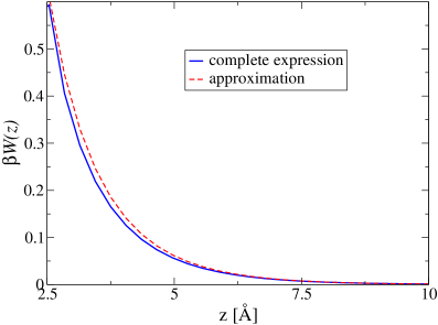
Figure 1: Comparison between the complete expression (eq 2) and its approximation (eq 3), for an ion of radius $2.5$ Åat 1M concentration.

Unlike small cation, large halogen anions of bare radius $a_{0}$ have low electronic charge density and are weakly hydrated. The polarizability of an anion is $\gamma_{a}$ and we define its relative polarizability as $\alpha=\gamma_{a}/a_{0}^{3}$. We can model these ions as imperfect spherical conductors. When an anion is far from the interface, its charge $-q$ is uniformly distributed over its surface. However, when an anion begins to cross the GDS, its charge starts to redistribute itself on the surface so as to leave most of it in the high dielectric environment ²³. The fraction of charge $x$ which remains hydrated when the ionic center is at distance $z$ from the GDS is determined by the minimization of the polarization energy ²³,

$$U_{p}(z,x)=\frac{q^{2}}{2a_{0}\epsilon_{w}}\left[\frac{\pi x^{2}}{\theta(z)}+\frac{\pi[1-x]^{2}\epsilon_{w}}{[\pi-\theta(z)]\epsilon_{o}}\right]+\frac{g}{\beta}\left[x-\frac{1-cos[\theta(z)]}{2}\right]^{2}\ ,$$ (4)

where $\theta(z)=\arccos[-z/a_{0}]$ and $g=(1-\alpha)/\alpha$. We find

$$x(z)=\left[\frac{\lambda_{B}\pi\epsilon_{w}}{a_{0}\epsilon_{o}\left[\pi-\theta(z)\right]}+g[1-cos[\theta(z)]]\right]/\left[\frac{\lambda_{B}\pi}{a_{0}\theta(z)}+\frac{\lambda_{B}\pi\epsilon_{w}}{a_{0}\epsilon_{0}[\pi-\theta(z)]}+2g\right]\ .$$ (5)

Substituting this back into eq 4, we obtain the polarization potential. This potential is repulsive, favoring ions to move towards the bulk. Nevertheless, the repulsion is quite soft compared to a hard-core-like repulsion of strongly hydrated cations. The force that drives anions toward the interface arises from cavitation. When ion is dissolved in water it creates a cavity from which water molecules are expelled. This leads to a perturbation to the hydrogen bond network and an energetic cost. For small voids, the cavitational energy scales with their volume. ^{26, *Ch05}. As an ion moves across the interface, the cavity that it creates in water diminishes proportionally to the fraction of the volume exposed to air ^{23, 24}, producing a short-range interaction potential that forces ions to move across the GDS,

$$U_{cav}(z)=\left\{\begin{array}[]{l}\nu a_{0}^{3}\text{ for }z\geq a_{0}\ ,\\ \frac{1}{4}\nu a_{0}^{3}\left(\frac{z}{a_{0}}+1\right)^{2}\left(2-\frac{z}{a_{0}}\right)\text{ for }-a_{0}<z<a_{0}\ ,\end{array}\right.$$ (8)

where $\nu\approx 0.3k_{B}T/$ ų is obtained from bulk simulations ²⁸. For small strongly hydrated cations, this energy gain does not compensate for the electrostatic energy penalty of exposing ionic charge to the low dielectric environment. For large polarizable ions, on the other hand, electrostatic energy penalty is small, and the cavitational energy is sufficient to favor the surface solvation. The total potential felt by an unhydrated anion is then ²⁴

$$U_{tot}(z)=\left\{\begin{array}[]{l}W(z;a_{0})+\nu a_{0}^{3}+\frac{q^{2}}{2\epsilon_{w}a_{0}}\,\text{ for }z\geq a_{0}\ ,\\ W(a_{0};a_{0})z/a_{0}+U_{p}(z)+U_{cav}(z)\,\text{ for }0<z<a_{0}\ ,\\ U_{p}(z)+U_{cav}(z)\,\text{ for }-a_{0}<z\leq 0\ .\end{array}\right.$$ (12)

The density profiles can now be calculated by integrating the non-linear modified Poisson-Boltzmann equation (mPB):

$$\nabla^{2}\phi(r) = -\frac{4\pi q}{\epsilon_{w}}\left[\rho_{+}(r)-\rho_{-}(r)\right]\ ,$$

$$\rho_{+}(r) = \frac{N\Theta(R-a_{h}-r)e^{-\beta q\phi(r)-\beta W(z;a_{h})}}{\int_{0}^{R-a_{h}}4\pi r^{2}\,dr\,e^{-\beta q\phi(r)-\beta W(z;a_{h})}}\ ,$$ (13)

$$\rho_{-}(r) = \frac{Ne^{\beta q\phi(r)-\beta U_{tot}(r)}}{\int_{0}^{R+a_{0}}4\pi r^{2}\,dr\,e^{\beta q\phi(r)-\beta U_{tot}(r)}}\ ,$$

where $\Theta$ is the Heaviside step function. To speed up the numerical calculations we can replace $W\rightarrow W_{ap}$.

3 Sodium-Halogen Salts

First, we study the sodium-halogen salts ²⁴. The anion radii were obtained by Latimer, Pitzer and Slansky ²⁹ by fitting the experimentally measured free energies of hydration to the Born model. Since our theory in the bulk also reduces to the Born model, these radii are particularly appropriate: $a_{I}=2.26$ Å, $a_{Br}=2.05$ Å, $a_{Cl}=1.91$ Å and $a_{F}=1.46$ Å. For ionic polarizabilities we use the values from the reference ³⁰: $\gamma_{I}=7.4$ ų, $\gamma_{Br}=5.07$ ų, $\gamma_{Cl}=3.77$ ų and $\gamma_{F}=1.31$ ų.

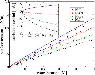
Figure 2: Surface tensions for NaF, NaCl, NaBr and NaI. The symbols are the experimental data ^{31, 32, 33} and the lines are the results of the present theory. The inset shows the surface potential difference as a function of molar concentration.

The excess surface tension can be obtained by integrating the Gibbs adsorption isotherm equation (eq 1). We start with NaI. Since I- is large and soft, it should be unhydrated in the interfacial region. Adjusting the hydrated radius of Na+ to best fit the experimental data ³¹ for NaI, we obtain ²⁴ $a_{h}=2.5$ Å. We will use this partially hydrated radius of Na+ in the rest of the paper. Considering that Br- is also large and soft, we expect that it will also remain unhydrated in the interfacial region. This expectation is well justified and we obtain a very good agreement with the experimental data ³³, see 2. For F- the situation should be very different. This ion is small, hard and strongly hydrated. This means that just like for a cation, a hard core repulsion from the GDS must be explicitly included in the mPB equation. For hydrated (or partially hydrated) anions the density is then

$$\rho_{-}(r) = \frac{N\Theta(R-a_{h}-r)e^{\beta q\phi(r)-\beta W(z;a_{h})}}{\int_{0}^{R-a_{h}}4\pi r^{2}\,dr\,e^{\beta q\phi(r)-\beta W(z;a_{h})}}\ ,$$ (14)

Using this in eq 2, an almost perfect agreement with the experimental data ³¹ is found for NaF, using the usual bulk hydrated radius of F-, $a_{h}=3.52$ ų⁴, see 2. The table salt, NaCl, is the most difficult case to study theoretically, since Cl- is sufficiently small to remain partially hydrated near the GDS. We find a good fit to the experimental data ³², 2, using a partially hydrated radius of Cl-, $a_{h}=2.0$ Å, which is very close to its bare size.

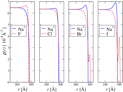
Figure 3: Theoretical ionic density profiles for NaF, NaCl, NaBr and NaI at $1$M. The GDS is at $r=300$ Å.

The ionic density profiles for these salts are plotted in 3. In agreement with the polarizable force fields simulations ^{13, *DaSm93, *StBr99, 16, *JuTo06, *HoNe07, *Br08}, the large halogens I- and Br- are strongly adsorbed at the interface. However, just as was found using the vibrational sum-frequency spectroscopy ³⁵, their concentration at the GDS remains below that in the bulk. The electrostatic potential difference across the air-water interface is $\chi=\phi(\infty)-\phi(0)$. We find that our theoretical values for the surface potentials are in reasonable agreement with the measurements of Frumkin ^{11, 36} and Jarvis et al. ³⁷, 1.

Table 1: Surface potentials difference at $1$ M for various salts

	Calculated (mV)	Frumkin 11, 36 (mV)	Jarvis et al. 37 (mV)
NaF	4.7	–	–
NaCl	-2.1	-1	$\approx$ -1
NaBr	-9.4	–	$\approx$ -5
NaI	-14.3	-39	$\approx$ -21
NaIO3	5	–	–
NaBrO3	-0.12	–	–
NaNO3	-8.27	-17	$\approx$ -8
NaClO3	-11.02	-41	–
NaClO4	-31.1	-57	–
Na2CO3	10.54	3	$\approx$ 6
Na2SO4	10.17	3	$\approx$ 35

4 Oxy-Anion Salts

We next study the surface potentials and the surface tensions of sodium salts with more complex anions, such as: chlorate, nitrate, bromate, iodate, perchlorate, sulfate and carbonate. Naively one might expect that because of their large size, these oxy-anions will loose their hydration near the GDS. This, however, is not necessarily the case. At the moment there is no reliable theory of hydration, nevertheless, it has been known for a long time that ions can be divided into two categories: structure-makers (kosmotropes) and structure-breakers (chaotropes). This dichotomy is reflected, for example, in the Jones-Dole viscosity $B$-coefficient. It is found experimentally that for large dilutions, viscosity varies with the concentration of electrolyte as ³⁸:

$$\eta_{r}=1+A\rho^{1/2}+B\rho\ ,$$ (15)

where $A$ is a positive constant, resulting from the ion-ion interactions; and $B$ is related to the ion-solvent interactions. For kosmotropes $B$-coefficient is positive, while for chaotropes it is negative, see 2. In particular, we observe that F- is a kosmotrope, while Br- and I- are chaotropes. Chloride ion appears to be on the border line between the two regimes. The classification of ions into kosmotropes and chaotropes correlates well with our theory of surface tensions of halogen salts — kosmotropes were found to remain strongly hydrated near the GDS, while chaotropes lost their hydration sheath near the interface. It is curious that the bulk dynamics of ion-water interaction, measured by the value of the viscosity $B$-coefficient, is so strongly correlated with the statics of ionic hydration, measured by the surface tension of electrolyte solutions.

Table 2: $B$-coefficients for various ions ³⁸.

Ions	$B$-coefficient	Ions	$B$-coefficient
Na+	0.085	BrO3-	0.009
F-	0.107	NO3-	-0.043
Cl-	-0.005	ClO3-	-0.022
Br-	-0.033	ClO4-	-0.058
I-	-0.073	CO3^2-	0.294
IO3-	0.140	SO4^2-	0.206

It is reasonable, then, to suppose that the classification of ions into chaotropes and kosmotropes, based on their $B$-coefficient, will also extend to more complicated ions as well. Thus, we expect that chaotropes NO3-, ClO3- and ClO4-, will loose their hydration sheath near the GDS, while the kosmotropes IO3-, CO3^2- and SO4^2-, will remain strongly hydrated. Furthermore, since $B$-coefficients of these ions are large (as compared to F-), we expect that these ions will remain as hydrated near the GDS as they were in the bulk, similar to what was found for fluoride anion. On the other hand, the $B$-coefficient of BrO3- is very close to zero and, similarly to Cl-, we expect bromate to be only very weakly hydrated near the GDS.

There is an additional difficulty with studying oxy-anions. Since these ions are not spherically symmetric, their radius is not well defined. Nevertheless, it has been observed that empirical radius

$$a_{0}=\frac{n_{oxy}}{4}\left(d+1.4\text{\ \AA}\right)$$ (16)

where $d$ is the M-O covalent bond length in the corresponding salt crystal and $n_{oxy}$ is the number of oxygens in anion, correlates very well with the experimental measurements of entropies of hydration ³⁹. Using this formula we calculate: $a_{NO_{3}}=1.98$ Å, $a_{ClO_{3}}=2.16$ Å and $a_{ClO_{4}}=2.83$ Å, for the bare radius of the chaotropic oxy-anions. The polarizabilities of NO3- and ClO4- are given in the reference ³⁰: $\gamma_{NO_{3}}=4.09$ ų and $\gamma_{ClO_{4}}=5.4$ ų. Unfortunately, this reference does not provide the polarizability of chlorate ion.

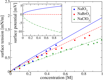
Figure 4: Surface tensions for NaIO3, NaBrO3 and NaClO3. The symbols are experimental data ³³ and the lines are obtained using the present theory. The inset shows the electrostatic surface potential difference and has the same horizontal axis label as the main figure.

However, since the polarizability is, in general, proportional to the volume of an ion, we can easily estimate it based on the polarizability of iodate, which is given in the reference ³⁰, $\gamma_{IO_{3}}=8.0$ ų. We then obtain $\gamma_{ClO_{3}}=5.3$ ų. Using eq 2, we can now calculate the surface potential, the ionic density distribution and, integrating the Gibbs adsorption isotherm, the excess surface tension, 4, 5, 6, 7, and 8. We stress that in all the calculations we are using the same value of sodium hydrated radius, $a_{h}=2.5$ Å, obtained for halogen salts. For nitrate and chlorate, the predictions of the theory are in good agreement with the experimental measurements of Matubayasi ³³, see 4 and 5.

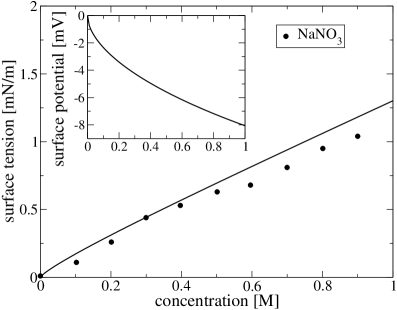
Figure 5: Surface tension of NaNO3. The symbols are the experimental data ³³ and the lines are the present theory. The inset shows the electrostatic surface potential difference vs. the molar concentration.

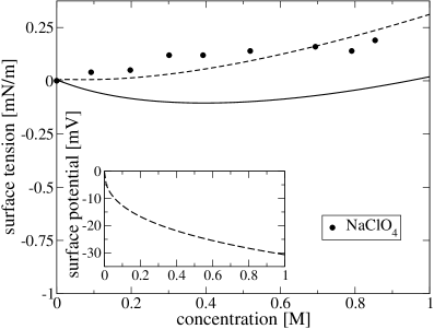
Figure 6: Surface tensions of NaClO4. The symbols are the experimental data ³³ and the lines are the present theory. The solid line is obtained using $a_{ClO_{4}}=2.83$ Å from eq. (16), and the dashed line using $a_{ClO_{4}}=2.75$ Å. The inset shows the electrostatic surface potential difference vs. the molar concentration.

For perchlorate, the theoretical surface tension is slightly lower than what was found experimentally, 6. The difficulty is that since the cavitational energy scales with the volume of the ion, for large ions it becomes very sensitive to the precise value of the ionic radius. For example, if we use a slightly smaller radius of perchlorate $a_{ClO_{4}}=2.75$ Å, we obtain a good agreement with experiment, 6. The theory shows that ClO4- is adsorbed stronger than either ClO3- or I-, see 7 and 8. This is conclusion is also in agreement with the simulations ⁴⁰.

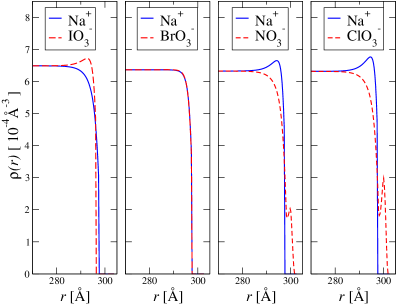
Figure 7: Theoretical ionic density profiles for NaIO3, NaBrO3, NaNO3 and NaClO3 at $1$M. The GDS is at $r=300$ Å.

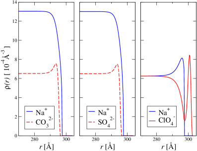
Figure 8: Theoretical ionic density profiles for Na2CO3, Na2SO4 and NaClO4 at $1$M. The GDS is at $r=300$ Å.

We next calculate the surface tension of sodium salts with kosmotropic anions. Since the $B$-coefficient of iodate is so large, we expect that this ion will remain completely hydrated near the GDS. The bulk hydrated radius of IO3- is $a_{h}=3.74$ ų⁴. Using this in eq 14, we obtain an excellent agreement with the experimental data ³³, 4. The $B$-coefficient of bromate is almost zero, so that BrO3- should be only very weakly hydrated near the GDS. Indeed, using $a_{h}=2.41$ Å, we obtain a very good agreement with the experimental data ³³, 4. This value is only slightly above the crystallographic radius of BrO3-, $a_{BrO_{3}}=2.31$ Å, obtained using eq 16.

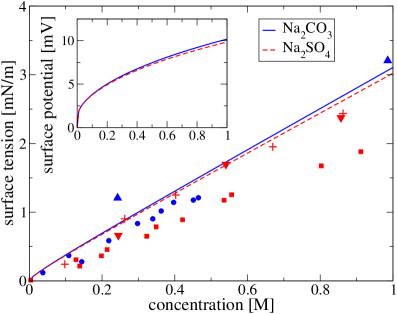
Figure 9: Surface tensions of Na2CO3 and Na2SO4. The circles and the squares are the experimental data for sodium carbonate and soldium sulfate, respectively ³¹ . The up and down triangles are the data of Jarvis and Scheiman ³⁷. The plus symbols are the data of Weissenborn and Pugh ⁴¹ for the Na2SO4 salt. The lines are the present theory. The inset shows the surface potential difference vs. the molar concentration.

Finally, we consider the surface tension of sodium salts with divalent anion. The predictions of the theory, in this case, should be taken with a grain of salt, since it is well known that Poisson-Boltzmann theory begins to loose its validity for divalent ion as a result of inter-ionic correlations ⁴². Nevertheless, it is curious to see how well the theory does in this limiting case. The $B$-coefficients of SO4^2- and CO3^2- are large and positive, so that we expect these ions to be fully hydrated, $a_{h}=3.79$ Å and $3.94$ Å ³⁴, respectively. Calculating the surface tensions, we find that our results are somewhat above those measured by Matubayasi et al. ³¹ . Curiously, the theory agrees well the measurements of Jarvis and Scheiman ³⁷ and of Weissenborn and Pugh ⁴¹, 9. At this point we do not know what to make of this agreement. The surface potentials of sodium sulfate and sodium carbonate are listed in 1. In 3 we summarize the classification of all ions and the radii used in calculations.

Table 3: Ion classification into chaotropes (c) and kosmotropes (k) and their effective radii. The kosmotropic radii listed are either hydrated or partially hydrated. The chaotropic radii are the bare ones, for oxy-anions given by eq 16.

Ions	chao/kosmo	radius (Å)
Na+	k	2.5
F-	k	3.54
Cl-	k	2
Br-	c	2.05
I-	c	2.26
IO3-	k	3.74
BrO3-	k	2.41
NO3-	c	1.98
ClO3-	c	2.16
ClO4-	c	2.83
CO3^2-	k	3.94
SO4^2-	k	3.79

5 Conclusions

We have presented a theory which allows us to quantitatively calculate the surface tensions and the surface potentials of 10 sodium salts with only one adjustable parameter, the partial hydrated radius of the sodium cation. We find that anions near the GDS can be classified into kosmotropes and chaotropes. Kosmotropes remain hydrated near the interface, while the chaotropes loose their hydration sheath. For all salts studied in this paper, the classification of ions into the structure makers/breakers agrees with the bulk characterization based on the Jones-Dole viscosity $B$-coefficient. If anions are arranged in the order of increasing electrostatic surface potential difference, we obtain the extended lyotropic (Hofmeister) series, CO3^2- > SO4^2- > IO3- > F- > BrO3- > Cl- > NO3- > Br- > ClO3- > I- > ClO4-. To our knowledge this is the first time that this sequence has been derived theoretically. The theory also helps to understand why Hofmeister series is relevant to biology ^{43, *ZhCr06}. In general, proteins have both hydrophobic and hydrophilic moieties. If the hydrophobic region is sufficiently large, it can become completely dewetted ^{26, *Ch05}, surrounded by a vapor-like film into which chaotropic anions can become adsorbed. This will help to solvate proteins, but at the same time will destroy their tertiary structure, denaturing them in the process. On the other hand, the kosmotropic ions will favor protein precipitation. The action is again two fold. The kosmotropes adsorb water which could, otherwise, be used to solvate hydrophilic moieties. They also screen the electrostatic repulsion, allowing charged proteins to come into a close contact and to stick together as the result of their van der Waals and hydrophobic interactions. This leads to formation of large clusters which can no longer be dispersed in water and must precipitate.

We thank Prof. Norihiro Matubayasi for providing us with the unpublished data for the surface tensions of chlorate, bromate, iodate and perchlorate. YL is also grateful to Dr. Delfi Bastos González for first bringing the kosmotropic nature of iodate to his attention.

References

- Heydweiller 1910 Heydweiller, A. Ann. Phys. (Leipzig) 1910, 33, 145
- Langmuir 1917 Langmuir, I. J. Am. Chem. Soc. 1917, 39, 1848
- Harkins and McLaughlin 1925 Harkins, W. D.; McLaughlin, H. M. ibid. 1925, 47, 2083
- Harkins and Gilbert 1926 Harkins, W. D.; Gilbert, E. C. ibid. 1926, 48, 604
- Wagner 1924 Wagner, C. Phys. Z. 1924, 25, 474
- Debye and Hückel 1923 Debye, P. W.; Hückel, E. Phys. Z. 1923, 24, 185
- Onsager and Samaras 1934 Onsager, L.; Samaras, N. N. T. J. Chem. Phys. 1934, 2, 528
- Long and Nutting 1942 Long, F. A.; Nutting, G. C. J. Am. Chem. Soc. 1942, 64, 2476
- Passoth 1959 Passoth, G. Z. Phys. Chem. (Leipzig) 1959, 211, 129
- Levin and Flores-Mena 2001 Levin, Y.; Flores-Mena, J. E. Europhys. Lett. 2001, 56, 187
- Frumkin 1924 Frumkin, A. Z. Phys. Chem. 1924, 109, 34
- Boström et al. 2001 Boström, M.; Williams, D. R. M.; Ninham, B. W. Langmuir 2001, 17, 4475
- Perera and Berkowitz 1991 Perera, L.; Berkowitz, M. L. J. Chem. Phys. 1991, 95, 1954
- Dang and Smith 1993 Dang, L. X.; Smith, D. E. J. Chem. Phys. 1993, 99, 6950
- Stuart and Berne 1999 Stuart, S. J.; Berne, B. J. J. Phys. Chem. A 1999, 103, 10300
- Jungwirth and Tobias 2002 Jungwirth, P.; Tobias, D. J. J. Phys. Chem. B 2002, 106, 6361
- Jungwirth and Tobias 2006 Jungwirth, P.; Tobias, D. J. Chem. Rev. 2006, 106, 1259
- Horinek and Netz 2007 Horinek, D.; Netz, R. R. Phys. Rev. Lett. 2007, 99, 226104
- Brown et al. 2008 Brown, M. A.; D’Auria, R.; Kuo, I. F. W.; Krisch, M. J.; Starr, D. E.; Bluhm, H.; Tobias, D. J.; JC, J. C. H. Phys. Chem. Chem. Phys. 2008, 10, 4778
- Markovich et al. 1991 Markovich, G.; Pollack, S.; Giniger, R.; Cheshnovski, O. J. Chem. Phys. 1991, 95, 9416
- Ghosal et al. 2005 Ghosal, S.; Hemminger, J.; Bluhm, H.; Mun, B.; Hebenstreit, E. L. D.; Ketteler, G.; Ogletree, D. F.; Requejo, F. G.; Salmeron, M. Science 2005, 307, 563
- Garrett 2004 Garrett, B. Science 2004, 303, 1146
- Levin 2009 Levin, Y. Phys. Rev. Lett. 2009, 102, 147803
- Levin et al. 2009 Levin, Y.; dos Santos, A. P.; Diehl, A. Phys. Rev. Lett. 2009, 103, 257802
- Ho et al. 2003 Ho, C. H.; Tsao, H. K.; Sheng, Y. J. J. Chem. Phys. 2003, 119, 2369
- Lum et al. 1999 Lum, K.; Chandler, D.; Weeks, J. D. J. Phys. Chem. B 1999, 103, 4570
- Chandler 2005 Chandler, D. Nature (London) 2005, 437, 640
- Rajamani et al. 2005 Rajamani, S.; Truskett, T. M.; Garde, S. Proc. Natl. Acad. Sci. U.S.A. 2005, 102, 9475
- Latimer et al. 1939 Latimer, W. M.; Pitzer, K. S.; Slansky, C. M. J. Chem. Phys. 1939, 7, 108
- Pyper et al. 1992 Pyper, N. C.; Pike, C. G.; Edwards, P. P. Mol. Phys. 1992, 76, 353
- Matubayasi et al. 2001 Matubayasi, N.; Tsunemoto, K.; Sato, I.; Akizuki, R.; Morishita, T.; Matuzawa, A.; Natsukari, Y. J. Colloid Interface Sci. 2001, 243, 444
- Matubayasi et al. 1999 Matubayasi, N.; Matsuo, H.; Yamamoto, K.; Yamaguchi, S.; Matuzawa, A. J. Colloid Interface Sci. 1999, 209, 398
- 33 Matubayasi, N. (unpublished)
- Nightingale Jr. 1959 Nightingale Jr., E. R. J. Phys. Chem. 1959, 63, 1381
- Raymond and Richmond 2004 Raymond, E. A.; Richmond, G. L. J. Phys. Chem. B 2004, 108, 5051
- Randles, J. E. B. 1963 Randles, J. E. B., Advances in Electrochemistry and Electrochemical Engineering; Interscience: New York, 1963; Vol. 3, p 1
- Jarvis and Scheiman 1968 Jarvis, N. L.; Scheiman, M. A. J. Phys. Chem. 1968, 72, 74
- Jenkins and Marcus 1995 Jenkins, H. D. B.; Marcus, Y. Chem. Rev. 1995, 95, 2695
- Couture and Laidler 1957 Couture, A. M.; Laidler, K. L. Can. J. Chem. 1957, 35, 202
- Ottosson et al. 2009 Ottosson, N.; Vacha, R.; Aziz, E. F.; Pokapanich, W.; Eberhardt, W.; Svensson, S.; Ohrwall, G.; Jungwirth, P.; Bjorneholm, O.; B, B. W. J. Chem. Phys. 2009, 131, 124706
- Weissenborn and Pugh 1996 Weissenborn, P. K.; Pugh, R. J. J. Colloid Interface Sci. 1996, 184, 550
- Levin 2002 Levin, Y. Rep. Prog. Phys. 2002, 65, 1577
- Collins and Washanbaugh 1985 Collins, K. D.; Washanbaugh, M. W. Quaterly Rev. Biophys. 1985, 18, 323
- Zhang and Cremer 2006 Zhang, Y.; Cremer, P. S. Curr. Opin. Chem. Biol. 2006, 10, 658