Calculation of transition probabilities and ac Stark shifts in two-photon laser transitions of antiprotonic helium

Abstract

Numerical ab initio variational calculations of the transition probabilities and ac Stark shifts in two-photon transitions of antiprotonic helium atoms driven by two counter-propagating laser beams are presented. We found that sub-Doppler spectroscopy is in principle possible by exciting transitions of the type $(n,L)$$\rightarrow$$(n-2,L-2)$ between antiprotonic states of principal and angular momentum quantum numbers $n\sim L-1\sim 35$, first by using highly monochromatic, nanosecond laser beams of intensities $10^{4}-10^{5}$ W/cm², and then by tuning the virtual intermediate state close (e.g., within 10–20 GHz) to the real state $(n-1,L-1)$ to enhance the nonlinear transition probability. We expect that ac Stark shifts of a few MHz or more will become an important source of systematic error at fractional precisions of better than a few parts in $10^{9}$. These shifts can in principle be minimized and even canceled by selecting an optimum combination of laser intensities and frequencies. We simulated the resonance profiles of some two-photon transitions in the regions $n=30$–40 of the $\overline{p}{\rm{}^{4}He}^{+}$ and $\overline{p}{\rm{}^{3}He}^{+}$ isotopes to find the best conditions that would allow this.

I Introduction

The transition frequencies $\nu_{\rm exp}$ of antiprotonic helium atoms Hayanorpp ; PhysRep ; Mor94 ; Maas ; Tor99 ($\overline{p}{\rm He}^{+}\equiv\overline{p}^{-}+e^{-}+{\rm He}^{2+}$) have recently been measured by single-photon laser spectroscopy to a fractional precision of $\sim 1$ part in $10^{8}$ Hori01 ; Hori03 ; Hori06 . By comparing these results with three-body QED calculations Kor00 ; Kor03 ; Kor08 ; kino2004 ; andersson , the antiproton-to-electron mass ratio has been determined as 1836.152674(5) Hori06 ; CODATA06 . To further increase the experimental precision on $\nu_{\rm exp}$, we have proposed future experiments hori2000 of sub-Doppler two-photon spectroscopy of $\overline{p}{\rm He}^{+}$ by irradiating the atom with two counter-propagating laser beams horiopt09 . Dynamic (ac) Stark effects are expected to become one of the important sources of systematic error in these future experiments, as is the case with other high-precision laser spectroscopy measurements of atomic hydrogen Hansch86 ; garreau ; fischer ; Haas2006 ; Haas2006_2 ; kolachevsky and antihydrogen gabrielse ; andresen , molecular hydrogen hannemann ; hilico , helium eikema1996 ; eikema1997 ; minardi ; bergeson , and muonium yakhontov96 ; yakhontov99 ; meyer . In this paper we calculate the transition probability and ac Stark shift involved in these two-photon transitions using precise three-body wavefunctions of $\overline{p}{\rm He}^{+}$.

The $\overline{p}{\rm He^{+}}$ atoms PhysRep can be easily synthesized by simply allowing an antiproton beam to slow down knudsen ; foster ; luhr2009 ; henkel2009 ; mcgovern ; barna and come to rest in a helium target. Some of the antiprotons are captured mhori2002 ; mhori2004 ; briggs1999 ; cohen2004 ; hesse ; tokesi ; ovchinnikov ; revai06 ; tong08 ; genkin into Rydberg $\overline{p}{\rm He}^{+}$ states with large principal ($n\sim 38$) and angular momentum ($L\sim n-1$) quantum numbers that have microsecond-scale lifetimes against antiproton annihilation in the helium nucleus. The longevity is due to the ground-state electron in $\overline{p}{\rm He}^{+}$ which protects the antiproton during collisions with other helium atoms mhori1997 ; russell02 ; obreshkov . All laser spectroscopy experiments Hori06 reported so far have used pulsed lasers ol2003 to induce single-photon transitions of antiprotons occupying these metastable states, to short-lived states with nanosecond-scale lifetimes against Auger emission of the electron yamaguchi2002 ; yamaguchi2004 ; kor97 ; revai97 ; kartavtsev2000 . A Rydberg $\overline{p}{\rm He}^{2+}$ ion mhori2005 ; sakimoto2007 ; korenman07 ; sakimoto2009 then remained after Auger decay, which was rapidly destroyed by collisional Stark effects. The resulting resonance profiles of $\overline{p}{\rm He}^{+}$ had Doppler widths $\Delta\omega_{D}/2\pi\sim 0.3-1.2$ GHz corresponding to the thermal motion of $\overline{p}{\rm He}^{+}$ in the experimental target at $T=10$ K. This broadening limited the experimental precision on $\nu_{\rm exp}$.

The first-order Doppler broadening can in principle be reduced (Fig. 1) hori2000 by irradiating $\overline{p}\mbox{He}^{+}$ atoms with two counter-propagating laser beams of angular frequencies $\omega_{1}$ and $\omega_{2}$ and inducing, e.g., the two-photon transition $(n,L)\!\to\!(n\!-\!2,L\!-\!2)$. This results in a reduction of $\Delta\omega_{D}$ by a factor $|(\omega_{1}-\omega_{2})/(\omega_{1}+\omega_{2})|$. Among a number of possible two-photon transitions, a particularly strong signal is expected for $(n,L)\!=\!(36,34)\!\to\!(34,32)$ (Fig. 1), as this involves a large antiproton population mhori2002 ; mhori2004 in the resonance parent state $(36,34)$. Whereas the states $(36,34)$ and $(35,33)$ are metastable with 1-$\mu{\rm s}$-scale lifetimes, the resonance daughter state $(34,32)$ is Auger-dominated with the lifetime $\tau\sim 4$ ns Hori01 ; Kor03 ; yamaguchi2002 ; yamaguchi2004 that corresponds to the natural width of a spectral line of $\sim\!30$ MHz.

The probability of inducing the transition can be enhanced hori2000 ; bjorkholm ; salomaa1975 ; salomaa1976 ; salomaa1977 ; bordo ; fort95 ; wei98 by tuning $\omega_{1}$ and $\omega_{2}$ so that the virtual intermediate state of the two-photon transition lies close (e.g. $|\Delta\omega_{d}/2\pi|<$ 10–20 GHz) to the real state $(35,33)$ such that,

$$\begin{array}[]{@{}l}\displaystyle\omega_{1}{(\rm SI)}=4\pi R_{\infty}c\left[E_{(35,33)}-E_{(34,32)}{(\rm a.u.)}\right]+\Delta\omega_{d},\\[11.38109pt] \displaystyle\omega_{2}{(\rm SI)}=4\pi R_{\infty}c\left[E_{(36,34)}-E_{(35,33)}{(\rm a.u.)}\right]-\Delta\omega_{d}.\end{array}$$ (1)

Here $R_{\infty}c=3.289842\!\times\!10^{15}$ Hz denotes the Rydberg constant, and $E_{(n,L)}$ the binding energy of the $\overline{p}{\rm{}^{4}He}^{+}$ state $(n,L)$ in atomic units. At experimental conditions wherein this offset is much larger than the Doppler width ($|\Delta\omega_{d}|\gg\Delta\omega_{D}$), the two-photon transition is expected to directly transfer the antiprotons populating the parent state $(36,34)$ to the daughter state $(34,32)$, whereas the population in the intermediate state $(35,33)$ will be unaffected.

This paper is organized in the following way. Some details of the numerical methods are described in Section II. The transition amplitude of the two-photon resonance $(36,34)$$\rightarrow$$(34,32)$ of $\overline{p}{\rm{}^{4}He}$, and the polarizabilities of the parent and daughter states $(36,34)$ and $(34,32)$ at various offsets $\Delta\omega_{d}$ are estimated in Sections III.1 and III.2. We next calculate the ”background” polarizability due to the contributions of $\overline{p}{\rm He}^{+}$ states other than the resonant intermediate state $(35,33)$ (Section III.3). Based on these results, the ac Stark shift and broadening are semi-analytically estimated in Section III.4. We next discuss the hyperfine structure in two-photon transitions of the $\overline{p}{\rm{}^{4}He}^{+}$ and $\overline{p}{\rm{}^{3}He}^{+}$ isotopes (Section III.5) pask09 ; bakahfs ; yam01 ; kinohfs ; Kor06 ; bakalov07 . We numerically simulate the profile of several two-photon resonances (Section III.6) before concluding the paper. Atomic units are used to evaluate the state polarizabilities and transition amplitudes khadjavi ; chung1992 ; bonin ; bhatia ; michel ; masili , whereas International System of Units (SI) are used for the transition frequencies, rates, and laser intensities relevant for future spectroscopy experiments.

II Details of the calculation

For simplicity we take the linearly polarized laser field aligned along the $z$-axis, such that the perturbation Hamiltonian in a laser field of frequency $\omega$ and amplitude $F$ has the form,

$$H^{\prime}=-e\,\mathbf{F}(t)\,\mathbf{d},\qquad\mathbf{F}(t)=\mathbf{e}_{z}F\cos(wt).$$ (2)

Here $\mathbf{d}=\sum_{a=1}^{3}Z_{a}\mathbf{R}_{a}$ is the electric dipole moment operator. The second order correction $E^{(2)}$ to the unperturbed eigenenergy $E_{0}$ of a $\overline{p}{\rm He}^{+}$ state vector $|0\rangle$ may then be expressed as,

$$E^{(2)}=-\,\frac{1}{2}\>\alpha_{d}^{zz}(\omega,M^{2})\cdot F^{2},$$ (3)

where $a_{d}^{ij}(\omega)$ is a tensor of the dynamic dipole polarizability:

$$\alpha_{d}^{ij}=-\sum_{q}\left[\frac{\langle 0|d^{i}|q\rangle\langle q|d^{j}|0\rangle}{E_{0}-E_{q}+\omega}+\frac{\langle 0|d^{i}|q\rangle\langle q|d^{j}|0\rangle}{E_{0}-E_{q}-\omega}\right].$$ (4)

The energy of a $\overline{p}{\rm He}^{+}$ state vector $|q\rangle$ is denoted by $E_{q}$, and the summation of $q$ is over all states which are accessible via single-photon transition from the resonance parent state $|0\rangle$.

The tensor $a_{d}^{ij}(\omega)$ may be rewritten in terms of the irreducible scalar and tensor polarizability operators,

$$\begin{array}[]{@{}l}\displaystyle\alpha_{d}^{ij}=\alpha_{s}+\alpha_{t}\left[\hat{L}^{i}\hat{L}^{j}+\hat{L}^{j}\hat{L}^{i}-\frac{2}{3}\mathbf{\hat{L}}^{2}\right],\\[8.53581pt] \displaystyle\alpha_{s}=\frac{1}{3}\bigl{[}a_{+}+a_{0}+a_{-}\bigr{]},\\[8.53581pt] \displaystyle\alpha_{t}=-\frac{a_{+}L(2L\!-\!1)}{3(L\!+\!1)(2L\!+\!3)}+\frac{a_{0}(2L\!-\!1)}{3(L\!+\!1)}-\frac{a_{-}}{3}\>,\end{array}$$ (5)

where the angular momentum operator is denoted by $\hat{L}$. The coefficients $a_{+}$, $a_{0}$, and $a_{-}$ are defined as follows,

$$\begin{array}[]{@{}l}\displaystyle a_{+}=-\frac{2}{2L+1}\sum_{q}\frac{(E_{0}\!-\!E_{q})\bigl{|}\langle 0L\|\mathbf{d}\|q(L\!+\!1)\rangle\bigr{|}^{2}}{(E_{0}-E_{q})^{2}-\omega^{2}},\\[11.38109pt] \displaystyle a_{0}=-\frac{2}{2L+1}\sum_{q}\frac{(E_{0}\!-\!E_{q})\bigl{|}\langle 0L\|\mathbf{d}\|qL\rangle\bigr{|}^{2}}{(E_{0}-E_{q})^{2}-\omega^{2}},\\[11.38109pt] \displaystyle a_{-}=-\frac{2}{2L+1}\sum_{q}\frac{(E_{0}\!-\!E_{q})\bigl{|}\langle 0L\|\mathbf{d}\|q(L\!-\!1)\rangle\bigr{|}^{2}}{(E_{0}-E_{q})^{2}-\omega^{2}}.\end{array}$$ (6)

Here $a_{+}$ and $a_{-}$ represent the contributions from antiproton transitions to states of normal parity which change the orbital angular momentum quantum number $L$ of the antiproton by 1 or $-1$. The contribution $a_{0}$ involves transitions to $\overline{p}{\rm He}^{+}$ states of anomalous parity wherein the $L$-value is unchanged and the 1s-electron is excited to, e.g., the $2p$ state.

For our analysis it is convenient to define ”background” polarizabilities using the above equations, wherein the dominant contribution from the intermediate state of the two-photon transition is subtracted. For example, the corresponding scalar and tensor background polarizabilities of state $(n,L)=(36,34)$ can be calculated as,

$$\begin{array}[]{@{}l}\displaystyle\beta_{s}=\alpha_{s}+\frac{2\left(E_{0}\!-\!E_{i}\right)}{3(2L\!+\!1)}\cdot\frac{~{}\bigl{|}\langle 0L\|\mathbf{d}\|i(L\!-\!1)\rangle\bigr{|}^{2}}{\left(E_{0}-E_{i}\right)^{2}-\omega^{2}},\\[8.53581pt] \displaystyle\beta_{t}=\alpha_{t}-\frac{2(E_{0}\!-\!E_{i})}{3(2L\!+\!1)}\cdot\frac{~{}\bigl{|}\langle 0L\|\mathbf{d}\|i(L-1)\rangle\bigr{|}^{2}}{(E_{0}-E_{i})^{2}-\omega^{2}}.\end{array}$$ (7)

Here $E_{0}$ and $E_{i}$ denote the energies of state $(36,34)$ and the intermediate state $(35,32)$.

The transition matrix element $\kappa_{L,L-2,M}$ of the $\overline{p}{\rm He}^{+}$ two-photon transition $(n,L,M)$$\rightarrow$$(n\!-\!2,L\!-\!2,M)$ induced by two linearly-polarized laser beams can be calculated using the Wigner $3j$-symbols as,

$$\begin{array}[]{@{}l}\displaystyle\kappa_{L,L\!-2,M}=-\!\left(\begin{array}[]{@{\,}c@{\;}c@{\;}c@{\,}}L\!-\!1&1&L\\ M&0&-M\end{array}\right)\left(\begin{array}[]{@{\,}c@{\;\,}c@{\;\,}c@{\,}}L\!-\!1&1&L\!-\!2\\ M&0&-M\end{array}\right)\!\!\!\\[14.22636pt] \displaystyle\hskip 14.22636pt\times\sum_{q}\biggl{[}\frac{\langle 1(L\!-\!2)\|\mathbf{d}\|q(L\!-\!1)\rangle\langle q(L\!-\!1)\|\mathbf{d}\|0L\rangle}{E_{0}-E_{q}-\omega_{1}}\\[11.38109pt] \displaystyle\hskip 39.83385pt+\frac{\langle 1(L\!-\!2)\|\mathbf{d}\|q(L\!-\!1)\rangle\langle q(L\!-\!1)\|\mathbf{d}\|0L\rangle}{E_{0}-E_{q}-\omega_{2}}\biggr{]},\end{array}$$ (8)

wherein $|1\rangle$ denotes the state vector of the resonance daughter state. This is related to the two-photon Rabi oscillation frequency (in atomic units) of this laser transition via the equation,

$$\frac{\Omega_{2\gamma M}}{2\pi}=\frac{1}{2}\left|\kappa_{L,L-2,M}\right|F_{1}F_{2}.$$ (9)

The last term in Eq. (8) gives a small contribution and will be neglected.

In order to calculate these quantities we must evaluate the reduced matrix elements for the dipole operator $\mathbf{d}$ and diagonalize the Hamiltonian. For this we use the variational exponential expansion described in Ref. Kor00 . The wave function for a state with a total orbital angular momentum $L$ and of a total spatial parity $\pi=(-1)^{L}$ is expanded as follows,

$$\begin{array}[]{@{}l}\displaystyle\Psi_{LM}^{\pi}(\mathbf{R},\mathbf{r}_{1})=\sum_{l_{1}+l_{2}=L}\mathcal{Y}^{l_{1}l_{2}}_{LM}(\hat{\mathbf{R}},\hat{\mathbf{r}}_{1})G^{L\pi}_{l_{1}l_{2}}(R,r_{1},r_{2}),\\[11.38109pt] \displaystyle G_{l_{1}l_{2}}^{L\pi}(R,r_{1},r_{2})=\sum_{n=1}^{N}\Big{\{}C_{n}\,\mbox{Re}\bigl{[}e^{-\alpha_{n}R-\beta_{n}r_{1}-\gamma_{n}r_{2}}\bigr{]}\\[5.69054pt] \displaystyle\hskip 85.35826pt+D_{n}\,\mbox{Im}\bigl{[}e^{-\alpha_{n}R-\beta_{n}r_{1}-\gamma_{n}r_{2}}\bigr{]}\Big{\}}.\end{array}$$ (10)

where the complex exponents $\alpha$, $\beta$, and $\gamma$ are generated in a pseudorandom way, $\mathbf{R}$ and $\mathbf{r}_{1}$ are position vectors of an antiproton and an electron with respect to a helium nucleus, and $r_{2}$ the distance between the antiproton and electron. Further details may be found in Refs. Kor00 ; Kor03 .

III Results

III.1 Transition matrix element

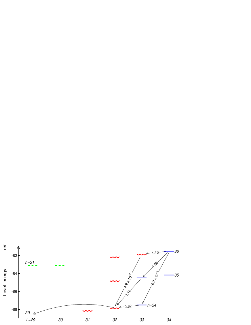
Figure 2: Portion of the energy level diagram of $\overline{p}{\rm{}^{4}He}^{+}$. The solid lines indicate radiation-dominated metastable states, the wavy lines Auger-dominated short-lived states. The broken lines indicate $\overline{p}{\rm He}^{2+}$ ionic states formed after Auger emission, the curved arrows indicate Auger transitions with minimum $|\Delta L|$. Calculated values of the dipole moments for some single-photon radiative transitions are shown in atomic units.

We first calculated the transition amplitude $\kappa_{L,L-2,M}$ for the two-photon resonance $(n,L)=(36,34)$$\rightarrow$$(34,32)$ in $\overline{p}{\rm{}^{4}He}^{+}$ at various offsets $\omega_{d}$ from the intermediate $(35,33)$ state, and estimated the laser intensities needed to drive this transition. In Fig. 2, sequences of single-photon transitions connecting the states $(36,34)$ and $(34,32)$ are indicated by straight arrows, together with the corresponding dipole moment $|\langle 0L\|\mathbf{d}\|q(L-1)\rangle|$. The atomic units shown here can be converted to SI units, the corresponding spontaneous decay rates in s^-1 may be obtained using the equation,

$$\gamma{\rm(SI)}=\frac{e^{2}a_{0}^{2}}{4\pi\epsilon_{0}}\frac{4\omega^{3}_{q0}}{3\hbar c^{3}}\frac{|\langle 0L\|\mathbf{d}\|q(L-1)\rangle|^{2}{\rm(a.u.)}}{2L+1}.$$ (11)

The SI-unit constants that appear in the above equation are, $e$: the elementary charge, $a_{0}$: the Bohr radius, $\epsilon_{0}$: the dielectric constant of vacuum, $\hbar$: the reduced Planck constant, and $c$ the speed of light. The angular transition frequency between states $|q\rangle$ and $|0\rangle$ are denoted by $\omega_{q0}$.

Two types of transitions $(n,L)\rightarrow(n,L\!-\!1)$ and $(n,L)$$\rightarrow$$(n\!-\!1,L\!-\!1)$ have the largest amplitudes of $\sim 1$ a.u., but the later kind which conserve the vibrational quantum number $v=n\!-\!L\!-\!1$ and involve fluorescence photons of frequency $\omega_{q0}/2\pi\sim 10^{15}$ Hz constitute the dominant channels of spontaneous decay. These transitions are most favorable for laser spectroscopy. The transition frequencies, dipole moments, and decay rates of some single-photon resonances in $\overline{p}{\rm{}^{4}He}^{+}$ and $\overline{p}{\rm{}^{3}He}^{+}$ of the type $(n,L)$$\rightarrow$$(n\!-\!1,L\!-\!1)$ are shown in Table 1. The dipole moments for the higher-lying infrared transitions involving states with $n\sim 40$ are relatively large ($>2$ a.u.), whereas for UV transitions in the $n\leq 33$ regions it is reduced to $<1$ a.u. On the other hand, the radiative decay rates increase for lower-$n$ transitions, e.g. from $4.7\times 10^{5}$ s^-1 for $(40,36)$$\rightarrow$$(39,35)$, to $6.6\times 10^{5}$ s^-1 for $(32,31)$$\rightarrow$$(31,30)$ due to the $\omega^{3}$-dependence.

Using the single-photon dipole moments calculated above, we derive the two-photon transition amplitude $\kappa_{L,L-2,M}$ of the resonance $(36,34)$$\rightarrow$$(34,32)$ in $\overline{p}{\rm{}^{4}He}^{+}$ for cases wherein the virtual intermediate state is offset over a large range between $\Delta\omega_{d}/2\pi=-0.7$ and 0.7 PHz from the state $(35,33)$. The atom is excited by two linearly-polarized, counterpropagating laser beams. Fig. 3 (a)–(c) show the amplitude $\kappa_{L,L-2}$ averaged over all $\sim 70$ transitions between the magnetic substates which conserve the $M$-value. The $|\kappa_{L,L-2}|$-values are usually small, e.g. $\sim 1$ a.u. for lasers of equal frequency ($\omega_{1}=\omega_{2}$). This is an order of magnitude smaller than the amplitude $\sim 7.8$ a.u. Haas2006 for the 1s-2s two-photon transition of atomic hydrogen excited by 243-nm laser light. Gigawatt-scale laser intensities would be needed to induce the antiprotonic transition within the microsecond-scale lifetime of $\overline{p}{\rm He}^{+}$. On the other hand, the transition probabilities can be strongly enhanced to $>10^{3}$ a.u. by tuning the virtual intermediate state within $\sim 20$ GHz of the real states $(n,L)=(34,33)$, $(35,33)$, or $(36,33)$. Eq. 9 indicates that the transition can then be induced using nanosecond laser pulses of electric field $F\sim(1-2)\times 10^{-6}$ a.u. According to the equation,

$$I({\rm SI})=\frac{1}{2}\epsilon_{0}c\left(\frac{eF(\rm a.u.)}{4\pi\epsilon_{0}a_{0}^{2}}\right)^{2},$$ (12)

this corresponds to a peak intensity of $I\sim 10^{4}$–$10^{5}$ W/cm² which is achievable using titanium sapphire lasers of narrow linewidth horiopt09 .

III.2 Polarizabilities

We next evaluate the polarizabilities of the parent and daughter states of the transition. In Figs. 4 (a) and (c), the scalar and tensor polarizability components, $\alpha_{s}(\omega_{1})_{(34,32)}$, $\alpha_{t}(\omega_{1})_{(34,32)}$, of state $(n,L)=(34,32)$ are shown. To simplify the calculation, we initially assume that the atom is irradiated by a single laser field of frequency $\omega_{1}$ (see Fig. 1) corresponding to offsets between $\Delta\omega_{d}/2\pi=-20$ and 20 GHz from the state $(35,33)$. A similar plot for the polarizabilities $\alpha_{s}(\omega_{2})_{(36,34)}$ and $\alpha_{t}(\omega_{2})_{(36,34)}$ of state $(36,34)$ irradiated by a laser field of $\omega_{2}$ are shown in Figs. 4 (b) and (d).

As the respective lasers are offset from $\Delta\omega_{d}/2\pi=-100$ to -6 GHz, the scalar polarizabilities decrease from $\sim-500$ to $\sim-1\times 10^{4}$ a.u., whereas the tensor polarizabilities have opposite sign and increase from $\sim 500$ to $\sim 1\times 10^{4}$ a.u. (Table  2). Polarizabilities of 1000–10000 a.u. correspond to 50–500 Hz/(W/cm²) in SI units according to the equation,

$$\alpha({\rm a.u.})=\alpha({\rm SI})\times\frac{\hbar^{2}}{m_{e}a_{0}^{4}\alpha}.$$ (13)

These graphs follow a reciprocal $\Delta\omega_{d}^{-1}$ dependence and are approximately symmetric with respect to the origin. This simple behavior suggests that the ac Stark shift is primarily caused by the contribution from the intermediate state $(35,33)$.

III.3 Contribution of nonresonant states

We next study the non-resonant or ”background” contributions (Eq. 7) to the polarizabilities from all $\overline{p}{\rm He}^{+}$ states other than the intermediate state $(n,L)=(35,33)$. This will allow us to estimate how far the measured ac-Stark shift would deviate from the predictions of a simple three-level model which include only the resonance parent, daughter, and intermediate states. Figs. 5 (a) and (c) show the background scalar and tensor polarizabilities $\beta_{s}(\omega_{2})_{(36,34)}$ and $\beta_{t}(\omega_{2})_{(36,34)}$ of state $(36,34)$ when irradiated with a single laser field of frequency $\omega_{2}$ at offsets between $\Delta\omega_{d}/2\pi=-20$ and 20 GHz. They remained relatively constant at $\sim\!-0.40$ and $0.95$ a.u. respectively (Table 2). Figs. 5 (b) and (d) are the corresponding plots of $\beta_{s}(\omega_{1})_{(34,32)}$ and $\beta_{t}(\omega_{1})_{(34,32)}$ for state $(34,32)$ irradiated with the $\omega_{1}$-laser. They are similarly constant ($-1.36$ and $-0.40$ a.u.). All these background polarizabilities are at least three orders of magnitude smaller than the dominant contributions to $\alpha_{s}$ and $\alpha_{t}$ arising from the intermediate state $(35,33)$ at offsets $|\Delta\omega_{d}/2\pi|<12$ GHz.

The case of two counterpropagating laser fields of angular frequencies $\omega_{1}$ and $\omega_{2}$, and amplitudes $F_{1}$ and $F_{2}$ irradiating the atom simultaneously will next be considered. The perturbation Hamiltonian for this can be expressed as,

$$\begin{array}[]{@{}l}H^{\prime}=-e\,\mathbf{F}(t)\,\mathbf{d},\\[5.69054pt] \mathbf{F}(t)=\mathbf{e}_{z}\left[F_{1}\cos(w_{1}t)\!+\!F_{2}\cos(w_{2}t)\right].\end{array}$$ (14)

As shown in Ref. Hansch86 , the interference effect between the two laser fields can be neglected in the case of $\omega_{1}\neq\omega_{2}$. The contribution to the ac Stark shift of state $(36,34)$ from the $\omega_{1}$-laser [which is far off-resonance with respect to the upper single-photon transition $(36,34)$$\rightarrow$$(35,33)$] is expressed by the scalar and tensor polarizabilities $\alpha_{s}(\omega_{1})_{(36,34)}$ and $\alpha_{t}(\omega_{1})_{(36,34)}$. The calculated values at offsets between $\Delta\omega_{d}/2\pi=-20$ and 20 GHz were respectively $-1.6$ and $-0.2$ a.u. (Table 2). The corresponding values for the daughter state $\alpha_{s}(\omega_{2})_{(34,32)}$ and $\alpha_{t}(\omega_{2})_{(34,32)}$ were also small ($-2.1$ and $0.3$ a.u.).

We conclude that the two-photon spectroscopy experiment depicted in Fig. 1 can be accurately simulated by a simple model involving three states interacting with two laser beams. Any non-resonant contribution from other $\overline{p}{\rm He}^{+}$ states are at least three orders of magnitude smaller.

III.4 ac Stark shifts of transition frequency

The ac Stark shift in the transition frequency of the $(36,34)$$\rightarrow$$(34,32)$ resonance can be analytically estimated as,

$$\frac{\Delta\omega_{\rm ac}}{2\pi}=2R_{\infty}c\left[E^{(2)}_{(36,34,M)}-E^{(2)}_{(34,32,M)}\right],$$ (15)

wherein the ac Stark shifts $E^{(2)}_{(36,34,M)}$ and $E^{(2)}_{(34,32,M)}$ in the parent and daughter states of magnetic substate $M$ induced by the two linearly-polarized laser fields can be approximated as,

$$\begin{split}\displaystyle E^{(2)}_{(36,34,M)}&\sim-\frac{1}{2}\bigg{[}\alpha_{s}(\omega_{2})_{(36,34)}\\ &+\frac{3M^{2}-1190}{2278}\alpha_{t}(\omega_{2})_{(36,34)}\bigg{]}F_{2}^{2},\\[8.53581pt] \displaystyle E^{(2)}_{(34,32,M)}&\sim-\frac{1}{2}\bigg{[}\alpha_{s}(\omega_{1})_{(34,32)}\\ &+\frac{3M^{2}-1056}{2016}\alpha_{t}(\omega_{1})_{(34,32)}\bigg{]}F_{1}^{2}.\end{split}$$ (16)

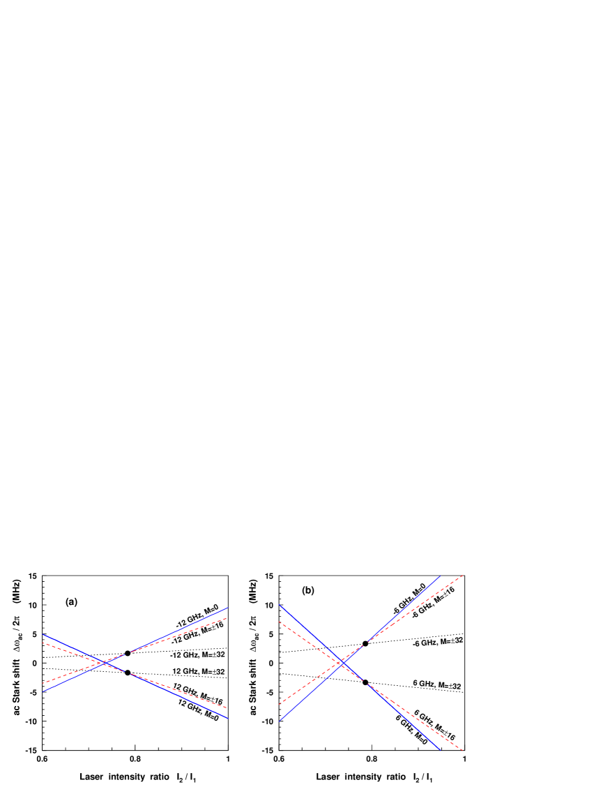
Figure 6: The ac Stark shift in the $\overline{p}{\rm{}^{4}He}^{+}$ resonance $(36,34)$$\rightarrow$$(34,32)$ estimated from the state polarizabilities $\alpha_{s}$ and $\alpha_{t}$, as a function of the intensity ratio $I_{2}/I_{1}$ between the two laser beams with $I_{1}$ fixed at $5\times 10^{4}$ W/cm². The shift for transitions involving states involving the magnetic substates $M=0$, $\pm 16$, and $\pm 32$ are indicated. The virtual intermediate state is tuned $\Delta\omega_{d}/2\pi=\pm 12$ GHz (a) and $\pm 6$ GHz (b) from the real state.

In Fig. 6 (a), the ac Stark shift $\Delta\omega_{\rm ac}/2\pi$ for $M$-values $0$, $\pm 16$, and $\pm 32$, and two laser offsets $\Delta\omega_{d}/2\pi=-12$ and 12 GHz obtained from the above equations are plotted as a function of the intensity ratio $I_{2}/I_{1}=F_{2}^{2}/F_{1}^{2}$ between the two laser beams. Here $I_{1}$ fixed at $\sim 5\times 10^{4}$ W/cm² while $I_{2}$ is scanned between $(3-5)\times 10^{4}$ W/cm². We find a positive shift ($\Delta\omega_{\rm ac}>0$) at two combinations of laser offsets and intensities ($\Delta\omega_{d}>0$, $I_{1}\gg I_{2}$) and ($\Delta\omega_{d}<0$, $I_{1}\ll I_{2}$). Conversely the shift is negative $\Delta\omega_{\rm ac}<0$ at ($\Delta\omega_{d}<0$, $I_{1}\gg I_{2}$) and ($\Delta\omega_{d}>0$, $I_{1}\ll I_{2}$). In addition to the ac Stark shift, the tensor polarizabilities cause the resonance line to split depending on the $M$-value of the involved states. At conditions of $I_{2}/I_{1}<0.6$ or $>1$ the ac Stark shift and splitting can reach values of more than 5–10 MHz. At smaller offsets $\Delta\omega_{d}/2\pi=\pm 6$ GHz, the ac Stark shift and splitting become twice as large [Fig. 6 (b)].

The ac Stark shift arising from $\alpha_{s}$ and the splitting due to $\alpha_{t}$ can be minimized by adjusting the laser intensities to the values indicated by filled circles in Figs. 6 (a)–(b),

$$\frac{I_{2}}{I_{1}}\sim\frac{\alpha_{s}(\omega_{1})_{(34,32)}}{\alpha_{s}(\omega_{2})_{(36,34)}}\sim 0.76.$$ (17)

An important point is that when the sign of the laser detuning is reversed, e.g., from $\Delta\omega_{d}/2\pi=-12$ to 12 GHz, the resulting ac Stark shift also reverses sign but its magnitude remains constant,

$$\Delta\omega_{\rm ac}(\omega_{1},\omega_{2})=-\Delta\omega_{\rm ac}(\omega_{1}-2\Delta\omega_{d},\omega_{2}+2\Delta\omega_{d}).$$ (18)

This means that the residual ac Stark shift can be canceled by comparing the two-photon transition frequencies measured at laser offsets of opposite sign but the same absolute value, i.e., $\Delta\omega_{d}$ and $-\Delta\omega_{d}$.

Fig. 7 shows the ac Stark shifts and transition amplitudes $\kappa_{L,L-2,M}$ of all magnetic sublines between $M=-32$ and $32$ of this two-photon resonance at laser offsets $\Delta\omega_{d}/2\pi=12$ GHz (a)–(c) and $-12$ GHz (d)–(f). The profiles were calculated at three ratios of the laser intensities $I_{2}/I_{1}=0.6$, 0.78, and 1.0 with $I_{1}$ fixed at $5\times 10^{4}$ W/cm². The ac Stark effect causes a triangular profile with the $M=0$ transitions being strongest and shifting the most. In actual experiments involving pulsed laser beams, these shifts and splittings will smear out due to nanosecond-scale changes in the light field intensities $I_{1}(t)$ and $I_{2}(t)$.

III.5 Hyperfine structure

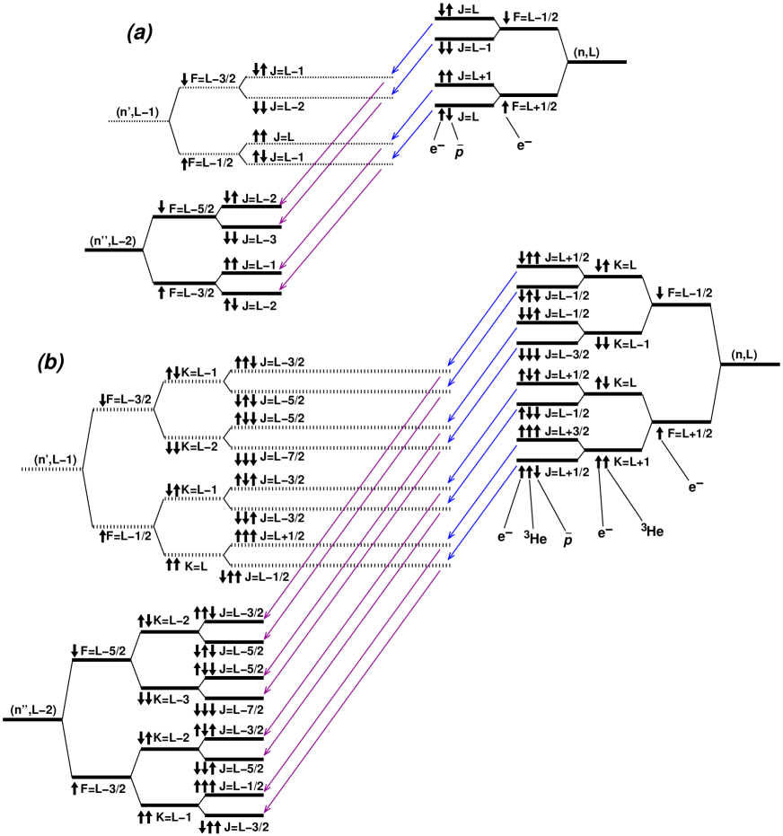
Figure 8: Energy level diagram showing the hyperfine sublevels of the resonance parent, intermediate, and daughter states involved in the two-photon transitions of $\overline{p}{\rm{}^{4}He}^{+}$ (a). The spin orientation $(S_{e},S_{\overline{p}})$ of each hyperfine sublevel is indicated by arrows. The four strongest two-photon transitions are indicated with solid arrows. The same figure in the case of $\overline{p}{\rm{}^{3}He}^{+}$, showing the eight strong lines between hyperfine levels $(S_{e},S_{h},S_{\overline{p}})$, see text.

We next study the hyperfine lines that appear in the two-photon resonance profile. The hyperfine substates of the parent, intermediate, and daughter states $(n,L)$, $(n-1,L-1)$, and $(n-2,L-2)$ in $\overline{p}{\rm{}^{4}He}^{+}$ are shown schematically in Fig. 8 (a). Due to the dominant interaction between the electron spin $\mathbf{S}_{e}$ and the antiproton orbital angular momentum $\mathbf{L}$, a pair of fine structure sublevels of intermediate angular momentum quantum number $F=L\pm 1/2$ and a splitting 10–15 GHz arise. The interactions involving the antiproton spin $\mathbf{S}_{\overline{p}}$ cause each fine structure sublevel to split by a few hundred MHz into pairs of hyperfine sublevels of total angular momentum quantum number $J=F\pm 1/2$. In Fig. 8 (a), the spin orientations of the electron and antiproton $(S_{e},S_{\overline{p}})$ are indicated for the four hyperfine sublevels. For example the energetically highest-lying component consists of a spin-down electron and spin-up antiproton, i.e. $(S_{e},S_{\overline{p}})=(\downarrow\uparrow)$.

In the $\overline{p}{\rm{}^{3}He}^{+}$ case [Fig. 8 (b)], the electronic fine structure sublevels of $F=L\pm 1/2$ are similarly split by $\sim\!10$ GHz. Each fine structure sublevel is then split into pairs of ³He hyperfine sublevels of intermediate angular momentum $K=F\pm\frac{1}{2}$ arising from the interactions involving the nuclear spin $\mathbf{S}_{h}$. The antiproton spin gives rise to eight hyperfine sublevels of total angular momentum $J=K\pm\frac{1}{2}$. The spin orientations of the three constituent particles $(S_{e},S_{h},S_{\overline{p}})$ are indicated for each substate in Fig. 8 (b).

In Fig. 8 (a)–(b), the four and eight strongest two-photon transitions between the hyperfine sublevels of $\overline{p}{\rm{}^{4}He}^{+}$ and $\overline{p}{\rm{}^{3}He}^{+}$ are indicated by arrows. These transitions pass through the virtual intermediate state without flipping the spin of any constituent particle. Many other transitions are possible, but they all involve spin-flip and so their amplitudes are suppressed by three orders of magnitude or more.

III.6 Optical rate equations

To simulate $\overline{p}{\rm He}^{+}$ two-photon resonance profiles, we used the following nonlinear rate equations which describe a three-level model,

$$\begin{array}[]{@{}l}\displaystyle\frac{\partial\rho_{aa}}{\partial t}=-{\rm Im}(\Omega_{1M}\rho_{ab}),\\[11.38109pt] \displaystyle\frac{\partial\rho_{bb}}{\partial t}={\rm Im}(\Omega_{1M}\rho_{ab})-{\rm Im}(\Omega_{2M}\rho_{bc}),\\[11.38109pt] \displaystyle\frac{\partial\rho_{cc}}{\partial t}=-\gamma_{c}\rho_{cc}+{\rm Im}(\Omega_{2M}\rho_{bc}),\\[11.38109pt] \displaystyle\frac{\partial\rho_{ab}}{\partial t}=-id_{ab}\rho_{ab}+i\frac{\Omega_{1M}}{2}(\rho_{aa}-\rho_{bb})+i\frac{\Omega_{2M}}{2}\rho_{ac},\\[11.38109pt] \displaystyle\frac{\partial\rho_{bc}}{\partial t}=-id_{bc}\rho_{bc}+i\frac{\Omega_{2M}}{2}(\rho_{bb}-\rho_{cc})-i\frac{\Omega_{1M}}{2}\rho_{ac},\\[11.38109pt] \displaystyle\frac{\partial\rho_{ab}}{\partial t}=-id_{ac}\rho_{ac}+i\frac{\Omega_{2M}}{2}\rho_{aa}-i\frac{\Omega_{1M}}{2}\rho_{bc}.\end{array}$$ (19)

Here the density matrix $\rho_{aa}$, $\rho_{bb}$, and $\rho_{cc}$ represent the antiproton populations in the parent, intermediate, and daughter states. The mixing between pairs of states induced by the lasers are denoted by $\rho_{ab}$, $\rho_{bc}$, and $\rho_{ac}$, the Auger decay rate of the daughter state by $\gamma_{c}$. The three detunings that appear in Eq. 19 can be calculated using the equations,

$$\begin{array}[]{@{}l}\displaystyle d_{ab}=E_{b}-E_{a}-\left(1+\frac{v_{z}}{c}\right)\omega_{1}-i\frac{\gamma_{a}+\gamma_{b}}{2},\\[11.38109pt] \displaystyle d_{bc}=E_{c}-E_{b}-\left(1-\frac{v_{z}}{c}\right)\omega_{2}-i\frac{\gamma_{b}+\gamma_{c}}{2},\\[11.38109pt] \displaystyle d_{ac}=E_{c}-E_{a}-\left(1+\frac{v_{z}}{c}\right)\omega_{1}-\left(1-\frac{v_{z}}{c}\right)\omega_{2}-i\frac{\gamma_{a}+\gamma_{c}}{2},\end{array}$$ (20)

where $v_{z}$ denotes the velocity component of the atom in the direction of the $\omega_{1}$-laser beam, $E_{a}$, $E_{b}$, and $E_{c}$ the binding energy of the hyperfine states involved in the transition, and $\gamma_{a}$ and $\gamma_{b}$ the radiative rates of the parent and intermediate states. The angular Rabi frequencies of single-photon transitions induced between the parent and intermediate states of magnetic quantum number $M$, and the intermediate and daughter states are respectively denoted by $\Omega_{1M}$ and $\Omega_{2M}$.

Values of $\Omega_{1M}/2\pi$ (in s^-1) for the transition $(0,L,F,K,J,M)$$\rightarrow$$(q,L\!-\!1,F^{\prime},K^{\prime},J^{\prime},M)$ in $\overline{p}{\rm{}^{3}He}^{+}$ by linearly-polarized laser light of intensity $I_{1}$ (in W/cm²) can be calculated,

$$\begin{array}[]{@{}l}\displaystyle\Omega_{1M}(\rm S.I.)=\sqrt{\frac{2I_{1}}{\epsilon_{0}c}}\frac{ea_{0}}{h}\\[11.38109pt] \displaystyle\hskip 17.07164pt\times\Bigl{|}\langle 0LFKJM|\mathbf{d}|q(L\!-\!1)F^{\prime}K^{\prime}J^{\prime}M\rangle\Bigr{|}\ (\rm a.u.)\end{array}$$ (21)

where the transition matrix element (in atomic units) can be derived using the Wigner $3j$- and $6j$-symbols,

$$\begin{array}[]{@{}l}\displaystyle\Bigl{|}\langle\,0LFKJM|\,\mathbf{d}\,|q(L\!-\!1)F^{\prime}K^{\prime}J^{\prime}M\,\rangle\Bigr{|}\\[11.38109pt] \displaystyle=\,\vrule width=0.7pt,height=19.0pt,depth=13.0pt\langle\,0L\|\mathbf{d}\|q(L\!-\!1)\,\rangle\left(\begin{array}[]{@{\,}c@{\;\;}c@{\;\;}c@{\,}}J&1&J^{\prime}\\ M&0&-M\end{array}\right)\\[11.38109pt] \displaystyle\hskip 28.45274pt\times\sqrt{(2J\!+\!1)(2J^{\prime}\!+\!1)}\>\left\{\begin{array}[]{@{\,}ccc@{\,}}K^{\prime}&J^{\prime}&\frac{1}{2}\\ J&K&1\end{array}\right\}\\[11.38109pt] \displaystyle\hskip 28.45274pt\times\sqrt{(2K\!+\!1)(2K^{\prime}\!+\!1)}\left\{\begin{array}[]{@{\,}ccc@{\,}}F^{\prime}&K^{\prime}&\frac{1}{2}\\ K&F&1\end{array}\right\}\\[11.38109pt] \displaystyle\hskip 28.45274pt\times\sqrt{(2F\!+\!1)(2F^{\prime}\!+\!1)}\>\left\{\begin{array}[]{@{\,}ccc@{\,}}L^{\prime}&F^{\prime}&\frac{1}{2}\\ F&L&1\end{array}\right\}\,\vrule width=0.7pt,height=19.0pt,depth=13.0pt\,.\end{array}$$ (22)

Eq. (22) only provides approximate values for the transition matrix elements since $L$, $F$, and $K$ are not exact quantum numbers of the three-body Hamiltonian. The results however agree well with exact transition amplitudes within $1\%$ accuracy.

We assume that the $\overline{p}{\rm He}^{+}$ $M$-states are uniformly populated in the parent state and follow a Maxwellian thermal distribution with $T\!\sim\!10$ K. We integrate Eq. (19) to simulate the antiprotons depopulated by the two laser beams into the daughter state producing the spectroscopic signal. The laser pulses are assumed to have Gaussian temporal profiles of pulse length $\Delta t=100$ ns.

Fig. 9 (a)–(b) shows the efficiency $\varepsilon$ of the laser pulses depleting the population in the parent state of the two-photon transition $(36,34)$$\rightarrow$$(34,32)$ of $\overline{p}{\rm{}^{4}He}^{+}$ [i.e. $\varepsilon=1$ if the laser induces all the antiprotons occupying state $(n,L)$ to annihilate, and $\varepsilon=0$ when no such annihilations occur]. The virtual intermediate state is offset $\omega_{d}/2\pi=-12$ GHz away from state $(35,33)$, so that $\omega_{1}+\omega_{2}$ coincides with the hyperfine component $(S_{e},S_{\overline{p}})=(\uparrow\uparrow)$$\rightarrow$$(\uparrow\uparrow)$ of the resonance line. As the laser intensity is increased between $p=0$ and $0.2$ mJ/cm², the $\varepsilon$-value increases quadratically as expected for a two-photon process. It begins to saturate at $p>1$ mJ/cm² corresponding to $\varepsilon\sim 0.3$. Monte Carlo simulations indicate that the two-photon resonance signal corresponding to $\varepsilon\sim 0.3$ would be strong enough for clear detection against the background caused by spontaneously annihilating antiprotons horinim with a signal-to-noise ratio of $>5$. Higher laser intensities would of course provide an even stronger signal, but power broadening effects then deteriorate the spectral resolution to several hundred MHz and so this should be avoided for high-precision spectroscopy.

The resonance profiles of the two-photon transitions $(40,36)\rightarrow(38,34)$ of the $v=3$ cascade, $(38,35)\rightarrow(36,33)$ of $v=2$, $(36,34)\rightarrow(34,32)$ of $v=1$, and $(33,32)\rightarrow(31,30)$ of $v=0$ in $\overline{p}{\rm{}^{4}He}^{+}$ at temperature $T\sim 10$ K are shown in Figs. 10 (a)–(d). These resonances have among the largest transition amplitudes, and the Auger decay rates of the daughter states are large $\gamma_{A}=(2.5-4)\times 10^{8}$ s^-1 which is a necessary condition to obtain a strong annihilation signal horinim . The intensities of the two lasers are around $p\sim 1$ mJ/cm². The laser frequency $\omega_{1}$ is fixed to an offset corresponding to $\Delta\omega_{d}/2\pi=-12$ GHz from the intermediate state, whereas $\omega_{2}$ was scanned between -0.9 and 0.9 GHz around the two-photon resonance defined by $\omega_{1}+\omega_{2}$. In each simulated profile, the positions of the four hyperfine lines are indicated with arrows together with the corresponding spin orientations $(S_{e},S_{\overline{p}})$. The $\sim 200$ MHz linewidth of these profiles are primarily caused by the large Auger width of the daughter states, and the residual Doppler and power broadening.

The resonance $(40,36)$$\rightarrow$$(38,34)$ shows a two-peak structure [Fig. 10 (a)] with a frequency interval of $\sim 1.1$ GHz which arises from the dominant spin-orbit interaction between $\mathbf{S}_{e}$ and $\mathbf{L}$. Each peak is a superposition of two hyperfine lines with a few tens of MHz spacing caused by a further interaction between the antiproton and electron spins. The asymmetric structure of the profile of Fig. 10 (a) is due to the fact that the 25-MHz spacing between the hyperfine lines $(S_{e},S_{\overline{p}})=(\uparrow\uparrow)$$\rightarrow$$(\uparrow\uparrow)$ and $(\uparrow\downarrow)$$\rightarrow$$(\uparrow\downarrow)$ are small compared to the 75-MHz spacing between $(\downarrow\uparrow)$$\rightarrow$$(\downarrow\uparrow)$ and $(\downarrow\downarrow)$$\rightarrow$$(\downarrow\downarrow)$ The spacings between the hyperfine lines becomes gradually smaller for lower-lying transitions involving states of smaller $n$- and $v$-values, e.g., $0.8$ and $0.5$ GHz for $(38,35)$$\rightarrow$$(36,33)$ and $(36,34)$$\rightarrow$$(34,32)$. The hyperfine lines can no longer be resolved for the lowest$-n$ transition $(33,32)$$\rightarrow$$(31,30)$ [Fig. 12 (d)]. The low transition probability (Table 1) of this resonance causes the small depopulation efficiency $\varepsilon<0.1$ seen here; laser intensities of $p\geq 2$ mJ/cm² would be needed to produce a sufficient experimental signal.

We expect the two UV transitions $(n,L)=(36,34)$$\rightarrow$$(34,32)$ and $(33,32)$$\rightarrow$$(31,30)$ in $\overline{p}{\rm{}^{4}He}^{+}$ to yield the highest signal-to-noise ratios in laser spectroscopy experiments. This is because the parent states $(36,34)$ and $(33,32)$ retain large antiproton populations for long periods $t=3$–10 $\mu{\rm s}$ following $\overline{p}{\rm He}^{+}$ formation mhori2002 . By comparison, cascade processes rapidly deplete the populations in higher $n>37$ states within $1$-2 $\mu{\rm s}$, and so the associated two-photon spectroscopy signals contain a large background due to the spontaneously annihilating $\overline{p}{\rm He}^{+}$ atoms mhori2002 ; mhori2004 .

Higher experimental precisions on $\nu_{\rm exp}$ may be achieved by cooling the atoms to lower temperature and by inducing two-photon transitions between pairs of $\overline{p}{\rm He}^{+}$ states with microsecond-scale lifetimes. Fig. 10 (e) shows the resonance $(37,35)$$\rightarrow$$(35,33)$ of $\overline{p}{\rm{}^{4}He}^{+}$ at temperature $T=1.5$ K. Both parent and daughter states have lifetimes of $\tau\sim 1$ $\mu{\rm s}$, and so its natural linewidth $\sim 200$ kHz is two orders of magnitude smaller than in the other resonances Fig. 10 (a)–(d) studied here. It is unfortunately difficult to measure this transition experimentally, as the present detection method requires the daughter state to proceed rapidly to antiproton annihilation.

The profiles of two $\overline{p}{\rm{}^{3}He}^{+}$ resonances which are expected to yield the highest signal to noise ratios mhori2002 $(35,33)$$\rightarrow$$(33,31)$ and $(33,32)$$\rightarrow$$(31,30)$ at temperature $T\sim 10$ K are shown in Fig. 11 (a)–(b). The positions of the eight hyperfine lines and their spin configurations $(S_{e},S_{h},S_{\overline{p}})$ are indicated by arrows. Due to the large number of partially overlapping lines, it may be difficult to determine the $\nu_{\rm exp}$-values for $\overline{p}{\rm{}^{3}He}^{+}$ with a similar level of precision as in $\overline{p}{\rm{}^{4}He}^{+}$. The problem would be especially acute in the case of $(33,32)$$\rightarrow$$(31,30)$ [Fig. 11 (b)] which contain 8 sublines within a relatively small 0.6-GHz interval.

We finally use these numerical simulations to determine the ac Stark shift under realistic experimental conditions. Fig. 12 (a) shows the profiles of the resonance $(36,34)$$\rightarrow$$(34,32)$ of $\overline{p}{\rm{}^{4}He}^{+}$ at temperature $T\!\sim\!10$ K and laser offset $\Delta\omega_{d}/2\pi\!=\!-12$ GHz. They were calculated at two combinations of the laser intensities: $I_{1}=5\!\times\!10^{4}$ W/cm² and $I_{2}=2.5\!\times\!10^{4}$ W/cm² (broken lines) and $I_{1}\!=\!I_{2}\!=\!5\!\times\!10^{4}$ W/cm² (solid lines). As $I_{2}/I_{1}$ is increased, the transition frequency shifts to larger values. In Fig. 12 (b), the ac Stark shifts $\Delta\omega_{\rm ac}/2\pi$ determined from the simulated profiles of Fig. 12 (a) at laser offsets $\Delta\omega_{d}/2\pi=-12$ GHz are plotted using filled circles. It increases linearly from $-2$ MHz at $I_{2}/I_{1}=0.5$, to 5 MHz at $I_{2}/I_{1}=1$. A similar plot for offset $\Delta\omega_{d}/2\pi=12$ GHz is shown using filled squares. The two calculated sets of ac Stark shifts are of equal magnitude and opposite sign, the minimum occurring around $I_{2}/I_{1}\sim 0.65$.

IV Conclusions

We conclude that two-photon transitions in $\overline{p}{\rm He}^{+}$ of the type $(n,L)$$\rightarrow$$(n\!-\!2,L\!-\!2)$ can indeed be induced using two counterpropagating nanosecond laser pulses of intensity $\sim 1$ mJ/cm², for cases wherein the virtual intermediate state is tuned within $\left|\Delta\omega_{d}/2\pi\right|=10$–20 GHz of the real state $(n\!-\!1,L\!-\!1)$. The spectral resolution of the measured resonances should increase by an order of magnitude or more compared to conventional single-photon spectroscopy. The ac Stark shifts at these experimental conditions can reach several MHz or more, but this can be minimized by carefully adjusting the relative intensities of the two laser beams. Any remaining shift can be canceled by comparing the resonance profiles measured at positive and negative offsets $\pm\Delta\omega_{d}$ of the virtual intermediate state from the real state. In practice, this can be done by, e.g., using a frequency comb udem to accurately control the frequencies $\omega_{1}$ and $\omega_{2}$ of the counterpropagating laser beams. The UV two-photon transitions $(36,34)$$\rightarrow$$(34,32)$ and $(33,32)$$\rightarrow$$(31,30)$ in $\overline{p}{\rm{}^{4}He}^{+}$, and $(35,33)$$\rightarrow$$(33,31)$ in $\overline{p}{\rm{}^{3}He}^{+}$ are expected to yield particularly strong resonance signals that can be precisely measured.

Table 1: Some single-photon transitions in $\overline{p}{\rm{}^{4}He}^{+}$ and $\overline{p}{\rm{}^{3}He}^{+}$: their vibrational quantum number $v$, transition frequency, and absolute value of the transition matrix element (i.e. dipole moment).

$(n,L)\rightarrow(n^{\prime},L^{\prime})$	$v$	Trans. freq.	Dipole moment	Rad. rate
		(THz)	(a.u.)	($10^{5}$ ${\rm s}^{-1}$)
$\overline{p}{\rm{}^{4}He}^{+}$ states
$(40,36)\rightarrow(39,35)$	3	444.8	2.28	4.71
$(39,35)\rightarrow(38,34)$	3	501.9	2.02	5.44
$(38,35)\rightarrow(37,34)$	2	566.1	1.82	6.36
$(37,34)\rightarrow(36,33)$	2	636.9	1.58	7.01
$(37,35)\rightarrow(36,34)$	1	638.6	1.61	7.15
$(36,34)\rightarrow(35,33)$	1	717.5	1.38	7.63
$(35,33)\rightarrow(34,32)$	1	804.6	1.16	7.92
$(33,32)\rightarrow(32,31)$	0	1012.4	0.79	7.42
$(32,31)\rightarrow(31,30)$	0	1132.6	0.62	6.62
$\overline{p}{\rm{}^{3}He}^{+}$ states
$(39,35)\rightarrow(38,34)$	3	445.8	2.30	4.96
$(38,34)\rightarrow(37,33)$	3	505.2	2.03	5.77
$(37,34)\rightarrow(36,33)$	2	572.0	1.83	6.81
$(36,33)\rightarrow(35,32)$	2	646.2	1.58	7.55
$(35,33)\rightarrow(34,32)$	1	730.8	1.37	8.27
$(34,32)\rightarrow(33,31)$	1	822.8	1.15	8.59
$(33,32)\rightarrow(32,31)$	0	928.8	0.95	8.44
$(32,31)\rightarrow(31,30)$	0	1043.1	0.77	7.94

Table 2: Scalar and tensor polarizabilities of the $\overline{p}{\rm{}^{4}He}^{+}$ states $(34,32)$ and $(36,34)$ at offset frequencies of the lasers between $\Delta\omega_{d}/2\pi=-100$ and 100 GHz, see text.

	Polarizabilities (a.u.)
$\Delta\omega_{d}/2\pi$	$-100$ GHz	$-12$ GHz	$-6$ GHz	6 GHz	12 GHz	100 GHz
$(n,L)=(36,34)$ state
$\alpha_{s}(\omega_{2})_{(36,34)}$	$-602$	$-5.02\times 10^{3}$	$-1.00\times 10^{4}$	$1.00\times 10^{4}$	$5.02\times 10^{3}$	$602$
$\alpha_{s}(\omega_{1})_{(36,34)}$	$-1.61$	$-1.61$	$-1.61$	$-1.61$	$-1.61$	$-1.61$
$\alpha_{t}(\omega_{2})_{(36,34)}$	$601$	$5.02\times 10^{3}$	$1.00\times 10^{4}$	$-1.00\times 10^{4}$	$-5.02\times 10^{3}$	$-603$
$\alpha_{t}(\omega_{1})_{(36,34)}$	$0.204$	$0.203$	$0.203$	$0.203$	$0.203$	$0.203$
$\beta_{s}(\omega_{2})_{(36,34)}$	$-0.403$	$-0.401$	$-0.401$	$-0.401$	$-0.401$	$-0.400$
$\beta_{t}(\omega_{2})_{(36,34)}$	$-0.945$	$-0.946$	$-0.946$	$-0.947$	$-0.947$	$-0.948$
$(n,L)=(34,32)$ state
$\alpha_{s}(\omega_{2})_{(34,32)}$	$-2.06$	$-2.06$	$-2.06$	$-2.06$	$-2.06$	$-2.06$
$\alpha_{s}(\omega_{1})_{(34,32)}$	$-459$	$-3.81\times 10^{3}$	$-7.62\times 10^{3}$	$7.62\times 10^{3}$	$3.81\times 10^{3}$	$456$
$\alpha_{t}(\omega_{2})_{(34,32)}$	$0.265$	$0.265$	$0.265$	$0.265$	$0.265$	$0.264$
$\alpha_{t}(\omega_{1})_{(34,32)}$	$416$	$3.47\times 10^{3}$	$6.94\times 10^{3}$	$-6.95\times 10^{3}$	$-3.48\times 10^{3}$	$-417$
$\beta_{s}(\omega_{1})_{(34,32)}$	$-1.36$	$-1.36$	$-1.36$	$-1.36$	$-1.36$	$-1.36$
$\beta_{t}(\omega_{1})_{(34,32)}$	$-0.401$	$-0.401$	$-0.401$	$-0.401$	$-0.402$	$-0.402$

Figure 1: Energy level diagram indicating the two-photon transition $(n,L)=(36,34)$$\rightarrow$$(34,32)$ in $\overline{p}{\rm{}^{4}He}^{+}$. The relative position of the virtual intermediate state for a detuning frequency $\Delta\omega_{d}$ of the two counter-propagating laser beams are shown.

Figure 3: Transition matrix element of the two-photon resonance $(n,L)=(36,34)$$\rightarrow$$(34,32)$ as a function of the offset $\Delta\omega_{d}/2\pi$ of the two laser beams from the virtual intermediate state. The matrix element is averaged over the magnetic quantum number $M$. The arrow indicates the position wherein the two laser beams have equal frequencies.

Figure 4: Scalar dipole polarizability of states $(n,L)=(34,32)$ and $(36,34)$ versus frequency offset $\Delta\omega_{d}/2\pi$ of the virtual intermediate state from the real state $(35,33)$: $\alpha_{s}(w_{1})_{(34,32)}$ and $\alpha_{s}(w_{2})_{(36,34)}$ as defined in Eq. (5) (a)–(b). Tensor polarizabilities $\alpha_{t}(w_{1})_{(34,32)}$ and $\alpha_{t}(w_{2})_{(36,34)}$ (c)–(d).

Figure 5: Residual scalar dipole polarizability of states $(n,L)=(34,32)$ and $(36,34)$ versus frequency offset $\Delta\omega_{d}/2\pi$ of the virtual intermediate state from the real state $(35,33)$: $\beta_{s}(\omega_{1})_{(34,32)}$ and $\beta_{s}(\omega_{1})_{(34,32)}$, and $\beta_{t}(\omega_{2})_{(36,34)}$ and $\beta_{t}(\omega_{2})_{(36,34)}$. The contributions of all states except the intermediate one $(35,33)$ are included.

Figure 7: Expected positions and intensities of the M-sublines of the two-photon transition $(36,34)$$\rightarrow$$(34,32)$ in $\overline{p}{\rm{}^{4}He}^{+}$, wherein the virtual intermediate state is offset $\Delta\omega_{d}/2\pi\sim 12$ GHz (a)–(c) and $-12$ GHz (d)–(f) from the state $(35,33)$. The intensity ratios $I_{2}/I_{1}$ between the two laser beams were varied between 0.6, 0.78, and 1.0 in each figure, whereas $I_{1}$ was kept constant at $\sim 5\times 10^{4}$ W/cm².

Figure 9: Depopulation efficiency of the two-photon transition $(n,L)=(36,34)$$\rightarrow$$(34,32)$ in $\overline{p}{\rm{}^{4}He}^{+}$ at various intensities of the two laser beams.

Figure 10: Simulated resonance profiles of five two-photon transitions in $\overline{p}{\rm{}^{4}He}^{+}$ excited at laser intensities $p=1$ mJ/cm². The virtual intermediate state was tuned $\Delta\omega_{d}/2\pi\sim-12$ GHz from a real state. The positions of the four hyperfine lines are indicated by arrows, together with the principal and angular momentum quantum numbers $(n,L)$ and spin orientations $(S_{e},S_{\overline{p}})\rightarrow(S^{\prime}_{e},S^{\prime}_{\overline{p}})$ of the resonance parent and daughter states.

Figure 11: Simulated resonance profiles of two two-photon transitions in $\overline{p}{\rm{}^{3}He}^{+}$ excited at laser intensities $p=1$ mJ/cm². The virtual intermediate state was tuned $\Delta\omega_{d}/2\pi\sim-12$ GHz from a real state. The positions of the eight hyperfine lines are indicated by arrows, together with the principal and angular momentum quantum numbers $(n,L)$ and spin orientations $(S_{e},S_{h},S_{\overline{p}})$$\rightarrow$$(S^{\prime}_{e},S^{\prime}_{h},S^{\prime}_{\overline{p}})$ of the resonance parent and daughter states.

Figure 12: Simulated profiles of the resonance $(n,L)=(36,34)$$\rightarrow$$(34,32)$ in $\overline{p}{\rm{}^{4}He}^{+}$, with the frequency offset $\Delta\omega_{d}/2\pi\sim-12$ GHz and intensity ratio between the two lasers $I_{2}/I_{1}=0.5$ (dashed lines) and 1 (solid lines) for constant $I_{1}\sim 5\times 10^{4}$ W/cm² (a). The ac Stark shift in the simulated profiles for offsets $\Delta\omega_{d}/2\pi\sim-12$ GHz (solid circles) and $12$ GHz (squares), as a function of $I_{2}/I_{1}$.