Direct Wolf summation of a polarizable force field for silica

Abstract

We extend the Wolf direct, pairwise $r^{-1}$ summation method with spherical truncation to dipolar interactions in silica. The Tangney-Scandolo interatomic force field for silica takes regard of polarizable oxygen atoms whose dipole moments are determined by iteration to a self-consistent solution. With Wolf summation, the computational effort scales linearly in the system size and can easily be distributed among many processors, thus making large-scale simulations of dipoles possible. The details of the implementation are explained. The approach is validated by estimations of the error term and simulations of microstructural and thermodynamic properties of silica.

Copyright (2010) American Institute of Physics. This article may be downloaded for personal use only. Any other use requires prior permission of the author and the American Institute of Physics.

I Introduction

Silica is by far the most abundant mineral in the earth’s crustIler (1979). This makes it an interesting system to study in simulation. Additionally, SiO₂ shows a wide range of crystalline structures depending on temperature and pressure, and it can also be solidified as a glass. Although there have been enormous advances in ab initio simulations of silicaKarki et al. (2007), many effects are inaccessible due to length and time scale restrictions of these models. For large-scale atomistic simulations, a high-quality model of the interactions, a so-called effective potential or force field, is essential.

Many attempts to parameterize the interactions in silica have been made in the past thirty years, with various levels of computational intensity and accuracy. Some of the earlier potentials are still widely used, like for example the potential of van Beest, Kramer, and van Santen (BKS) van Beest et al. (1990), a pure pair potential with fixed charges and short-range corrections. However, it is believed that many-body effects are important for correctly describing bond angles and bond-bending vibration frequencies in network-forming glasses like SiO₂.Wilson et al. (1996); Wilson and Walsh (2000) The potential model of Tangney and ScandoloTangney and Scandolo (2002) (TS) treats the oxygen atoms as polarizable. The dipole moments of these atoms are determined self-consistently from the local electric field, with short-range corrections to the polarization.Rowley et al. (1998) A more detailed description of the TS potential is given in Sec. II.1.

A comparison of various silica force fields showedHerzbach et al. (2005) that the polarizable ion model of TS yields significantly better results for many properties compared to the BKS potential, while still leaving room for improvement. In a recent study by Paramore et al.Paramore et al. (2008), attempts to map the implicit many-body effects in the TS model to pure pairwise interactions did not lead to an accurate potential. This confirms that polarization effects are indeed necessary for a proper description of SiO₂.

In all potential models discussed above, the ions carry some charge $q_{i}$ and interact with a Coulomb potential. This leads to the classical Madelung problem:Madelung (1918) determining the energy of a condensed system with a pairwise $r^{-1}$ interaction. The convergence properties of the resulting sum require a special treatment, and a number of methods to evaluate the pairwise $r^{-1}$ sum have evolved, with the Ewald methodEwald (1921) as the best-known. There, rapid convergence for the total Coulomb energy of a set of $N$ ions with charge $q_{i}$ at positions $\bm{r}_{i}$ that are part of an infinite system of point charges,

$$E^{\text{tot}}=\frac{1}{2}\sum\limits_{i=1}^{N}\sum\limits_{j\neq i=1}^{\infty}\frac{q_{i}q_{j}}{r_{ij}},$$ (1)

(where $\bm{r}_{ij}=\bm{r}_{j}-\bm{r}_{i}$ and $r_{ij}=\left|\bm{r}_{ij}\right|$) is assured by a mathematical trick. Firstly, structural periodicity of linear size $L$ is artificially imposed on the system, and in the resulting expression a decomposition of unity of the form

$$1=\operatorname{erfc}\!\left(\kappa r\right)+\operatorname{erf}\!\left(\kappa r\right)$$ (2)

is inserted. The error function is defined as

$$\operatorname{erf}\!\left(\kappa r\right):=\frac{2}{\sqrt{\pi}}\int\limits_{0}^{\kappa r}\!dt\,e^{-t^{2}}.$$ (3)

The Ewald splitting parameter $\kappa$ controls the distribution of energy contributions between the two terms. Thus, Eq. (1) can be written as

$$\begin{split}E^{\text{tot}}=&\frac{1}{2}\sum\limits_{i=1}^{N}\sum\limits_{j=1}^{N}\sum\limits_{\bm{n}=\bm{0}}^{\infty}\,{}^{\prime}\frac{q_{i}q_{j}}{|\bm{r}_{ij}+\bm{n}L|}\left[\operatorname{erfc}(\kappa|\bm{r}_{ij}+\bm{n}L|)\right.\\ &\left.+\operatorname{erf}(\kappa|\bm{r}_{ij}+\bm{n}L|)\right],\end{split}$$ (4)

where the sum over periodic images $\bm{n}$ is primed to indicate that the $i=j$ term is to be omitted for $\bm{n}=\bm{0}$. Taking the Fourier transform of the error-function expression only, but not of the complementary error-function term, one can convert the conditionally convergent total energy Eq. (1) into the sum of real-space and reciprocal-space contributions $E_{\bm{r}}^{\text{tot}}$ and $E_{\bm{k}}^{\text{tot}}$ where each of these converges rapidly. The downside to the Ewald summation method is the scaling of the computational effort with the number of particles in the simulation box: Even when the balance between real- and reciprocal-space contributions controlled by $\kappa$ is optimized, the computational load increases at best as $O(N^{3/2})$.Fincham (1994) For large-scale simulations with millions of atoms, this is insufficient. Additionally, the Ewald technique is limited to periodic systems. In recent years, alternative simulation techniques that show better scaling properties have been developed, among them mesh-based methods or fast multipole methods.Gibbon and Sutmann (2002) The linear scaling, however, comes with considerable overhead. In contrast, Wolf et al.Wolf et al. (1999) proposed a direct summation technique with linear scaling ($O(N)$) for Coulomb interactions, that can easily be implemented in standard Molecular Dynamics (MD) codes. This so called Wolf summation takes into account the physical properties of the systems under study.

To this end, one looks at the Fourier transform of the error function term of Eq. (4)

$$E_{\bm{k}}^{\text{tot}}=\frac{2\pi}{L^{3}}\sum_{\bm{k}\neq\bm{0}}\sum_{i,j}q_{i}q_{j}e^{i\bm{k}\cdot(\bm{r}_{j}-\bm{r}_{i})}\frac{\exp(-\frac{|\bm{k}|^{2}}{4\kappa^{2}})}{|\bm{k}|^{2}}-\frac{\kappa}{\pi^{1/2}}\sum_{i}q_{i}^{2},$$ (5)

where the self term ($\bm{n}=\bm{0}$ and $i=j$) is now included in the summation and subtracted again separately. Eq. (5) can be rewritten as

$$E_{\bm{k}}^{\text{tot}} =\sum_{\begin{subarray}{c}\bm{k}\neq\bm{0}\\ |\bm{k}|<k_{c}\end{subarray}}S(k)\frac{\exp(-\frac{|\bm{k}|^{2}}{4\kappa^{2}})}{|\bm{k}|^{2}}-\frac{\kappa}{\pi^{1/2}}\sum_{i}q_{i}^{2},$$ (6)

where $$S(k) k=|\bm{k}|$$, with , is the charge structure factor

$$S(k) =\frac{2\pi}{L^{3}}\left|\sum_{j}q_{j}\exp(i\bm{k}\cdot\bm{r}_{j})\right|^{2}.$$ (7)

The charge structure factor is the Fourier transform of the charge-charge autocorrelation function.

In the systems of interest here, there are no long-range charge fluctuations; the charges form a cold dense plasma, screening each other. This means that for small wave vectors $k$, the charge structure factor is also small. If one now chooses a sufficiently small Ewald parameter $\kappa$, the reciprocal-space contribution can be neglected altogether. As $\kappa$ is linked to the real-space cut-off $r_{c}$, however, this might require a cut-off radius which is substantially larger than the range of traditional short-range interactions like in metals.

Concurrently, Wolf et al. also motivated a continuous and smooth cut-off of the remaining screened Coulomb potential $V(r_{ij})=q_{i}q_{j}\operatorname{erfc}(\kappa r_{ij})r_{ij}^{-1}$ at a cut-off radius $r_{c}$. The authors stated that shifting the pair potential so that it goes to zero smoothly at $r=r_{c}$ is equivalent to neutralizing the surface charge in a spherically truncated system. The strong fluctuations in the surface charge with varying $r_{c}$ inhibit the convergence to the true Madelung energy with increasing $r_{c}$. The combination of (i) shifting the potential so that it vanishes smoothly at the cut-off, and (ii) damping the Coulomb potential to reduce the required cut-off radius, but only so weakly that the reciprocal-space term can still be neglected, is called Wolf summation.

To evaluate the TS potential with the Wolf direct summation technique, one first has to extend the formalism to the treatment of dipolar interactions. How this is done is shown in Sec. II. We provide an estimate of the errors made by the approximation in Sec. III. The directly summed TS potential was implemented in the (limited range) MD code IMD,Stadler et al. (1997) and various observables were determined and compared to the original TS implementation with full Ewald summation (Sec. IV). Finally, we sum up the results in Sec V, where also an outlook is given.

II Wolf summation of dipole contributions

II.1 Tangney-Scandolo potential model

In the TSTangney and Scandolo (2002) force field, there are two contributions to the potential energy of a system: a pairwise potential of Morse-Stretch form, and the electrostatic interactions between charges and induced dipoles on the oxygen atoms. The dipole moments depend on the local electric field at the respective atomic sites, which in turn is determined by the arrangement of charges and dipoles. This implies that a self-consistent solution must be found.

Tangney and Scandolo propose an iterative solution for the dipole moments, so that the dipole moment $\bm{p}_{i}^{n}$ on atom $i$ in iteration step $n$ is

$$\bm{p}_{i}^{n}=\alpha\bm{E}(\bm{r}_{i};\{\bm{p}_{j}^{n-1}\}_{j=1,N},\{\bm{r}_{j}\}_{j=1,N})+\bm{p}_{i}^{\text{SR}},$$ (8)

where $\alpha$ is the polarizability of atom $i$ and $\bm{E}(\bm{r}_{i})$ the electric field at position $\bm{r}_{i}$, which is calculated from the dipole moments (and charges) in the previous iteration step. The short-range dipole moment $\bm{p}_{i}^{\text{SR}}$ is the contribution induced by short-range repulsive forces between anions and cations, that TS included following Rowley et al.Rowley et al. (1998) Starting from initial electric field strengths $\bm{E}^{0}(\bm{r})$ extrapolated from the previous three time steps, Eq. (8) is iterated until convergence is achieved for each MD time step.

The parameters of the TS potential were determined solely from ab initio results with the Force Matching methodErcolessi and Adams (1994). There, the potential is parameterized using first principles values of forces, stresses and energies in series of reference structures.

II.2 Smooth cut-off

For MD with limited-range interactions, the potentials and their first derivatives must go to zero continuously at a cut-off radius $r_{c}$; otherwise, atoms crossing this threshold might get unphysical kicks. For the Morse-Stretch pair potential, this is generally not problematic, as it decays with $r_{ij}$ fast enough. In MD, following Wolf et al.,Wolf et al. (1999) the potential $U_{\text{MS}}(r_{ij})$ is replaced by

$$\tilde{U}_{\text{MS}}(r_{ij})=U_{\text{MS}}(r_{ij})-U_{\text{MS}}(r_{c})-(r_{ij}-r_{c})U^{\prime}_{\text{MS}}(r_{c}),$$ (9)

where a prime denotes a derivative with respect to $r$.

The other functions used in the TS model have a general $r$ dependence of the form $r^{-n},n\in\{1,2,3\}$. Especially the Coulomb energy with its $r^{-1}$ dependency cannot simply be cut off without a treatment as in Eq. (9), for otherwise the energy of the system would fluctuate strongly with $r_{c}$, without convergence to the proper value. But even with a smooth cut-off (9), with which the Coulomb energy does converge, a rather large cut-off radius would be required to make shifting of the potential negligible. Fortunately, the Wolf direct summation methodWolf et al. (1999) includes a weak exponential damping of the Coulomb potential by $\operatorname{erfc}\!\left(\kappa r\right)$. Such a damped potential can be cut off smoothly at a much smaller radius $r_{c}$ without affecting the result. All integer powers of $r^{-1}$ are treated in a way to conserve the differential relationship between the functions, i.e. the damped functions are

$$r^{-1}\rightarrow r^{-1}\operatorname{erfc}(\kappa r)=:f_{-1}(r),$$ (10)

$$\begin{split}r^{-2}=-\frac{d(r^{-1})}{dr}\rightarrow&-\frac{d(r^{-1}\operatorname{erfc}(\kappa r))}{dr}\\ &=r^{-2}\operatorname{erfc}(\kappa r)-\frac{2\kappa\exp(-\kappa^{2}r^{2})}{\sqrt{\pi}r}\\ &=:f_{-2}(r).\end{split}$$ (11)

This procedure is also required to conserve the energy during an MD simulation, as discussed in more detail in Sec. II.3.

The damped potentials are then shifted to zero and zero derivative at the cut-off radius, as in (9). This allows for limited-range MD simulations with a standard MD code. The computational effort of such a simulation scales linearly in the number of particles (as the number of interactions that need to be evaluated per particle does not increase with the number of particles), but scales roughly with $O(r_{c}^{3})$.

II.3 Energy conservation

In MD simulations, the energy is conserved, if the forces on the particles are exactly equal to the gradient of the potential energy with respect to the atomic coordinates. Otherwise, the energy might oscillate or even drift off if not controlled by a thermostat. In standard MD simulations, the requirement is usually automatically fulfilled: The forces are calculated as the derivative of the potential, which depends directly on the atomic positions. In the TS model, there is also an indirect dependence, as the potential is also a function of the dipole moments:

$$U=U(\{\bm{r}_{i}\},\{\bm{p}_{i}(\{\bm{r}_{j}\})\}).$$ (12)

This would in principle lead to an extra contribution to the derivative of the potential,

$$\frac{dU}{d\{\bm{r}_{i}\}}=\frac{\partial U}{\partial\{\bm{r}_{i}\}}+\frac{\partial U}{\partial\{\bm{p}_{i}\}}\frac{\partial\{\bm{p}_{i}\}}{\partial\{\bm{r}_{j}\}},$$ (13)

which would be practically impossible to be determined effectively. Luckily, if the dipole moments are iterated until convergence is reached, we are at an extremal value of the potential energy, with $\partial U/\partial\{\bm{p}_{i}\}=0$, and so this part need not be evaluated. Imperfections in convergence may lead to a drift in the energy, however, as was already observed by Tangney and Scandolo.Tangney and Scandolo (2002)

When applying the Wolf formalism to the TS potential, another issue arises concerning the conservation of energy. It can most easily be explained with a simple one-dimensional example. Given are two oppositely charged point charges $\pm q$ at a mutual distance $r$. If the negatively charged one is polarizable with polarizability $\alpha$, it will get a dipole moment $p=\alpha q/(kr^{2})$, with $k=4\pi\epsilon_{0}$. This leads to a total interaction energy

$$U =\underbrace{-2\cdot\frac{1}{2}\frac{1}{k}\frac{q^{2}}{r}}_{q-q}-\underbrace{2\cdot\frac{1}{2}\frac{q}{k}\frac{p}{r^{2}}}_{q-p}+\underbrace{\frac{1}{2}\frac{p^{2}}{\alpha}}_{\text{dipole}},$$ (14)

from which it follows that

$$\frac{\partial U}{\partial p} =-\frac{1}{k}\frac{q}{r^{2}}+\underbrace{\frac{p}{\alpha}}_{=\frac{1}{k}\frac{q}{r^{2}}}=0.$$ (15)

Here, $q-q$ denotes the Coulomb interaction between charges, $q-p$ the interactions between charge and dipole, and the last term is the dipole energy. When we now damp and cut off the interactions, we replace the $r^{-1},r^{-2}$ functions by their damped and smoothed counterparts $\tilde{f}_{-1}(r),\tilde{f}_{-2}(r)$. If energy conservation is to be maintained, the differential relation between the $\tilde{f}_{-n}$ must be the same as for the $r^{-n}$:

$$\frac{d\tilde{f}_{-1}(r)}{dr}=-\tilde{f}_{-2}(r).$$ (16)

As a consequence, the first two derivatives of the smoothed damped Coulomb potential must be zero at $r_{c}$.

In MD simulation it is computationally advantageous to represent pair potential functions internally as functions of $r^{2}$, and their derivative as $f\hat{{}^{\prime}}:=r^{-1}df/dr$. The damped Coulomb potentials $f_{-1}$ and $r^{-1}f_{-2}(r)$ in their smoothly cut off version become

$$\begin{split}\tilde{f}_{-1}(r^{2})&=f_{-1}(r^{2})-f_{-1}(r_{c}^{2})\\ &\quad-\left.\tfrac{1}{2}f\hat{{}^{\prime}}_{-1}(r^{2})\right|_{r^{2}=r_{c}^{2}}(r^{2}-r_{c}^{2})\\ &\quad-\left.\tfrac{1}{8}f\hat{{}^{\prime}}\hat{{}^{\prime}}_{-1}(r^{2})\right|_{r^{2}=r_{c}^{2}}(r^{2}-r_{c}^{2})^{2}\end{split}$$ (17)

and

$$\begin{split}\quad\tfrac{1}{r}\tilde{f}_{-2}(r)&=\tfrac{1}{r}f_{-2}(r^{2})-\left.f\hat{{}^{\prime}}_{-1}(r^{2})\right|_{r^{2}=r_{c}^{2}}\\ &\quad-\left.\tfrac{1}{2}f\hat{{}^{\prime}}\hat{{}^{\prime}}_{-1}(r^{2})\right|_{r^{2}=r_{c}^{2}}(r^{2}-r_{c}^{2}).\end{split}$$ (18)

In this way, Wolf summation can be applied to dipolar interactions in the TS potential model. In Sec. III we will discuss why this approximation is physically justified.

II.4 Implementation

The ITAP Molecular Dynamics (IMD) packageStadler et al. (1997) is a flexible, highly scalable MD code for limited-range interactions, providing linear scaling up to thousands of CPUs. For finite-range interactions, the number of potential interaction partners of an atom is uniformly bounded. In order to reach linear scaling in the number of atoms, it is essential to find these interaction partners efficiently. IMD uses a combination of link-cells and neighbor lists, where the former are used to compute the latter in an efficient way. Since Wolf summation requires a relatively large cut-off radius, these neighbor list can get fairly big, but on today’s machines this is not a problem. Parallelization is done via a fixed geometric domain decomposition, where each CPU gets an equal block of material. For the force computation, atoms at the surface of a block are exchanged with the neighboring CPUs.

All potential functions used in IMD are tabulated, even if some of these functions may be specified by giving the parameters of an analytic formula. In that case, potential tables are constructed from the analytic formula in a pre-processing step. During the simulation loop, the functions are then evaluated by table lookup and interpolation. This has proven to be the most flexible and efficient scheme, allowing also for very complicated potential functions. For all potential functions depending on the radius, care is taken that they vanish smoothly at the cut-off radius, along with their first derivative.

In contrast to other interactions implemented in IMD, the TS potential requires a self-consistency loop within each time step, during which the dipole strengths of the oxygen atoms are determined. Before entering this loop, the “static” contributions $\bm{E}_{\text{stat}}$ to the on-site electric field caused by the charges of anions and cations, and the short-range dipole contributions $\bm{p}_{i}^{\text{SR}}$ are calculated and stored. For the “induced” part of the electric field $\bm{E}_{\text{ind}}$, which is generated by the oxygen dipoles, Eq. (8) is then iterated until convergence is achieved. The iteration starts from an extrapolation of the local electric field at the previous three MD time steps. To improve the convergence of Eq. (8), $\bm{E}_{\text{ind}}^{n}$ is modified after each iteration step $n$ to include a small part $c$ from the previous iteration,

$$\bm{E}_{\text{ind}}^{n}\rightarrow(1-c)\bm{E}_{\text{ind}}^{n}+c\,\bm{E}_{\text{ind}}^{n-1}.$$ (19)

This damps the self-consistency loop and thus suppresses overshooting the optimal solution and subsequent oscillations. For optimal performance, a value of $c=0.2$ was used.

Convergence is achieved, when the root mean square deviation of all Cartesian dipole moment components between two iterations is less than a user-specified tolerance (given in units of the dipole moment). While a larger tolerance will reduce the iteration steps to convergence, it will also introduce a larger error in the energy conservation, which might lead to a temperature drift in microcanonical simulations. In practice, a convergence limit smaller than $10^{-6}$ Å$e$ (with elementary charge $e$) will not lead to further improvement. With this tolerance, about five iterations steps are typically needed per MD step.

In a parallel simulation, each CPU deals with a block of material. For the parallel evaluation of the energies and forces, at each MD step the types and positions of atoms near the surface of a block are first communicated to the neighboring CPUs. Each CPU can then perform a part of the energy and forces computation locally. As each force is computed only once, certain force and energy contributions have then to be communicated back to the home CPU of the corresponding atom, where it is added up. This scheme is valid for all finite range interactions. Since only communication between neighboring CPUs is necessary, the scheme is highly scalable.

For the TS potential the procedure is very similar, except that now there are additional data to be communicated. In each step of the self-consistency loop for the induced dipoles, the electric fields and dipole moments of atoms at the surface must be distributed to the neighboring CPUs, and collected again after they have been updated. There are several additional communication steps for each MD step, but these are of the same kind as for other short-range interactions (to neighbor CPUs only), and the balance between communication and computation is not affected. For this reason, simulations with the TS potential will scale as well as with other short-range potentials.

III Convergence and Error Estimation

III.1 Formal Analysis

The total interaction energy of $N$ dipole moments $\bm{p}_{i}$ at positions $\bm{r}_{i}$ is given by the expression

$$E^{\text{tot}}=-\frac{1}{2}\sum\limits_{\genfrac{}{}{0.0pt}{}{i,j}{i\neq j}}^{N}\,\bm{p}^{t}_{i}\left(\bm{\nabla}\otimes\bm{\nabla}\right)\left(\frac{1}{r_{ij}}\right)\bm{p}_{j},$$ (20)

with $\bm{r}_{ij}:=\bm{r}_{i}-\bm{r}_{j}$ and $r_{ij}:=|\bm{r}_{ij}|$. Imposing structural periodicity and inserting a decomposition of unity of the form

$$1=\operatorname{erfc}\!\left(\kappa r\right)+\operatorname{erf}\!\left(\kappa r\right),$$ (2)

where $\kappa$ is again the Ewald splitting parameter, we can rewrite above equation as

$$E^{\text{tot}}=-\frac{1}{2}\sum\limits_{i,j}^{N}\sum\limits_{\bm{n}=\bm{0}}^{\infty}\text{${}^{\prime}$}\,\bm{p}^{t}_{i}\left(\bm{\nabla}\otimes\bm{\nabla}\right)\\ \cdot\left(\frac{\operatorname{erfc}\!\left(\kappa|\bm{r}_{ij}+\bm{n}L|\right)+\operatorname{erf}\!\left(\kappa|\bm{r}_{ij}+\bm{n}L|\right)}{|\bm{r}_{ij}+\bm{n}L|}\right)\bm{p}_{j}.$$ (21)

The total energy splits into a real- and a reciprocal-space part:

$$E^{\text{tot}}=E^{\text{tot}}_{\bm{r}}+E^{\text{tot}}_{\bm{k}}$$ (22)

Since we later intend to neglect the reciprocal-space term for the Wolf summation, we are interested in the contribution of $E^{\text{tot}}_{\bm{k}}$. For its $\bm{k}$-behavior we have to take the Fourier transform of

$$E^{\text{tot}}_{\bm{k}}=-\frac{1}{2}\sum\limits_{i,j}^{N}\sum\limits_{\bm{n}=\bm{0}}^{\infty}\,\bm{p}^{t}_{i}\left(\bm{\nabla}\otimes\bm{\nabla}\right)\left(\frac{\operatorname{erf}\!\left(\kappa|\bm{r}_{ij}+\bm{n}L|\right)}{|\bm{r}_{ij}+\bm{n}L|}\right)\bm{p}_{j}.$$ (23)

The prime has been omitted, since the self term (for $\bm{n}=\bm{0}$ and $i=j$) is now finite. Because of the three-dimensional periodicity the above expression can be expanded into a Fourier series:

$$\widetilde{E}^{\text{tot}}_{\bm{k}}=\frac{2\pi Ne^{2}}{V}\sum\limits_{\bm{k}\neq\bm{0}}^{\infty}\,\bm{k}^{t}\mathbf{\underline{Q}}(\bm{k})\bm{k}\;\dfrac{\exp\!\left(-k^{2}/4\kappa^{2}\right)}{k^{2}},$$ (24)

where $V$ is the volume of the simulation cell and $\mathbf{\underline{Q}}(\bm{k})$ the dipole structure factor

$$\mathbf{\underline{Q}}(\bm{k}):=\frac{1}{Ne^{2}}\sum\limits_{i,j}^{N}\,\bm{p}_{i}\otimes\bm{p}_{j}\,e^{i\bm{k}\cdot\bm{r}_{ij}},$$ (25)

with the normalization factor $1/\sqrt{Ne^{2}}$, where $e$ denotes the elementary charge. As we can see in Eq. (24), the large $\bm{k}$ contributions to $\widetilde{E}^{\text{tot}}_{\bm{k}}$ tend to zero rapidly, whereas the small $\bm{k}$ contributions are governed by the behavior of $\mathbf{\underline{Q}}(\bm{k})$, which is expected to vanish as $k\rightarrow 0$.

III.2 Discussion

To legitimate the neglecting of the reciprocal-space term for the Wolf summation we have simulated liquid silica with 4896 atoms, where we get no spontaneous polarization as a first result. The total dipole moment is $p=6.76\cdot 10^{-29}$  Cm, which is insignificantly small compared to a fully polarized system and thus can be taken as a fluctuation. All values which are calculated in the course of the simulation are time-averaged over the full simulation time of one picosecond.

To analyze the $k\rightarrow 0$ behavior we calculated the dipole structure scalar,

$$Q(k)=\langle\bm{k}^{t}\mathbf{\underline{Q}}(\bm{k})\bm{k}\ \rangle_{S},$$ (26)

where the angular brackets indicate an average over a spherical shell $S$ with width $\Delta k$ centered at constant $|\bm{k}|=k$. Note that for a for a periodic system $\mathbf{\underline{Q}}$ is not a continuous function, but a discrete set, consisting of all reciprocal space vectors. Hence the average over the spherical shell is necessary. Fig. 1 shows the dipole structure scalar in liquid silica simulations. For small absolute values of $k$, $Q(k)$ goes to zero.

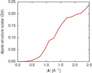
Figure 1: $k$-dependence of the dipole structure scalar $Q(k)$. For small $k$, the dipole structure factor is negligible.

Fig. 2 shows the $k$-dependence of the reciprocal-space term,

$$\widetilde{E}_{\bm{k}}(k)=\frac{2\pi Ne^{2}}{V}\,Q(k)\,\dfrac{\exp\!\left(-k^{2}/4\kappa^{2}\right)}{k^{2}},$$ (27)

for different Ewald splitting parameters $\kappa$ (again averaged over a spherical shell). As mentioned above, due to the exponential damping, large-$k$ contributions are negligibly small, whereas the small-$k$ values are governed by the behavior of $Q(k)$ as $k\rightarrow 0$.

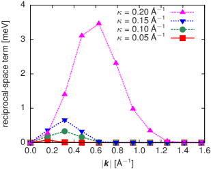
Figure 2: $k$-dependence of the reciprocal-space term $\widetilde{E}_{\bm{k}}(k)$ for different Ewald splitting parameters $\kappa$. The $k\rightarrow 0$ behavior of $\widetilde{E}_{\bm{k}}(k)$ is governed by $Q(k)$, which results in negligible contributions of the small $k$-values to the total energy.

Finally the sum in Eq. (24) is evaluated for the given $k$-mesh with truncation sphere in the reciprocal-space. The difference between this approach of a spherical truncation and the full summation is very small because of the exponential damping in Eq. (27), as seen in the rapid decay of $\widetilde{E}_{\bm{k}}(k)$ for increasing $k$ in Fig. 2. In Fig. 3 the $\kappa$-dependence of the reciprocal-space term $\widetilde{E}^{\text{tot}}_{\bm{k}}$ is illustrated in a logarithmic plot. For the chosen damping of $\kappa=0.1\,\text{\AA}^{-1}$ we get

$$\frac{1}{N}\widetilde{E}^{\text{tot}}_{\bm{k}}=3.3\,\mu{\text{e}V},$$ (28)

which is small compared to the real-space part and can thus be neglected.

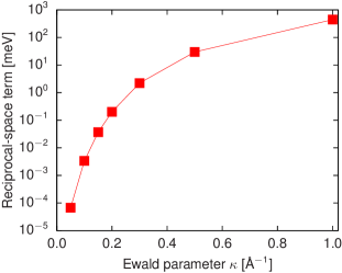
Figure 3: Logarithmic plot of the reciprocal-space term $\widetilde{E}^{\text{tot}}_{\bm{k}}$ for different Ewald splitting parameters $\kappa$. For sufficiently small $\kappa$, there is no noticeable contribution to the total energy compared to the real-space part.

IV Results

The damped and smoothly cut off TS potential was used to study the same thermodynamic and structural properties the original authorsTangney and Scandolo (2002) examined for the Ewald-summed potential.

IV.1 Equation of State and Bonding Properties

We compare the equation of state of liquid silica at 3100 K to experimentsGaetani et al. (1998), ab initio results and, of course, the full TS potential in Fig. 4. Pressures were obtained as averages along constant-volume MD runs of approximately 10 ps following 10 ps of equilibration and with simulation cells containing 4896 atoms. We reproduced the good agreement of the full TS potential with the experimental results; both the full TS potential and our damped and smoothly cut off TS potential match even better with experiment than the ab initio results. As already mentioned by the original authorsTangney and Scandolo (2002) the BKS model systematically underestimates the volume by $\approx$ 13%. The large scatter of the ab initio results can be explained with the system size and time constraints of this method: especially for low pressures, the system cannot be equilibrated completely.

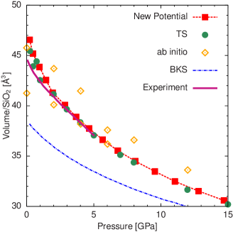
Figure 4: Equation of state of liquid silica for damped and smoothly cut off TS potential compared to experimentGaetani et al. (1998), ab initio simulations and classical simulations with BKS and the full TS potentialTangney and Scandolo (2002).

On a microscopic level, the Si–O–Si angle distribution was determined from multiple MD simulation runs at 3100 K and various pressures. The results are shown in Fig. 5, and are in agreement with the full TS potential and ab initio results.

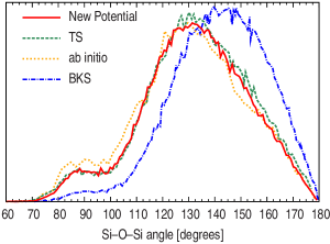
Figure 5: Oxygen centered angle distribution in liquid silica for the new potential compared to simulations with BKS and the full TS potential as well as ab initio calculations.Tangney and Scandolo (2002)

In Fig. 6 the percentage of $N$-fold coordinated silicon atoms in liquid silica at 3100 K as a function of pressure is illustrated. Our results are compared to simulations with the full TS potential,Tangney and Scandolo (2002) which agree rather well with ab initioBarrat et al. (1997) results.

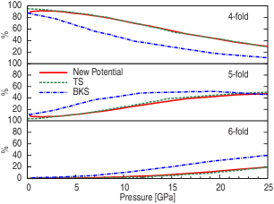
Figure 6: Percentage of $N$-fold coordinated silicon atoms in liquid silica at 3100 K as a function of pressure compared to simulations with BKS and the full TS potentialTangney and Scandolo (2002).

To sum up, the equation of state and the bonding properties of liquid silica, which the original authorsTangney and Scandolo (2002) examined for the Ewald-summed potential, can be reproduced very well by using the damped and smoothly cut off TS potential, while using dramatically less CPU time. Due to the linear scaling of computational effort in the system size, this advantage becomes even more pronounced the larger the system is.

IV.2 Crystal Structure Data

We also probed the damped and smoothly cut off TS potential by simulating the most important low pressure crystal structures quartz, cristobalite and coesite. The relevant equilibrium variables density, Si–O–Si angle and the lattice parameters at 300 K are given in Tables 1,  2 and 3. The average relative deviation of the data from the experimental results is $\approx$ 0.9%, which is a comparatively good agreement. By contrast, the BKS potential differs by $\approx$ 2.1% on average. Note that simulations with the full TS potential yield a relative deviation of the parameters that averages at merely $\approx$ 0.7%. This decrease in precision might be countered by redetermining the parameters for the smoothed and damped TS force field, as we suggest in Sec. V. Additionally, the ordered crystals might be more susceptible to spontaneous polarization compared to the liquid, however we could not confirm this in our simulations.

It should be noted, however, that the TS potential was optimized to reproduce atomistic properties of liquid SiO₂ at 3000 K. For this reason, its application to low-temperature crystalline systems should be closely monitored. In the case of cristobalite we found that both the full TS potential and the smoothly truncated potential energetically favor a slightly different orientational arrangement of the fundamental SiO₄ tetrahedra at low temperatures, with only little consequence on quantities given in Tab. 2.

Table 1: Quartz

	Expt.	New Potential	TS	BKS2
$a$ (Å)	$4.916$	$4.872$	$4.925$	$4.941$
$c$ (Å)	$5.405$	$5.359$	$5.386$	$5.449$
$\rho$ (g/cm3)	$2.646$	$2.718$	$2.665$	$2.598$
Si–O–Si (∘)	$143.7$	$142.1$	$144.5$	$148.1$

Table 2: Cristobalite

	Expt.	New Potential	TS	BKS4
$a$ (Å)	$4.969$	$5.015$	$4.936$	$4.920$
$c$ (Å)	$6.925$	$6.999$	$6.847$	$6.602$
$\rho$ (g/cm3)	$2.334$	$2.268$	$2.412$	$2.515$
Si–O–Si (∘)	$146.4$	$147.1$	$144.0$	$143.9$

Table 3: Coesite

	Expt.	New Potential	TS	BKS6
$a$ (Å)	$7.136$	$7.123$	$~{}7.165{}$	$~{}7.138{}$
$b$ (Å)	$7.174$	$7.161$	$7.162$	$7.271$
$c$ (Å)	$12.369$	$12.347$	$12.377$	$12.493$
$\beta$ (∘)	$120.34$	$120.34$	$120.31$	$120.76$
$\rho$ (g/cm3)	$2.921$	$2.940$	$2.933$	$2.864$
Si–O–Si (∘)	$143.6$	$144.2$	$144.0$	$150.5$

V Conclusion

In this work, we have demonstrated that the advantages of the TS polarizable force field can be captured and reproduced in MD simulations with a strictly finite interaction range. To this end, we have shown that the Wolf summation technique, i.e. smoothly cutting off the damped long range real space part of the electrostatic interaction, and neglecting the reciprocal space part altogether, is justified for the TS dipolar force field for silica. With a suitably large real space cut-off, the errors in the forces and energies are acceptable for the systems of interest. This can also be seen in simulation results: Our Wolf-summed TS potential can reproduce the experimental and ab initio structural properties of silica reasonably well compared to the full TS interaction.

By omitting the reciprocal space contribution, simulations with our potential can be performed with a standard finite-range MD code like IMD. Thus, it can profit from the linear scaling of computational effort with system size common to this method. Similarly, the calculations can easily and efficiently be parallelized, opening the door to large-scale calculations impossible with the standard Ewald summation technique. Moreover, once the reciprocal space part can be neglected, there is no longer any need for periodic boundary conditions. It has been shown that Wolf summation performs very well also for open or mixed boundary conditions,Wolf et al. (1999) opening up a wealth of new possibilities.

As a rule of thumb, the real space cut-off radius required for Wolf summation has been estimated as about five times the largest nearest neighbor distance of opposite charges in the system.Demontis et al. (2001) For silica, this amounts to a moderate value of about 8 Å. But even with a more conservative choice of 10 Å, for more accurate simulations, for a system with 4896 atoms we obtained a speedup of more than two orders of magnitude compared to the original code of Tangney and Scandolo. Also this performance increase makes the new method very interesting, and opens up new possibilities.

The original TS potential parameters were optimized for the full Ewald treatment of long-range interactions. Redetermining the parameters for the smoothed and damped TS force field with the actual cutoff used in simulation might improve the potential further. Additionally, using a more flexible short-range interaction than the Morse-Stretch potential suggested by Tangney and Scandolo could lead to even better results. We plan to implement the TS polarizable oxide potential model in our Force Matching code potfitBrommer and Gähler (2007) to perform this optimisation. This implementation could then be used to determine polarizable oxide potential parameters also for other materials like alumina or magnesia.