Excitation of slow MJO-like Kelvin waves in the equatorial atmosphere by Yanai wave-group via WISHE-induced convection

Abstract

The intraseasonal Madden-Julian oscillation (MJO) involves a slow eastward-propagating signal in the tropical atmosphere which significantly influences climate yet is not well understood despite significant theoretical and observational progress.

We study the atmosphere’s response to nonlinear “Wind Induced Surface Heat Exchange” (WISHE) forcing in the tropics using a simple shallow water atmospheric model. The model produces an interestingly rich interannual behavior including a slow, eastward propagating equatorial westerly multiscale signal, not consistent with any free linear waves, and with MJO-like characteristics. It is shown that the slow signal is due to a Kelvin wave forced by WISHE due to the meridional wind induced by a Yanai wave group. The forced Kelvin wave has a velocity similar to the group velocity of the Yanai waves, allowing the two to interact nonlinearly via the WISHE term while slowly propagating eastward. These results may have implications for observed tropical WISHE-related atmospheric intraseasonal phenomena.

SOLODOCH ET AL Yanai-forced MJO-like signal Aviv Solodoch, Weizmann Institute of Science, Rehovot, 76100, Israel William Boos, Zhiming Kuang, Eli Tziperman, Dept of Earth and Planetary Sciences and School of Engineering and Applied Sciences, Harvard University, 20 Oxford St, Cambridge, MA 02138-2902. wrboos@fas.harvard.edu, kuang@fas.harvard.edu, eli@eps.harvard.edu.

1 Introduction

The “Madden Julian Oscillation” (MJO) (Madden and Julian, 1971, 1994; Zhang, 2005) is the most significant intraseasonal phenomena in the tropical atmosphere. It couples convection and large-scale circulation, and propagates eastward at about 5 ms^-1, through the Indian and East to Central Pacific oceans. This is a surprisingly slow propagation when compared with a typical moist Kelvin wave speed (15-20 ms^-1).

One of the mechanisms suggested to explain the MJO was wind induced surface heat exchange (WISHE) (Emanuel, 1987; Neelin et al., 1987), according to which air-sea latent heat fluxes enhanced by surface winds are of paramount importance for forcing and organizing tropical convection. Emanuel (1987) and Neelin et al. (1987) found Kelvin-like solutions due to the convection-wind coupling in linear WISHE models. While these early solutions seem to differ significantly from observed MJO characteristics (e.g. Zhang, 2005), recent observational and model evidence suggests an important role for WISHE in MJO dynamics (Maloney and Sobel, 2004; Sobel et al., 2008). In addition, nonlinear WISHE effects seem to be important in simulated MJO-like disturbances (Raymond, 2001; Maloney and Sobel, 2004).

In light of these findings we investigate an equivalent-barotropic shallow water atmospheric model with a simple nonlinear WISHE formulation, on a beta plane. The numerical experiments yield intriguing dynamics, including a slow eastward propagating signal that shares some of the observed MJO characteristics, and its mechanism is analyzed below and also presented in the thesis of Solodoch (2010) (hereafter S2010). Given the simplicity of the model, it is not possible to conclusively demonstrate that this mechanism is applicable to the observed MJO, but we feel it is nevertheless a most interesting and nontrivial mechanism which can enrich our understanding of tropical dynamics.

2 The model

The model equations are the shallow water equations with a WISHE heating forcing term $(Q)$ (Gill, 1980),

$$u_{t}-\beta yv = -\eta_{x}+\nu\nabla^{2}u,$$ (1)

$$v_{t}+\beta yu = -\eta_{y}+\nu\nabla^{2}v,$$ (2)

$$\eta_{t}+H(u_{x}+v_{y}) = -Q(u,v,\eta)-\frac{1}{\tau}\eta.$$ (3)

$$Q = \max\left(0,A\left|\mathbf{u}+\mathbf{U}\right|(\eta-\eta_{sat})\right)$$ (4)

where $u$ and $v$ are the zonal and meridional perturbation velocities, $\eta$ is the perturbation (hydrostatic) pressure, $\nu$ the eddy diffusivity coefficient, and $\tau$ a Newtonian cooling time scale. In the standard experiment, mean surface easterlies, $\mathbf{U}=U\hat{x}$, which tend to prevail in much of the equatorial Pacific are added to the model velocity in the WISHE term only, with $U=-2$ m/s. We also set $\tau=5$ days, $\eta_{sat}=-5$ mbar and $A=2\cdot 10^{-6}$ m^-1. The equivalent depth is set to $H=50$ m, consistent with observed convectively coupled waves in the tropics having $H=10-60$ m (Wheeler and Kiladis, 1999). The typical tropical balance between convective heating and adiabatic cooling is thus implicit in (1)-(3) through this choice of $H$, and $Q$ represents only the positive-definite convective heating caused by surface heat flux variations. The model is periodic in the east-west coordinate ($x$), extends from 60S to 60N and 25,600 km in the east-west direction, and is based on the MIT GCM (Marshall et al., 1997a, b).

3 Results: slow eastward propagation of equatorial westerlies

A Hovmoller diagram of the zonal velocity $u$ at the equator, for days 80-160 after the initialization, is shown in Fig. 1a. The most prominent feature is an eastward propagating disturbance, significantly slower than the equatorial Kelvin wave (22 m/s in this model). The slow signal is an irregular, a wide band, multiscale phenomenon in space and time, and the propagation speed varies between 8-12 m/s. One wonders, of course, if this slow eastward propagating equatorial disturbance is of any relevance to the MJO, but understanding its dynamics seems a worthwhile goal in any case.

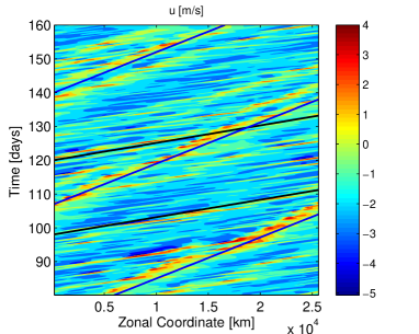
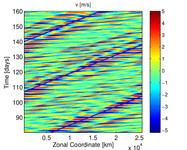
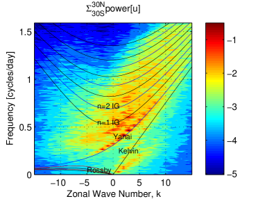
Figure 1: Hovmoller diagrams at the equator from exp 1. Top: zonal velocity, $u$ [m/s], with lines showing propagation speeds of 22 m/s and 9.5 m/s. Middle: meridional velocity, $v$ [m/s]. Bottom: Spectral power of $u(x,y,t)$, in log scale, calculated by Fourier transforming in $(x,t)$ at each latitude, and then summing the power between $\pm 30$ degrees latitude. Zonal wave number is for an equatorial circumference of 25,600 km.

Interestingly, the anomalous zonal wind is not symmetric, and a histogram analysis (not shown) shows that easterly anomalies are usually weaker than the westerly anomalies. This is reminiscent of “Westerly wind bursts” observations over the tropical oceans (Harrison and Vecchi, 1997) associated in some cases with MJO events.

A Hovmoller diagram of the equatorial meridional velocity, $v$, (Fig. 1b) shows an eastward propagating wave group, propagating with the same speed as the slow signal seen in the $u$ Hovmoller diagram. The $v$ wave group envelope is highly coherent with the slowly eastward propagating $u$ signal, while showing complex patterns of phase propagation within the eastward propagating envelope. The $v$ Hovmoller and the spectrum shown in Fig. 1c show that the $v$ signal corresponds to a group of Yanai waves propagating with the slow signal. It will be shown below that the speed of propagation of the slow signal is indeed compatible with the group velocity of long Yanai waves, and the interaction between the $u$ and $v$ fields will be explained.

Dispersion curves of equatorial waves are superimposed over the contours of the power spectrum in Fig. 1c, and most of the spectral power is seen to be concentrated near these dispersion curves. The linear wave modes with the most power are the Yanai wave and the Inertia-Gravity $n=1$ wave, and the Kelvin wave is also excited.

However, significant power is concentrated in a feature not associated with any linear wave mode, which is located in $k-\omega$ space beneath the dispersion curve of the Kelvin wave. This feature corresponds to the slowly propagating signal seen in the Hovmoller diagrams. A cross section along the slowly propagating signal (Fig. 2, blue line) shows its variance to be symmetric in latitude with a Gaussian structure centered around the equator, similarly to a Kelvin wave. It also lies close to a linear line in $k-\omega$ space, and appears in the $\eta$ field, yet is virtually non-existent in the $v$ power spectrum (S2010). These are all characteristics of a Kelvin wave, except that this feature has the “wrong” meridional scale when compared to the Gaussian Kelvin structure given the model’s equivalent depth (Fig. 2) and this is further explained below. We also note that most of the energy of the “sub-Kelvin” signal is in the $k=1$ planetary scale, and the energy decreases with $k$. The sub-Kelvin variability explains 50% of the zonal wind variability at the equator. The above description makes it clear that the slow eastward propagating signal clearly combines both low frequency Kelvin-like waves, and higher frequency Yanai waves.

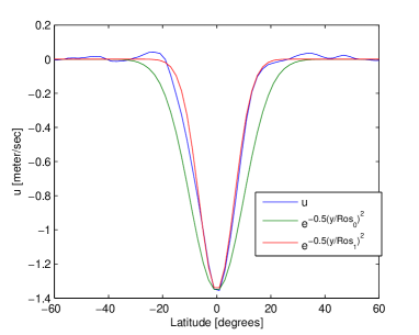
Figure 2: The meridional structure of the slowly propagating signal. The blue line shows a meridional cross section showing the root time-mean square of zonal velocity anomalies at the middle meridian of the domain. Green: a Gaussian meridional structure of the Kelvin or $v$ velocity of the Yanai wave. Red: a Gaussian fit based on a Rossby radius of deformation smaller by a factor of $\sqrt{2}$ than the model value.

4 The mechanism

We now show that the slow eastward propagating signal is a forced Kelvin wave, excited by the envelope of a Yanai wave-group. The efficient excitation is possible due to two factors. First, the forced Kelvin velocity is very similar to the Yanai group velocity. Second, the meridional structure of the slow Kelvin waves signal is identical to that of the square of the Yanai wave, which allows the Kelvin wave to be excited through the nonlinear WISHE heating term.

Starting from the heating forcing term, note that the power series expansion of the WISHE term $Q$ is,

$$(\eta+|\eta^{*}|)\sqrt{(u+U)^{2}+v^{2}}=|\eta^{*}||U|+\eta|U|-|\eta^{*}|u$$

$$- \eta u+\frac{|\eta^{*}|}{2|U|}v^{2}+\frac{1}{2|U|}{\eta}v^{2}+\frac{|\eta^{*}|}{2|U|^{2}}uv^{2}+...$$

Although the formal convergence criterion for this power series is not always satisfied in the model, a correlation analysis of the different terms in this expansion with the full heating $Q$ shows that the $v^{2}$ term accounts for much of the heating variability. $v$ itself is, in turn, dominated by the contribution due to the Yanai waves. Now, we are interested in the slow forcing of a Kelvin wave by the meridional velocity due to the Yanai waves, $v_{Yanai}$, leading us to examine the time average of $(v_{Yanai})^{2}$. This represents the energy of the Yanai waves which therefore moves at the Yanai group velocity $c_{g}(k)$ and may be written as ${\langle}v_{Yanai}^{2}\rangle=\sum_{k}\frac{1}{2}\left((\widehat{v_{Y}^{2}})_{k}e^{ik(x-c_{g}t)}+c.c.\right)$, where c.c. is complex conjugate, and $(\widehat{v_{Y}^{2}})_{k}$ is the amplitude of the envelope of $v^{2}$ due to the Yanai waves at wavenumber $k$.

An important insight here is that the Yanai $v$ field has a Gaussian structure, $\Psi_{0}=\exp({-{y^{2}}/({2R_{0}^{2}})})$, so that its square results in WISHE forcing of the form $Q{\sim}v^{2}\sim\exp({-2{y^{2}}/({2R_{0}^{2}})})=\exp({-{y^{2}}/({2R_{1}^{2}})})$, where $R_{1}=R_{0}/{\sqrt{2}}$. This also implies an equivalent depth of the forced signal of $H/4$ where $H$ is the model’s specified equivalent depth. In other words, the square of the Yanai wave $v$ velocity has the Gaussian structure corresponding to a smaller equivalent depth, forcing a Kelvin wave like response with a similarly smaller effective equivalent depth. This implies that this forced Kelvin wave propagates slower than the free Kelvin waves in the system, leading to the observed slowly propagating signal.

We found in the numerical simulation above that $Q$ excites a Kelvin-like signal with a very small $v$ velocity. Consider therefore the following set of equations for a forced Kelvin wave by setting $v=0$ and ignoring dissipation,

$$u_{t} = -\eta_{x},$$ (5)

$$\beta yu = -\eta_{y},$$ (6)

$$\eta_{t}+Hu_{x} = -G(\widehat{v_{Y}^{2}})_{k}e^{-2\frac{y^{2}}{2R^{2}}}e^{ik(x-c_{g}t)}.$$ (7)

Assuming $G(\widehat{v_{Y}^{2}})_{k}$ to be a constant amplitude of the forcing at wavenumber $k$ (see discussion below), the forced Kelvin solution would be a superposition of the solutions with the same functional form as the forcing,

$$(u,\eta)=e^{-\frac{y^{2}}{2R_{1}^{2}}}e^{ik(x-c_{g}t)}(u_{0},\eta_{0}).$$ (8)

Inserting (8) into (5-6) leads to the condition $c_{g}={\beta}R_{1}^{2}={c_{0}}/{2}$ where $c_{0}$ is the free Kelvin wave speed in the model. Interestingly, this condition is satisfied exactly for a Yanai wave of $k=0$ as can be verified from the Yanai dispersion relation, and more generally is approximately satisfied for long Yanai waves of $-5{\leq}k\leq 10$. This interesting coincidence allows the slowly propagating solution (8) to be excited by the Yanai waves. Inserting this relation into (7) yields the forced wave solution,

$$u_{0}=\frac{iG(\hat{v_{Y}^{2}})_{k}}{k(c_{0}^{2}-c_{g}^{2})},\quad\eta_{0}=c_{g}u_{0},\quad v=0.$$ (9)

These expressions are found to be consistent to a very good approximation with the numerical simulation. The disturbance clearly has the strongest response at the longest wavenumbers ($k=1$), as is actually found for the sub-Kelvin spectrum in our simulation (and, interestingly, also for the observed MJO). Fig. 2 shows a meridional cross section through the slowly propagating signal (blue), demonstrating that its structure is indeed very nearly a Gaussian (red) corresponding to the square of the Yanai wave structure (green). This provides an explicit and strong evidence of the nonlinear forcing mechanism described above.

Observations show that the MJO convection is mostly co-located with its surface westerlies in the west-Pacific and with surface convergence in the Indian ocean (Zhang, 2005). The Hovmoller plot of $u$ and $v$ (Fig. 1a,b) show that the maximum of the Yanai envelope (and thereby its contribution to WISHE) is nearly co-located with the maximum of the sub-Kelvin signal at all times. Similarly, the snapshot of Fig. 3 shows the maximum Yanai induced $v^{2}$ WISHE envelope to be co-located with, or slightly lead, the maximum sub-Kelvin westerlies, similar to the corresponding relationship between MJO convection and circulation, as observed.

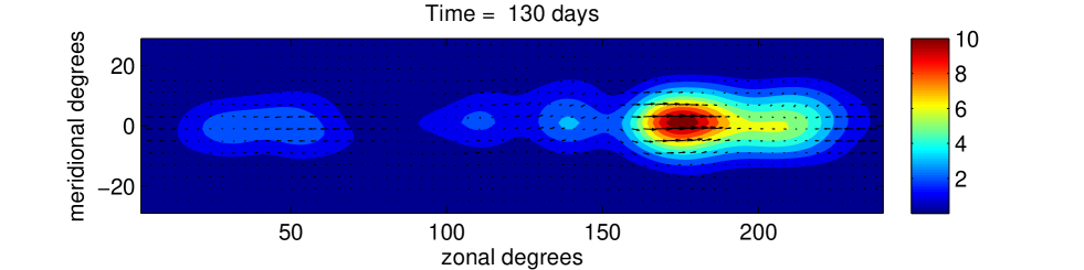
Figure 3: Demonstrating the longitudinal phase between the heating and the slow signal wind response. Arrows: winds corresponding to the slowly propagating signal (obtained by filtering the full solution in $k,\omega$ space, keeping only the area under the kelvin wave dispersion curve corresponding to the show signal alone. Contours: the 2-day running time-averaged Yanai wave contribution to the heating ${\langle}v_{Yanai}^{2}{\rangle}$.

The Yanai waves which force the slow signal may themselves be destabilized by the WISHE term in the presence of easterly winds (Emanuel, 1993). However, the Yanai fields on the left hand side of the continuity equation (3) ($\eta$, $u_{x}$, $v_{y}$) are antisymmetric in $y$ ($e^{-\frac{1}{2}({y}/{R})^{2}}2{y}/{R}$) and therefore cannot be forced by the symmetric, Gaussian, Kelvin wave fields ($u$ and $\eta$) even when raised to some power, justifying the above approximation of $G(\widehat{v_{Y}^{2}})_{k}$ as a constant amplitude of the forcing not affected by the Kelvin waves.

5 Sensitivity study

The main features of the slowly propagating signal are found to be robust with respect to different meridional boundary condition, initial conditions, and the value of the mean parametrized zonal velocity, $U$ (as long as it is easterly). The signal also appears if the WISHE forcing term is limited to the equatorial domain only, as long as this forcing domain is not smaller than about 6 degrees latitude. The slow signal is also quite robust to the values of model parameters, yet does not appear, of course, for large values of the dissipation parameters or too small values of the WISHE coefficient. Given that the WISHE coefficient, $A$, idealizes the product of a transfer coefficient and several other poorly constrained thermodynamic factors in a bulk transfer formula (Emanuel, 1987; Neelin et al., 1987, e.g.,), it is not obvious whether the value used here is realistic. Additional sensitivity experiments and analysis is given in S2010.

6 Conclusions

An equivalent-barotropic shallow water model driven by nonlinear WISHE convective heating was used to study tropical atmosphere intraseasonal phenomena. A slowly eastward propagating signal appears robustly in the experiments, with about half the speed of a linear Kelvin wave. The slowly eastward propagating equatorial signal is interesting because it shares some major characteristics with the large scale fields of the MJO, some of which are not explained by current theories.

The slow eastward propagating signal was shown to be a forced Kelvin wave with a meridional spatial structure consistent with an equivalent depth smaller than that specified in the model. The signal is also coherent with a group of long Yanai waves which has a group velocity similar to that of the slow forced Kelvin wave. We showed that the Yanai group nonlinearly forces the slow Kelvin-like signal through the WISHE term, and explained how the nonlinear WISHE term leads to the smaller effective equivalent depth and slow propagation of the signal. The suggested mechanism predicts the slower Kelvin wave meridional structure and speed, as well as the right order of magnitude of the amplitude. The excited signal in the numerical simulations is strongest at $k=1$ and 2, again consistent with the suggested mechanism. The phenomenon has a multiscale character in space and time, and an interesting and novel aspect of the mechanism proposed here is the critical role of higher frequency motions involving the Yanai waves. Concurrently with Solodoch [2010] and the present study, a somewhat related idea has recently been presented in a conference abstract (Yang and Ingersoll, 2009).

The slow signal is reminiscent of some of the main features of the MJO, in particular its wide-band nature, slow eastward propagation, its Kelvin-like large scale structure at and east of its convection center, and its spectral power peaks at the $k=1$ and $2$ wavenumbers. Additionally, there is asymmetry in zonal wind toward higher westerlies than easterlies, particularly close to the convection center.

Preliminary results to be reported elsewhere (Solodoch et al., 2010) show that the mechanism found here is also relevant to more detailed models, with significantly more realistic convective parameterizations. Although it is clearly premature to propose that the mechanism found here is applicable to the MJO, exploring the suggested mechanism in more realistic models and in observations may prove fruitful.

References

- Emanuel (1987) Emanuel, K. A. (1987), An air-sea interaction model of intraseasonal oscillations in the tropics, J. Atmos. Sci., 44, 2324–2340.
- Emanuel (1993) Emanuel, K. A. (1993), The effect of convective response time on WISHE modes, J. Atmos. Sci., 50, 1763–1775.
- Gill (1980) Gill, A. E. (1980), Some simple solutions for heat-induced tropical circulation, Q. J. R. Meteorol. Soc., 106, 447–462.
- Harrison and Vecchi (1997) Harrison, D. E., and G. A. Vecchi (1997), Westerly wind events in the tropical Pacific, 1986-95, J. Climate, 10(12), 3131–3156.
- Madden and Julian (1971) Madden, R. A., and P. R. Julian (1971), Detection of a 40-50 day oscillation in zonal wind in tropical Pacific, J. Atmos. Sci., 28(5), 702–&.
- Madden and Julian (1994) Madden, R. A., and P. R. Julian (1994), Observations of the 40-50-day tropical oscillation- a review, Mon. Weath. Rev., 122, 814–837.
- Maloney and Sobel (2004) Maloney, E. D., and A. H. Sobel (2004), Surface fluxes and ocean coupling in the tropical intraseasonal oscillation, J. Climate, 17, 4368 4386.
- Marshall et al. (1997a) Marshall, J., A. Adcroft, C. Hill, L. Perelman, and C. Heisey (1997a), A finite-volume, incompressible navier stokes model for studies of the ocean on parallel computers, J. Geophys. Res., 102, C3, 5,753–5,766, mars-eta:97b.
- Marshall et al. (1997b) Marshall, J., C. Hill, L. Perelman, and A. Adcroft (1997b), Hydrostatic, quasi-hydrostatic and nonhydrostatic ocean modeling, J. Geophys. Res., 102, C3, 5,733–5,752, mars-eta:97a.
- Neelin et al. (1987) Neelin, J. D., I. M. Held, and K. H. Cook (1987), Evaporation-wind feedback and low-frequency variability in the tropical atmosphere, J. Atmos. Sci., 44, 2341–2348.
- Raymond (2001) Raymond, D. J. (2001), A new model of the Madden-Julian oscillation, J. Atmos. Sci., 58(18), 2807–2819.
- Sobel et al. (2008) Sobel, A. H., E. D. Maloney, G. Bellon, and D. Frierson (2008), The role of surface heat fluxes in tropical intraseasonal oscillations, Nature Geosicence, 1, 653–657.
- Solodoch (2010) Solodoch, A. (2010), Excitation of slow kelvin waves in the equatorial atmosphere by yanai wave-group-induced convection, Master’s thesis, Weizmann Institute of Science.
- Solodoch et al. (2010) Solodoch, A., W. Boos, Z. Kuang, and E. Tziperman (2010), Mjo-like signal in due to yanai-wave forcing in intermediate-complexity atmospheric models, in prep.
- Wheeler and Kiladis (1999) Wheeler, M., and G. N. Kiladis (1999), Convectively coupled equatorial waves: Analysis of clouds and temperature in the wavenumber-frequency domain, J. Atmos. Sci., 56(3), 374–399.
- Yang and Ingersoll (2009) Yang, D., and A. P. Ingersoll (2009), Testing a rossby-wave theory of the mjo, in AGU fall meeting abstract.
- Zhang (2005) Zhang, C. D. (2005), Madden-julian oscillation, Rev. Geophys., 43.