Hidden Quantum Markov Models and non-adaptive read-out of many-body states

Abstract

Stochastic finite-state generators are compressed descriptions of infinite time series. Alternatively, compressed descriptions are given by quantum finite-state generators [K. Wiesner and J. P. Crutchfield, Physica D 237, 1173 (2008)]. These are based on repeated von Neumann measurements on a quantum dynamical system. Here we generalise the quantum finite-state generators by replacing the von Neumann projections by stochastic quantum operations. In this way we assure that any time series with a stochastic compressed description has a compressed quantum description. Moreover, we establish a link between our stochastic generators and the sequential readout of many-body states with translationally-invariant matrix product state representations. As an example, we consider the non-adaptive read-out of 1D cluster states. This is shown to be equivalent to a Hidden Quantum Model with two internal states, providing insight on the inherent complexity of the process. Finally, it is proven by example that the quantum description can have a higher degree of compression than the classical stochastic one.

1 Introduction

The physical laws underlying quantum computation are a mixed blessing. On the one hand, a growing body of theoretical results suggests that a computational device whose components are directly governed by quantum physics may be considerably more powerful than its classical counterpart. As proof, several quantum algorithms have been constructed. The most celebrated ones are the factoring algorithm by Shor [1], suggesting an exponential speed-up over classical algorithms, and the data-base search algorithm by Grover [2], proving a linear speed-up. They are quantum versions of algorithms that improve the efficiency of algorithms usually implemented on classical Turing machines.

Contrary to this progress on the theoretical side, building a quantum computer in practice faces many hurdles. Implementations of quantum Turing machines must maintain high degrees of internal coherence and insulation to outer disturbances during operation. Thus, the current implementations remain with highly finite systems, much more of the character of finite-state machines than Turing machines [3]. In the yet to be completed hierarchy of quantum computational architectures quantum Turing machines are decidedly more powerful than finite-state machines. However, because of the “finiteness” of current implementations of quantum algorithms the lower part of this hierarchy and its potential computational power are of great interest.

At this point, a look at information creation in dynamical systems turns out to be useful. Recently, one of the authors introduced a synthesis of quantum dynamics, information creation, and computing [4, 5]. This lead to methods useful for analysing how quantum processes store and manipulate information. A quantum process was defined as a probability distribution over measurement outcomes of a repeatedly measured quantum system, formally represented as a process language. A measurement-based quantum-computation hierarchy was developed, providing insights into the information processing in quantum dynamical systems. This computational hierarchy allows for a classification of quantum dynamical systems in terms of the process languages they generate. Following this ansatz, we concentrate here on a characterisation of generators of process languages. The characterisation of recognisers is analogous (up to some exceptions [4]) but will not be addressed here.

The quantum finite-state machines introduced by Wiesner and Crutchfield in 2008 [4] generate bit sequences by applying a projective (von Neumann) measurement repeatedly to an otherwise dynamically evolving quantum system. In the following, we therefore refer to them as quantum von Neumann finite-state generators. However, there are regular languages which cannot be generated by a von Neumann finite-state machine [4]. An example is an alternating binary sequence with different probabilities for the two binary symbols [4]. Here we point out that it is possible to overcome this problem by replacing the projective measurements of von Neumann finite-state machines by stochastic quantum operations, i.e., generalized measurements described in the quantum operation formalism. We call the resulting stochastic processes Hidden Quantum Markov Models (HQMM).

Quantum operations are the most general transformations that a quantum state can undergo. This includes the possibility of the state being (partially) measured and the possibility of resetting or transforming the system conditional on the measurement outcome [6]. Contrary to projective measurements, the state of the system after a measurement may depend not only on the respective measurement outcome. In general, it may retain information about the state of the system prior to the operation and hence also information about previous measurement outcomes. Thus, the system acquires a memory which may be anything from classical to quantum. As a consequence, any process language which can be generated by a classical stochastic finite-state machine can now be generated by a quantum finite-state machine. Secondly, any iterative quantum process can now be represented as a quantum finite-state machine. Finally, we show by example that there are process languages which are generated with fewer resources using quantum finite-state machines compared to classical ones.

There are six sections in this paper. Section 2 reviews stochastic processes, their formal representation as process languages, and stochastic finite-state machines as generators of such process languages. This is followed by a review of quantum processes and von Neumann finite-state generators in Section 3. Section 4 introduces HQMMs as computation-theoretic representations of general finite-dimensional quantum operations and presents an information-theoretic analysis of quantum systems under generalised measurements. Section 5 shows that the non-adaptive read-out of a 1D cluster state generates the same process languages as a repeatedly measured dynamical open quantum two-level system. It therefore constitutes an example of a HQMM. Finally, we summarize our results and draw attention to some open questions in Section 7.

2 Stochastic Processes

Consider the temporal evolution of some natural system. The evolution is monitored by a series of measurements—numbers sequentially registered. Considering the numbers to be discrete, each such measurement can be taken as a discrete random variable $X_{i}$. The probability distribution $\mathrm{Pr}(X_{-\infty}^{+\infty})$ over bi-infinite sequences $X_{-\infty}^{+\infty}$ of these random variables is what we refer to as a stochastic process. Such a process is a complete description of a system’s behaviour. An important question for understanding the structure of natural systems therefore is what kinds of stochastic processes there are. This question can be studied using stochastic finite-state generators which are a classification tool for stochastic processes.

The distribution over sequences of random variables as a representation of a stochastic process is merely an enumeration of probabilities. It is not a very practical representation, let alone does it allow for any insights. Thus, it is desirable to find a more compact representation of a process than just the probability distribution over sequences.

Among all possible stochastic processes, several models have proven successful in order to model a wide range of practical situations. One such class of processes are the so-called Hidden Markov Models (HMM from now on). There are several possible ways to define a HMM. The most common among mathematicians is as a stochastic process S for which every symbol $s_{n}$ is generated conditionally from a Markovian process X, with probability $\mathrm{Pr}(s_{n}|x_{n})$. The Markov process X goes unobserved. This definition is called the Moore HMM. An equivalent definition, more common in the computer science literature is that of a Mealy HMM, which can be formulated as the process generated by a stochastic finite-state generator, and will be the one considered in the present work. Stochastic finite-state generators differ from finite-state machines used for recognition of regular languages in two ways. They have probabilistic transitions, similar to Paz’s probabilistic automata [7]. And they generate sequences instead of recognising them. In the following, we use the minimal number of internal states that a device needs in order to generate a stochastic language as a measure of complexity [8, 9]. This quantification of complexity is complimentary to the notion of algorithmic complexity [10, 11].

2.1 Stochastic finite-state generators and hidden Markov models

Let us recall the definition of a stochastic finite-state generator from Ref. [4]. A stochastic finite-state generator is a tuple $(S,\mathcal{A},{\bf T})$ where $S$ is a finite set of states, $\mathcal{A}=\{s\}$ is a countable set of symbols, output alphabet, and ${\bf T}=\{T_{s}:s\in\mathcal{A}\}$ are square substochastic matrices of dimension $|S|$, such that $\sum_{s}T_{s}$ is stochastic. The system undergoes transitions between internal states and every transition has an associated output symbol. The generator is fully characterized when all conditional probabilities $\mathrm{Pr}(s;j|j_{0})$ are given, that is, the probability of yielding symbol $s\in\mathcal{A}$ and going to state $j$ conditional on the machine being in state $j_{0}$. These probabilities are summarized by the set of substochastic matrices $T_{s}$, where $[T_{s}]_{j\,j_{0}}=\mathrm{Pr}(s;j|j_{0})$ . The sum $\sum_{s\in\mathcal{A}}T_{s}$ is a stochastic matrix which describes the Markovian evolution of the state space when the output symbols are disregarded. These automata can be represented by a directed graph where nodes correspond to states and directed edges correspond to transitions with non-zero probability (see Ref. [4] for details and Fig. 1 for an example of such a representation).

The computation of word probabilities is easily done in terms of the matrices $T_{s}$. The conditional probability of word $\textbf{s}=(s_{1},\ldots,s_{n})$ given an initial state $j_{0}$ is

$$\mathrm{Pr}(\textbf{s}|j_{0})=\sum_{j_{1},j_{2},\ldots j_{n}}\mathrm{Pr}(s_{n};j_{n}|j_{n-1})\cdots\mathrm{Pr}(s_{2};j_{2}|j_{1})\mathrm{Pr}(s_{1};j_{1}|j_{0})$$ (1)

which can be written as

$$\mathrm{Pr}(\textbf{s}|j_{0})=\sum_{j_{n}}\left[T_{\textbf{s}}\right]_{j_{n}\,j_{0}}~{},$$ (2)

where we have defined $T_{\textbf{s}}=T_{s_{n}}\cdots T_{s_{2}}T_{s_{1}}$. Finally, the state of the machine can be a statistical mixture of all possible internal states, which is conveniently described by a vector $|\pi\rangle$. This can be used as a prior distribution when the initial state is uncertain. The stable stochastic process is obtained from the steady state of the machine, defined as the eigenvector $|\pi^{\star}\rangle$ with eigenvalue 1 of $T=\sum_{s}T_{s}$, namely

$$|\pi^{\star}\rangle=\sum_{s\in\mathcal{A}}T_{s}|\pi^{\star}\rangle~{}.$$ (3)

Finally, word probabilities can be computed by defining the vector $|1\rangle=(1,1,\ldots,1)^{T}$,

$$\mathrm{Pr}(\textbf{s})=\langle 1|T_{s_{n}}\cdots T_{s_{2}}T_{s_{1}}|\pi^{\star}\rangle~{}.$$ (4)

Given a stochastic finite-state generator and a prior probability distribution $|\pi_{0}\rangle$ of the machine state, all word probabilities are established and a HMM is uniquely defined.

2.2 Example of a stochastic finite-state generator

As an example we give the stochastic finite-state generator for the Even-Process whose language consists of blocks of even numbers of $1$’s bounded by $0$’s. The substochastic transition matrices are

$$T_{0}=\left(\begin{array}[]{cc}\frac{1}{2}&0\\ 0&0\end{array}\right)~{}~{}\mathrm{and}~{}~{}T_{1}=\left(\begin{array}[]{ccc}0&1\\ \frac{1}{2}&0\end{array}\right)~{}.$$ (9)

Again, notice that left-multiplication is used. The corresponding graph is shown in Fig. 1. The set of irreducible forbidden words is countably infinite [12]: $\mathcal{F}=\{01^{2l+1}0:l=0,1,2,\ldots\}$. As a consequence the words in the Even-Process have a kind of infinite correlation: the “evenness” of the length of $1$-blocks is respected over arbitrarily long words. This makes the Even-Process effectively non-finite: As long as a sequence of $1$’s is produced, memory of the sequence persists [13].

Figure 1: A deterministic generator of the Even-Process: Blocks of an even number of $1$s are separated by $0$s. Only the asymptotically recurrent states are shown. Edges are labeled $p\,|\,s$, where $s\in\mathcal{A}$ and $\mathrm{Pr}(s;i|j)=[T_{s}]_{ij}$.

3 Quantum Processes

We now turn to quantum systems and the process languages they generate. As with stochastic processes, we assume that the evolution of a quantum system is recorded as a sequence of measurement outcomes. Just like before, the distribution over sequences of these random variables is a process. A computation-theoretic representation of a process generated by a quantum systems is the quantum finite-state machine introduced by one of the authors [4]. These machines, reviewed below, are based on a von Neumann measurement. In order to distinguish them from the more general Hidden Quantum Models introduced later on, we will call them in the following von Neumann finite-state generators.

3.1 Quantum von Neumann finite-state generators

Like stochastic generators, a quantum von Neumann finite-state generator, as introduced in [4], outputs a symbol $s\in\mathcal{A}$ and updates its internal state $\psi$. Now $\psi$ belongs to an $|S|$-dimensional Hilbert space $H$ instead of belonging to a set $S$, and is consistently denoted throughout the quantum information literature by $|\psi\rangle$. The classical states $j\in S$ correspond to an orthonormal basis in $H$, $\{|\psi_{j}\rangle\}$. Properly normalized linear combinations of $|\psi_{j}\rangle$ are also allowed as state vectors. Symbols are obtained by measuring the quantum system. For the von Neumann generators only von Neumann measurements are considered, which are described by a complete set ${\bf P}$ of projection operators,

$$\mathbf{P} = \{P_{s}:s\in\mathcal{A}~{}{\rm and}~{}\sum_{s}P_{s}=\mathbb{I}\}~{}\,.$$ (10)

Between measurements, a unitary transformation $U$ is applied to the system. The overall effect can be described by the operators $T_{s}=P_{s}U$. Starting with the state $|{\psi_{t}}\rangle$ at time $t$ symbol $s$ is put out and $|\psi_{t+1}(s)\rangle=P_{s}U|\psi_{t}\rangle$ is the (unnormalised) state at the next time step. In general, $|\psi(\textbf{s})\rangle$ denotes the resulting state after starting with $|\psi\rangle$ and obtaining measurement outcomes s. The unnormalized state $|\psi(\textbf{s})\rangle$ can be expressed as

$$|\psi(\textbf{s})\rangle=T_{\textbf{s}}|\psi\rangle~{},$$ (11)

where again $T_{\textbf{s}}=T_{s_{n}}\cdots T_{s_{2}}T_{s_{1}}$. The probability of obtaining the word s from state $|\psi\rangle$ is given by

$$\mathrm{Pr}(\textbf{s})=\||\psi(\textbf{s})\rangle\|^{2}=\langle\psi|T_{\textbf{s}}^{\dagger}T_{\textbf{s}}|\psi\rangle~{}.$$ (12)

3.2 Density matrix representation

The above formulation of a von Neumann finite-state generator is developed in analogy to a stochastic finite-state generator. A more convenient way, and at the same time more general, is a formulation in terms of density matrices [4, 14]. This allows to describe the most general state of the system, accounting for classical uncertainties as well as quantum indeterminacy. A state $|\psi\rangle$ is then described by density matrix $\rho=|\psi\rangle\langle\psi|$. The action of $T_{\textbf{s}}$ on $|\psi\rangle$ is replaced by

$$\mathcal{T}_{\textbf{s}}\rho=T_{\textbf{s}}|\psi\rangle\langle\psi|T_{\textbf{s}}^{\dagger}~{}.$$ (13)

Here $\mathcal{T}_{\textbf{s}}$ is a linear transformation on $\rho$, usually called a superoperator. The probability of obtaining word s then reads

$$\mathrm{Pr}(\textbf{s})=\tr[\mathcal{T}_{\textbf{s}}\rho]~{}.$$ (14)

The density operator formalism will allow for a powerful generalization of the von Neumann finite-state generator.

3.3 Example of a von Neumann finite-state generator

An example of a von Neumann finite-state generator is shown in Fig. 2. It generates the Even-Process language we are already familiar with. It consists of blocks of even numbers of $1$’s bounded by $0$’s. It’s transition matrices $T_{s}$ can be constructed from the following projection operators $P_{s}$ and the unitary matrix $U$ [4],

$$P_{0}=\left(\begin{array}[]{ccc}1&0&0\\ 0&0&0\\ 0&0&0\end{array}\right),~{}P_{1}=\left(\begin{array}[]{ccc}0&0&0\\ 0&1&0\\ 0&0&1\end{array}\right),~{}U=\left(\begin{array}[]{ccc}\frac{1}{\sqrt{2}}&0&-\frac{1}{\sqrt{2}}\\ \frac{1}{\sqrt{2}}&0&\frac{1}{\sqrt{2}}\\ 0&-1&0\end{array}\right)~{}.$$ (24)

The corresponding directed graph is shown in Fig. 2. This generator consists of 3 internal quantum states. This is the smallest dimension needed to generate the Even Process with this kind of generators.

Figure 2: von Neumann finite-state generator for the Quantum Even-Process.

3.4 More general quantum processes

Notice that the von Neumann finite-state generator above has three states which is more than the stochastic generator in Section 2.2 required. This means, the quantum representation is less compressed than the classical one. This is rather counterintuitive. As we shall see below, the reason for this is the restriction to unitary transformations $U$ and projective measurements $P_{s}$. No room is left for interaction with auxiliary quantum systems, or the resetting of parts of the system. However, physical systems with such couplings – and many quantum technology experiments relying on them – can be relatively simple. Hence realistic measurements are often imperfect and noisy, where the von Neumann measurements are an idealization. We will see that extending the formalism to density operators will allow for, not only describing more realistic processes, but also encompass the whole class of classical generators.

4 Hidden Quantum Models

In this section we define the Hidden Quantum Markov Model (HQMM), based on the notion of quantum operation. The spirit underlying our definition follows exactly the same lines as the definition of a HMM. In a HMM (HQMM) there is an underlying Markovian (Quantum) process which rules the probability of the symbols generated. We will see how word probabilities and the steady state for HQMMs are obtained in full analogy to HMMs.

4.1 Quantum operations

This section is a review of the theory of the so-called quantum operations, introduced in the seminal papers [6, 15, 16] and for which several reviews are available (see, for example [14, 17]).

A quantum operation $\mathcal{K}$ is a completely positive (CP) trace non-increasing linear map on the space of density operators (CP map in short). A theorem due to Stinespring [14] shows that every CP map admits a representation of the form

$$\mathcal{K}\rho=\sum_{i}K_{i}\rho K_{i}^{\dagger}~{},$$ (25)

where $K_{i}$ are linear operators acting on Hilbert space $H$, often called Kraus operators [17]. Eq. (refeq:operator-sum-representation) is called the operator-sum representation of $\mathcal{K}$. Conversely, every map of the form (25) is completely positive. It is worth stressing that the operator-sum representation is in general not unique, thus the physical significance of the Kraus operators is not always straightforward. The trace non-increasing condition naturally reads

$$\sum_{i}K_{i}^{\dagger}K_{i}\leq\mathbb{I}~{}.$$ (26)

Quantum operations can be classified according to different criteria. They can be trace preserving $\sum_{i}K_{i}^{\dagger}K_{i}=\mathbb{I}$ or trace-decreasing $\sum_{i}K_{i}^{\dagger}K_{i}<\mathbb{I}$. In the former case, they map density operators to density operators, and are often regarded as quantum channels, or more technically, CPTP maps. If they are trace-decreasing they usually are a piece of a larger object, i.e., a complete set of trace-decreasing operations $\{\mathcal{K}_{s}\}$, forming a stochastic quantum operation. This corresponds to the most general transformation that a quantum state can undergo, which generates a symbol or measurement outcome, in addition to the final state of the system. A stochastic quantum operation has to fulfill the condition that $\mathcal{K}=\sum_{s}\mathcal{K}_{s}$ is trace-preserving (a quantum channel), for the final state of the system has to be a properly normalized density operator when the generated symbol is discarded. The notion of stochastic quantum operation encompasses anyhting from unitary transformations ($\mathcal{K}_{s}\,\cdot=U\cdot U^{\dagger}$) to von Neumann measurements ($\mathcal{K}_{s}\,\cdot=P_{s}\cdot P_{s}$), as well as generalized measurements such as POVMs.

Other possible classifications are, whether they are pure operations or not. A pure operation maps pure states onto pure states, which means that there exists an operator-sum representation which consists of only one Kraus operator. The action of a pure operation can be tracked by a pure state whereas in general, superoperators can only be understood as acting on density operators. Further classification may distinguish between unitary and non-unitary operations. In particular, a unitary operation is trace-preserving and pure. Apart from the transformations enumerated so far, quantum operations can easily describe the physical process of coupling the system to an ancilla and measuring the ancilla, performing a transformation on the quantum system itself. The latter is dependent on a previous outcome and possibly some random variable obtained by completely external means. Some examples of these different operations will appear throughout the remainder of the paper.

Let us go back to (trace-decreasing) stochastic quantum operations. These correspond to operations that cannot be implemented with unit probability. They often represent the action of a quantum measurement on a system, for a specific outcome $s$. The probability of successfully implementing a given operation $\mathcal{K}_{s}$ on quantum state $\rho$ is given by

$$\mathrm{Pr}(s)=\tr[\mathcal{K}_{s}\rho]~{}.$$ (27)

We can assign a set of quantum operations $\{\mathcal{K}_{s}\}$ to a set of outcomes $\mathcal{A}=\{s\}$, such that each outcome occurs with probability $\mathrm{Pr}(s)$ and the conditional state after outcome $s$ is

$$\rho_{s}=\frac{\mathcal{K}_{s}\rho}{\mathrm{Pr}(s)}~{}.$$ (28)

Let $K_{i}(s)$ be the Kraus operators of an operator-sum representation of $\mathcal{K}_{s}$. Unit probability $\sum_{s}\mathrm{Pr}(s)=1$ is guaranteed by the fact that $\sum_{s}\mathcal{K}_{s}$ is trace-preserving, i.e.,

$$\sum_{s,i}K_{i}^{\dagger}(s)K_{i}(s)=\mathbb{I}~{}.$$ (29)

which shows that the complete set of Kraus operators (running indices $i$ and $s$) form a quantum channel. This channel corresponds to performing the measurement (or stochastic channel $\{\mathcal{K}_{s}\}$) and forgetting the outcome, since the resulting state is

$$\tilde{\rho}=\sum_{s}\mathrm{Pr}(s)\rho_{s}=\sum_{s,i}K_{i}(s)\rho K_{i}^{\dagger}(s)~{}.$$ (30)

Finally, every trace-preserving operation has a steady state, defined as the eigenvector (understood in terms of superoperators as linear transformations and density operators as vectors) with eigenvalue 1, $\rho^{\star}=\mathcal{K}\rho^{\star}$. Analogously, the steady state of a stochastic quantum operation is $\rho^{\star}=\sum_{s}\mathcal{K}_{s}\rho^{\star}$.

4.2 Definition of the Hidden Quantum Model

Notice in Table LABEL:tab:analogy the analogy between the structure of stochastic generators and the notion of stochastic quantum operation [17]. Every piece in the classical formalism has a direct counterpart in the quantum formalism. It is thus natural to define a quantum stochastic generator following this analogy.

Definition: A Hidden Quantum Markov Model (HQMM) is a $d$-level quantum system $\rho$ together with a set of quantum operations $\mathcal{K}_{s}$ such that $\sum_{s}\mathcal{K}_{s}$ is trace-preserving. At every time step a symbol is generated with probability $\mathrm{Pr}(s)=\tr[\mathcal{K}_{s}\rho]$ and the state vector is updated to $\rho_{s}=\mathcal{K}_{s}\rho/\mathrm{Pr}(s)$.

The definition of quantum generators based on operations is useful in several ways,

• The $\mathcal{K}_{s}$ quantum operations play, in quantum mechanics, the role of the substochastic matrices $T_{s}$ for the SGs. They provide a description of the whole process (state transitions as well as probabilities). As we will see in Sec. 4.3, defining HQMMs in terms of quantum operations easily accommodates SGs in a straightforward way. This is a highly desired and natural feature in the sense that quantum devices are often expected to generalize classical devices.

• Orthodox projective measurements are ideal and often the hardest to realize. Instead, realistic measurements are often performed by coupling the quantum system of interest to some auxiliary system, or ancilla, which is later measured. The whole process can then be regarded as a generalized measurement, described by a POVM. The extension of quantum generators to HQMMs is well-suited to accommodate models for such processes, arising naturally in the study of quantum systems, and hence providing a natural framework for modeling the generated stochastic processes.

• We will show an example case where a stochastic process needs 3 states to be generated classically, whereas only 2 states suffice when it is generated quantum-mechanically. This improvement suggests that an increase in efficiency may be possible, by harvesting the power of quantum mechanics in the task of process generators. Also, HQMMs may provide a more efficient means to model complex stochastic processes. Whether this improvement is significant or not for highly complex processes is left as an open question.

4.3 Properties

We now derive some properties of the HQMM and provide prescriptions for generating them from classical processes.

Theorem: For every SG with $d$ internal states there exists a HQMM with the same number of internal states which generates the same stochastic process.
Proof: We prove the theorem by construction. We first provide a prescription for constructing the HQMM and then show that the word probabilities are consistent with the $T$ matrices.

Let the internal states of the system be represented by $\{\rho_{i}=|i\rangle\langle i|\}$. The transition from state $\rho_{j}$ to state $\rho_{i}$ together with outcome $s$ has to occur with probability $\mathrm{Pr}(s;i|j)=[T_{s}]_{ij}$. For every symbol $s$ we define a quantum operation $\mathcal{K}_{s}$ with operator sum representation

$$\mathcal{K}_{s}\rho=\sum_{ij}K_{s}^{i,j}\rho K_{s}^{\dagger\,i,j},\qquad K_{s}^{i,j}=\sqrt{[T_{s}]_{ij}}|i\rangle\langle j|~{}.$$ (31)

Thus we achieve

$$\mathcal{K}_{s}\rho_{j}=\sum_{i}[T_{s}]_{ij}\rho_{i}~{},$$ (32)

and the probabilities are,

$$\mathrm{Pr}(s|j)=\tr[\mathcal{K}_{s}\rho_{j}]=\sum_{i}[T_{s}]_{ij}=\sum_{i}\mathrm{Pr}(s;i|j)~{}.$$ (33)

Namely, the probability of outcome $s$ given initial state $j$, $\sum_{i}[T_{s}]_{ij}$ is consistent with our formulation. In addition, the final state undergoes the standard stochastic evolution according to the transition matrix $[T_{s}]_{ij}$ $\blacksquare$

Notice that this definition encompasses all possible SGs within the quantum formalism. However, it is worth mentioning that with this embedding, the system does not exhibit quantum coherence since the density operator is always diagonal in the basis $|i\rangle\langle i|$, as is readily seen by checking $\langle i|\mathcal{K}_{s}\rho|j\rangle\propto\delta_{ij}$ for any $\rho$. We now look at a class of SGs that always admit a coherent representation in terms of pure states and operations. These will provide the grounds for exploring dynamics not available in the classical formalism.

Definition [[4]]: A deterministic generator is one such that for each outcome $s$ and each internal state $j$, the state can only transit to another state $i$. This means that for each column $j$ in each matrix $T_{s}$ there is only one nonzero entry. Let $\mathrm{Pr}(s|j)$ be the only nonzero value in the $j$th column of $T_{s}$, and $I_{j}(s)$ be the row in which $\mathrm{Pr}(s|j)$ appears. The function $I$ will be useful in the following.

The idea behind deterministic generators is that given the initial state and the sequence of outcomes, the state of the system can always be tracked.

Definition: A reversible generator is a deterministic SG for which each $T_{s}$ has no more than one nonzero entry per row. Using the $I_{j}(s)$ notation, this reads

$$I_{j}(s)=I_{j^{\prime}}(s)\Longleftrightarrow j=j^{\prime},$$ (34)

or equivalently, $\delta_{I_{j}(s)\,I_{j^{\prime}}(s)}=\delta_{jj^{\prime}}$.

Reversible generators have the property that the state of the system can be tracked back if the final state and the sequence of outcomes are known.

Theorem: For reversible generators it is possible to define a HQMM in terms of pure operations.
Proof: Let $\mathcal{K}_{s}$ be the quantum operation associated to symbol $s$, with operator sum representation

$$\mathcal{K}_{s}\rho=K_{s}\rho K_{s}^{\dagger},\qquad K_{s}=\sum_{j}\sqrt{\mathrm{Pr}(s|j)}|I_{j}(s)\rangle\langle j|.$$ (35)

The unnormalized quantum state after outcome $s$ is

$$K_{s}|j\rangle=\sqrt{\mathrm{Pr}(s|j)}|I_{j}(s)\rangle,$$ (36)

and outcome $s$ occurs with probability $\left|K_{s}|j\rangle\right|^{2}=\mathrm{Pr}(s|j)$. Finally, the trace-preserving condition is satisfied

$$\sum_{s}K^{\dagger}_{s}K_{s}=\sum_{s}\sum_{jj^{\prime}}\delta_{jj^{\prime}}\sqrt{\mathrm{Pr}(s|j)\mathrm{Pr}(s|j^{\prime})}|{j}\rangle\langle{j^{\prime}}|=\sum_{j}\sum_{s}{\mathrm{Pr}(s|j)}|j\rangle\langle j|=\mathbb{I},$$ (37)

where the first equality follows by virtue of Eq. (34). $\blacksquare$

The set of SG that admit a HQMM representation in terms of pure states and operations is not restricted to reversible generators, but all reversible generators admit such representation.

In analogy to Eq. (3), the stationary state $\rho^{\star}$ is defined as

$$\rho^{\star}=\sum_{s}\mathcal{K}_{s}\rho^{\star}.$$ (38)

and word probabilities are computed as

$$\mathrm{Pr}(s_{1}\ldots s_{n})=\tr[\mathcal{K}_{s_{n}}\cdots\mathcal{K}_{s_{1}}\rho^{\star}].$$ (39)

Finally, it is worth noticing that defining the Hilbert-Schmidt product $(A|B)=\tr[A^{\dagger}B]$, $\mathrm{Pr}(s_{1}\ldots s_{n})$ can be written as

$$\mathrm{Pr}(s_{1}\ldots s_{n})=(\mathbb{I}|\mathcal{K}_{s_{n}}\cdots\mathcal{K}_{s_{1}}|\rho^{\star}),$$ (40)

in full analogy with Eq. (4).

5 Non-adaptive read-out of many-body states

We now point out the relation between a Hidden Quantum Model and the sequential readout of a many-body state. As an example we start with the sequential readout of a 1D cluster state. As we shall see below, these read-outs are examples of HQMMs which generate stochastic languages with potentially long-range correlations. Although this particular example (1D cluster states) does not provide universal resources for quantum computation, the generalization to 2D cluster states, or, equivalently multiqubit HQMMs does, in principle, capture the power of quantum computation.

5.1 Preparation and non-adaptive read of 1D cluster states

Let us start with a short review of 1D cluster states [18]. One way to generate a 1D cluster state of $N$ qubits is to first prepare $N$ qubits in the same state $|+\rangle$,

$$|+\rangle\equiv\big{(}|0\rangle+|1\rangle\big{)}/\sqrt{2}\,,$$ (41)

which is an equal superposition of $|0\rangle$ and $|1\rangle$. Afterwards, $N-1$ controlled two-qubit phase gates $U_{n\,n-1}$,

$$U_{n\,n-1} \equiv |00\rangle_{n\,n-1}\langle 00|+|01\rangle_{n\,n-1}\langle 01|+|10\rangle_{n\,n-1}\langle 10|-|11\rangle_{n\,n-1}\langle 11|$$ (42)

$$= |0\rangle_{n}\langle 0|\otimes\mathbb{I}_{n-1}+|1\rangle_{n}\langle 1|\otimes Z_{n-1}\,,$$

should be applied to all neighboring qubits. An $N$-qubit 1D cluster state can hence be written as

$$|{\rm cluster}_{N}\rangle=U_{N\,N-1}\,\cdots\,U_{32}\,U_{21}\,|+\rangle^{\otimes N}\,.$$ (43)

Once a large cluster state is prepared, the easiest way to generate a sequence of 0’s and 1’s is to perform successive single-qubit measurements. Suppose, a 0 is obtained, if the qubit is found in $|\epsilon_{0}\rangle$ and output 1 is obtained, if the qubit is found in $|\epsilon_{1}\rangle$ with

$$|\epsilon_{0}\rangle \equiv \cos\phi\,|0\rangle+{\rm e}^{{\rm i}\xi}\,\sin\phi\,|1\rangle\,,$$

$$|\epsilon_{1}\rangle \equiv \sin\phi\,|0\rangle-{\rm e}^{{\rm i}\xi}\,\cos\phi\,|1\rangle$$ (44)

with $\phi$ and $\xi$ being free parameters. The corresponding projection operators are $P_{s_{i}}=|\epsilon_{s_{i}}\rangle\langle\epsilon_{s_{i}}|$. For example, $n$ measurements on a cluster state consisting of $N>n$ qubits project them into the (unnormalised) state $P_{s_{n}}\cdots P_{s_{1}}\,|{\rm cluster}_{N}\rangle$, where $s_{i}$ is the outcome of the $i$’th measurement, and it is implicitly understood that $P_{s_{i}}$ acts on the $i$’th qubit. The probability to obtain the word s of length $n$ hence equals

$$\mathrm{Pr}(\textbf{s}) = \|\,P_{s_{n}}\cdots P_{s_{1}}\,|{\rm cluster}_{N}\rangle\,\|^{2}\,.$$ (45)

As we shall see below, the obtained bit sequences are completely random for certain parameters $\phi$ and $\xi$ and contain long-range correlations for others.

5.2 Non-adaptive cluster-state read-out in operator-sum representation

Figure 3: Sequential generation and non-adaptive read-out of a one-dimensional cluster-state. Initially, all atoms are prepared in $|+\rangle$. Afterwards, entangling phase gates $U_{n+1\,n}$ are applied successively just before a measurement is performed on the state $|\varphi_{n}\rangle$ of qubit $n$.

Before analysing the above process in more detail, let us show that the non-adaptive read-out of a cluster state is a concrete example of a HQMM with one qubit. The reason for this is that the entangling operations $U_{n\,n-1}$ for the preparation of the cluster state commute with the projections $P_{s_{i}}$ whenever $i$ is different from $n$ and $n-1$. It is therefore not necessary to complete the build up of a cluster state of size $N$ before measuring its qubits. Instead, one can constantly add new qubits to the chain, as illustrated in Fig. 3, as long as $U_{n\,n-1}$ and $U_{n+1\,n}$ are performed before the read-out of qubit $n$ takes place.

To describe the cluster state read-out of qubit $n$, it is hence sufficient to consider a chain of no more than $n$ qubits. After measuring the first $n-2$ qubits, the unnormalised state of this chain equals

$$|+\rangle|\varphi(\textbf{s}^{n-2})\rangle_{n-1}|\epsilon_{s_{n-2}}\rangle\ldots|\epsilon_{s_{1}}\rangle=P_{s_{n-2}}U_{n-1\,n-2}\,\cdots\,P_{s_{1}}U_{21}\,|+\rangle^{\otimes N}$$ (46)

Here $|\varphi(\textbf{s}^{n-2})\rangle_{n-1}$ denotes the state of qubit $n-1$ prior to its measurement and after measuring qubits $1$ to $n-2$ and obtaining the word $\textbf{s}^{n-2}=(s_{1},\ldots,s_{n-2})$. The state needs to be normalised by $\mathrm{Pr}({\bf s}^{n-1})$, obtained from Eq. 45. Analogously, one can show that the (again unnormalised) state of the $n$ qubits after the detection of qubit $n-1$ is in this scenario given by

$$|\varphi(\textbf{s}^{n-1})\rangle_{n}|\epsilon_{s_{n-1}}\rangle\ldots|\epsilon_{s_{1}}\rangle = P_{s_{n-1}}U_{n\,n-1}\,\cdots\,P_{s_{1}}U_{21}\,|+\rangle^{\otimes N}\,.$$ (47)

with $|\varphi(\textbf{s}^{n-1})\rangle_{n}$ describing qubit $n$ prior to its measurement. A comparison of these two equations then leads us to the relation

$$|\varphi(\textbf{s}^{n-1})\rangle_{n}|\epsilon_{s_{n-1}}\rangle = P_{s_{n-1}}U_{n\,n-1}|+\rangle|\varphi(\textbf{s}^{n-2})\rangle_{n-1}\,.$$ (48)

Using Eqs. (42) and applying $\mathbb{I}\otimes\langle\epsilon_{s_{n-1}}|$ from the left, this equation leads us to

$$|\varphi(\textbf{s}^{n-1})\rangle_{n} = K_{s_{n-1}}\,|\varphi(\textbf{s}^{n-2})\rangle_{n-1}$$ (49)

with

$$K_{s_{i}}=\frac{1}{\sqrt{2}}\big{(}\,|0\rangle\langle\epsilon_{s_{i}}|+|1\rangle\langle\epsilon_{s_{i}}|\,Z\,\big{)}~{}~{}{\rm and}~{}~{}Z\equiv|0\rangle\langle 0|-|1\rangle\langle 1|$$ (50)

which relates the state of qubit $n$ prior to its measurement to the state of qubit $n-1$ prior to its measurement. Analyzing the probabilities we see from Eq. (47) that $\mathrm{Pr}({\bf s}^{n-1})=\||\varphi(\textbf{s}^{n-1})\rangle\|^{2}$, while Eq. (49) can be written as

$$\mathrm{Pr}({\bf s}_{n-1})=\left|K_{s_{n-1}}\,\frac{|\varphi(\textbf{s}^{n-2})\rangle}{\sqrt{\mathrm{Pr}(\textbf{s}^{n-2})}}\right|^{2}\mathrm{Pr}(\textbf{s}^{n-2}),$$ (51)

showing that $\mathrm{Pr}(s_{n-1}|{\bf s}^{n-2})$ can be computed from the normalized state vector $|\varphi(\textbf{s}^{n-2})\rangle/{\sqrt{\mathrm{Pr}(\textbf{s}^{n-2})}}$.

From Eq. (49) we see that the non-adaptive read-out of a 1D cluster state is equivalent to performing the same pure quantum operation over and over again on a single qubit. After $n-1$ measurements generating the word $\textbf{s}^{n-1}$ the state of this qubit equals (up to normalisation)

$$|\varphi(\textbf{s}^{n-1})\rangle = K_{s_{n-1}}\cdots\,K_{s_{1}}\,|+\rangle\,.$$ (52)

Here, we dropped the subscript $n$ in $|\varphi(\textbf{s}^{n-1})\rangle_{n}$ since we only describe a single qubit, but after $n-1$ time steps. In other words, the non-adaptive read-out of a cluster state is a concrete realisation of a HQMM where the hidden quantum system consists of just one qubit. The operators $K_{0}$ and $K_{1}$ indeed obey condition (29) for an operator-sum representation. The state $|+\rangle$ in Eq. (47) can be regarded as an ancilla which assists the detection of the qubit. After each measurement, the ancilla assumes the role of the qubit and the former qubit is replaced by a fresh ancilla prepared in $|+\rangle$. This process is equivalent to resetting part of the system.

Finally, let us comment on the information contained in the state $|\varphi(\textbf{s}^{n-1})\rangle$ about previous measurement outcomes. Suppose $|\varphi(\textbf{s}^{n-2})\rangle=\alpha\,|0\rangle+\beta\,|1\rangle$. Using Eqs. (5.1), (49), and (50) and calculate $|\varphi(\textbf{s}^{n-1})\rangle$ as a function of the complex coefficients $\alpha$ and $\beta$, we then find that

$$K_{0}\,|\varphi(\textbf{s}^{n-2})\rangle = \alpha\,\cos\phi\,|+\rangle+\beta\,{\rm e}^{-{\rm i}\xi}\sin\phi\,|-\rangle\,,$$

$$K_{1}\,|\varphi(\textbf{s}^{n-2})\rangle = \alpha\,\sin\phi\,|+\rangle-\beta\,{\rm e}^{-{\rm i}\xi}\cos\phi\,|-\rangle$$ (53)

with $|-\rangle\equiv\big{(}|0\rangle-|1\rangle\big{)}/\sqrt{2}$. Both states depend on $\alpha$ and $\beta$, even after normalisation. This is different to von Neumann measurements which erase the coefficients $\alpha$ and $\beta$ when the respective projector is applied. In a HQMM, quantum information about the history of the system can in principle survive for many time steps.

5.3 Analysis of the language generated by non-adaptive cluster state read-out

As suggested in Section 4.3, we now calculate the stationary state $\rho^{\star}$ of the non-adaptive cluster state read-out. Using Eq. (38) and the Kraus operators in Eq. (50) we find that the stationary state of the system is a completely mixed state,

$$\rho^{\star}={1\over 2}\,\mathbb{I}\,,$$ (54)

independent of the parameters $\phi$ and $\xi$ in Eq. (5.1). This state can now be used to predict word probabilities. Using Eq. (47), we can easily show that the symbols 0 and 1 occur with the same frequency, i.e. $\mathrm{Pr}(0)=\mathrm{Pr}(1)={1\over 2}$. Using Eqs. (39) and (40), we moreover find that all length-2 words occur equally often, i.e.

$$\mathrm{Pr}(00)=\mathrm{Pr}(01)=\mathrm{Pr}(10)=\mathrm{Pr}(11)={1\over 4}\,.$$ (55)

This shows that the language created during the non-adaptive cluster state read out contains no length-2 correlations in the long run. However, looking at length-3 word probabilities, we find

$$\mathrm{Pr}(000) = {1\over 8}+{1\over 32}\,\cos\xi\,\left(\sin 2\phi+\sin 6\phi\right)\,,$$

$$\mathrm{Pr}(111) = {1\over 8}-{1\over 32}\,\cos\xi\,\left(\sin 2\phi+\sin 6\phi\right)$$ (56)

and

$$\mathrm{Pr}(011)=\mathrm{Pr}(101)=\mathrm{Pr}(110)=\mathrm{Pr}(000)\,,$$

$$\mathrm{Pr}(001)=\mathrm{Pr}(010)=\mathrm{Pr}(100)=\mathrm{Pr}(111)\,.$$ (57)

Depending on $\xi$ and $\phi$, words with an even number of 1’s can occur more often (or less often) than words with an odd number of 1’s.

Looking at length-3 words we find that they provide an entropy

$$H_{3} = 5-\frac{1}{2}\log\left(16-\cos^{2}\xi(\sin 2\phi+\sin 6\phi)^{2}\right)$$ (58)

$$+\frac{1}{2}\cos\xi\cos^{2}2\phi\sin 2\phi\log\left(\frac{8}{4+\cos\xi(\sin 2\phi+\sin 6\phi)}-1\right)$$

which is smaller than 3 for values of $\xi\neq 0$ and $\phi\neq k{\pi\over 2}$, showing that there is length-3 correlation [see Fig. 4].

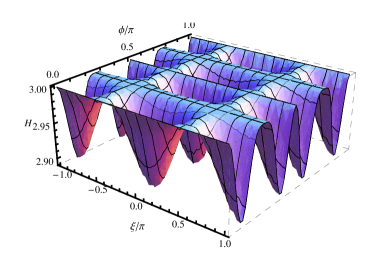
Figure 4: Entropy of three-letter words ($H$ in bits) as a function of the measurement parameters $\xi$ and $\phi$. The entropy attains the maximum 3 for $\phi=k\,\pi/4$.

5.4 Sequential readout of matrix-product states

In this section we show that the statistics of sequential measurements on some matrix-product-states (MPS) (see [19] and references therein) can be simulated by HQMM. More specifically, we concentrate on translationally-invariant open boundary condition MPS with bond dimension $D$, of a many-body state $|\psi\rangle\in\mathcal{H}_{\mathcal{B}}^{\otimes n}$ of the form

$$|\psi\rangle=\sum_{i_{1},\ldots,i_{n}}V_{[n]}^{i_{n}}\cdots V_{[1]}^{i_{1}}|i_{n},\ldots,i_{1}\rangle,$$ (59)

where $i_{k}$ runs from 1 to $d=\dim\mathcal{H}_{\mathcal{B}}$ and $V^{i}_{[k]},~{}1<k<n$ are $D\times D$ matrices and the first and last are row and column vectors, respectively. In [20, 19] it is shown that every MPS of the form of Eq. 59) can be generated sequentially by isometries $\mathcal{H}_{\mathcal{A}}\rightarrow\mathcal{H}_{\mathcal{A}}\otimes\mathcal{H}_{\mathcal{B}}$ of dimension $dD\times D$, with the constraint that the last isometry decouples the spin chain $\mathcal{H}_{\mathcal{B}}^{\otimes n}$ from the system $\mathcal{H}_{\mathcal{A}}$. The isometries are of the form

$$V=\sum_{i,\alpha,\beta}V^{i}_{\alpha,\beta}|\alpha,i\rangle\langle\beta|,$$ (60)

and the assuming that $|\psi\rangle=\langle\psi_{F}|\tilde{V}_{[n]}\cdots\tilde{V}_{[1]}|\psi_{I}\rangle$. Here greek indices refer to dimensions on system $\mathcal{A}$ and latin indices refer to system $\mathcal{B}$, and $|\psi_{I}\rangle$ and $|\psi_{F}\rangle$ are initial and final states of system $\mathcal{A}$, respectively. Since we are interested in generating stochastic processes with arbitrarily long sequences, we will only be concerned with the initial state. The final state will not enter our discussion. Moreover, translational invariance of the MPS representation means that all matrices $V^{i}_{[k]}$ are independent of the site index, $k$. We therefore we drop it from now on .

A more physically intuitive picture arises by considering the isometries as entangling unitary transformations $\mathcal{V}$ between system $\mathcal{A}$ and system $\mathcal{B}$ in an initialized state $|0\rangle\in\mathcal{H}_{\mathcal{B}}$, such that when acting on an initialized ancilla yields

$$\mathcal{V}|0\rangle=\sum_{i\alpha\beta}V^{i}_{\alpha,\beta}|\alpha,i\rangle\langle\beta|.$$ (61)

A note about semantics is in order. In the original paper [20] the term ancilla refers to system $\mathcal{A}$ whereas in our language we consider system $\mathcal{B}$ to be the ancilla. This is because in the literature, concern is focused in generating multipartite quantum states, and system $\mathcal{A}$ only assists in this process. Instead, in our approach, system $\mathcal{B}$ is considered only as an assistance for implementing generalized measurements on $\mathcal{A}$, hence we call $\mathcal{B}$ the ancilla.

Now, after $k$th ancilla $\mathcal{B}$ has been involved in the corresponding isometry, it can be measured, just like in the example of Sec. 5.2. Let $\rho$ be the state of the system prior to step $k$. Attaching the initialized ancilla and performing the entangling operation yields $\mathcal{V}\,(\rho_{k-1}\otimes|0\rangle\langle 0|)\,\mathcal{V}^{\dagger}$. Now, performing a projective measurement on system $\mathcal{B}$ yields

$$\rho_{s}=\tr_{\mathcal{B}}\big{[}(\mathbb{I}\otimes P_{s})\mathcal{V}\,(\rho\otimes|0\rangle\langle 0|)\,\mathcal{V}^{\dagger}(\mathbb{I}\otimes P_{s})\big{]}$$ (62)

By defining the quantum operation $\mathcal{K}_{s}\cdot=\sum_{i}K_{s}^{i}\cdot K_{s}^{i}{}^{\dagger}$ with

$$K_{s}^{i}=\langle i|P_{s}\mathcal{V}|0\rangle=\sum_{\alpha\beta j}\langle i|P_{s}|j\rangle\,[V]^{j}_{\alpha\beta}\,|\alpha\rangle\langle\beta|,$$ (63)

we can write

$$\rho_{s}=\mathcal{K}_{s}\rho,$$ (64)

while

$$\sum_{i,s}K_{s}^{i}{}^{\dagger}K_{s}^{i}=\mathbb{I},$$ (65)

showing that $\{\mathcal{K}_{s}\}$ a well defined stochastic quantum operation.

This shows that, although arbitrary MPS states will require specific initial and final isometries (initialization of system $|\psi_{I}\rangle$ and decoupling in the last step, $|\psi_{F}\rangle$), we are only interested in long sequences of outcomes for arbitrarily large MPS, and hence we can disregard the final decoupling step. Therefore HQMMs can generate the same measurement statistics as sequential identical measurements on any many-body state that admits a translationally invariant MPS representation

$$|\psi\rangle=\sum_{i_{1}\ldots i_{n}}\langle\psi_{F}|V^{i_{n}}\cdots V^{i_{1}}|\psi_{I}\rangle\,|i_{n}\ldots i_{1}\rangle\,.$$ (66)

The number of internal states of the required HQMMcorresponds to the bond dimension $D$ of such MPS representation. The study of random processes generated by HQMMs should then be highly connected to the results on correlation lengths and other properties of certain many-body systems. To the best of our knowledge, this establishes a –yet unexplored– two-way communication between the theory of many-body states and the theory of stochastic processes.

6 An example where quantum outperforms classical

After showing that HQMMs provide a convenient framework to model stochastic processes generated by a variety of quantum systems, it is reasonable to ask whether a more efficient description of a given stochastic process is allowed in the quantum formalism as compared to the classical case. A general answer to this question is beyond the scope of this paper. However, we will provide evidence that some stochastic processes admit a simpler representation within the quantum formalism. For this we present a 4-state classical model, and show that it cannot be reduced to fewer than three states. Then we provide a 2-state HQMM that generates the same process.

Consider the 4-symbol stochastic process ($s\in\{0,1,2,3\}$) given by (states labeled in the order $U,D,R,L$)

$$T_{0} =\left({\small\begin{array}[]{cccc}1/2&0&1/4&1/4\\ 0&0&0&0\\ 0&0&0&0\\ 0&0&0&0\end{array}}\right),\quad T_{1}=\left({\small\begin{array}[]{cccc}0&0&0&0\\ 0&1/2&1/4&1/4\\ 0&0&0&0\\ 0&0&0&0\end{array}}\right)\,,$$ (75)

$$T_{2} =\left({\small\begin{array}[]{cccc}0&0&0&0\\ 0&0&0&0\\ 1/4&1/4&1/2&0\\ 0&0&0&0\end{array}}\right),\quad T_{3}=\left({\small\begin{array}[]{cccc}0&0&0&0\\ 0&0&0&0\\ 0&0&0&0\\ 1/4&1/4&0&1/2\end{array}}\right).~{}~{}~{}~{}~{}~{}$$ (84)

and is depicted in Fig. 5.

Figure 5: Diagrammatic representation of the stochastic generator for the HQMM defined by (75).

A simple method for obtaining a lower bound to the number of internal states necessary for representing a given HMM was provided in [21]. This bound may turn out to be too loose, since positivity and other conditions are not enforced. However, it will suffice to make our point. In our argument we follow closely the approach in [21]. Suppose the statistics of the model (75) can be obtained from a HMM with $n$ internal states. Then, consider the matrix

$$H=\left(\begin{array}[]{lllll}\mathrm{Pr}(\emptyset)&\mathrm{Pr}(0)&\mathrm{Pr}(1)&\mathrm{Pr}(2)&\mathrm{Pr}(3)\\ \mathrm{Pr}(0)&\mathrm{Pr}(00)&\mathrm{Pr}(10)&\mathrm{Pr}(20)&\mathrm{Pr}(30)\\ \mathrm{Pr}(1)&\mathrm{Pr}(01)&\mathrm{Pr}(11)&\mathrm{Pr}(21)&\mathrm{Pr}(31)\\ \mathrm{Pr}(2)&\mathrm{Pr}(02)&\mathrm{Pr}(12)&\mathrm{Pr}(22)&\mathrm{Pr}(32)\\ \mathrm{Pr}(3)&\mathrm{Pr}(03)&\mathrm{Pr}(13)&\mathrm{Pr}(23)&\mathrm{Pr}(33)\end{array}\right).$$ (85)

This is the upper-left corner of an infinite matrix known in the literature as the Hankel matrix. By convention it is assumed that $\mathrm{Pr}(\emptyset)=1$. Expanding the structure of $\mathrm{Pr}(s_{1}s_{2})=\langle 1|T_{s_{2}}T_{s_{1}}|\pi\rangle$ we can write

$$H=\left(\begin{array}[]{l}\langle 1|T_{\emptyset}\\ \langle 1|T_{0}\\ \langle 1|T_{1}\\ \langle 1|T_{2}\\ \langle 1|T_{3}\\ \end{array}\right)\left(\begin{array}[]{lllll}T_{\emptyset}|\pi\rangle&T_{0}|\pi\rangle&T_{1}|\pi\rangle&T_{2}|\pi\rangle&T_{3}|\pi\rangle\end{array}\right),$$ (86)

where $T_{\emptyset}=\mathbb{I}$. Notice that each block in this factorization is a vector of dimension $n$. Therefore the rank of both the left and the right matrices in Eq. (86) are bounded by $n$. Since $H$ and all similar subblocks are factorized in the same manner, any sublock of the Hankel matrix, and in particular that shown in Eq. (85), cannot have rank higher than $n$. Assuming that $n$ could be reduced to 2, we are thus led to the conclusion that $\textrm{rank}(H)\leq 2$. It is now straightforward to explicitly compute $\textrm{rank}(H)$. For this, use Eq. (75) together with $\sum_{s}T_{s}|\pi\rangle=|\pi\rangle$, with $|\pi\rangle=\frac{1}{4}|1\rangle$. Then

$$\textrm{rank}(H)=\textrm{rank}\left(\begin{array}[]{lllll}1&\frac{1}{4}&\frac{1}{4}&\frac{1}{4}&\frac{1}{4}\\ \frac{1}{4}&\frac{1}{8}&0&\frac{1}{16}&\frac{1}{16}\\ \frac{1}{4}&0&\frac{1}{8}&\frac{1}{16}&\frac{1}{16}\\ \frac{1}{4}&\frac{1}{16}&\frac{1}{16}&\frac{1}{8}&0\\ \frac{1}{4}&\frac{1}{16}&\frac{1}{16}&0&\frac{1}{8}\end{array}\right)=3\,.$$ (87)

This shows that the model described in Eq. (75) cannot be implemented by a two-state HMM. It is, however, generated by a HQMMdescribed by ($\mathcal{K}_{y}\cdot=K_{y}\cdot K_{y}^{\dagger}$):

$$K_{0} = \frac{1}{\sqrt{2}}|\uparrow\rangle\langle\uparrow|,\qquad K_{2}=\frac{1}{\sqrt{2}}|+\rangle\langle+|\,,$$

$$K_{1} = \frac{1}{\sqrt{2}}|\downarrow\rangle\langle\downarrow|,\qquad K_{3}=\frac{1}{\sqrt{2}}|-\rangle\langle-|\,.$$ (88)

Indeed, the HMM in Eq. (75) can easily be derived from the HQMM in Eq. (6).

7 Discussion

We have introduced Hidden Quantum Models, inspired by the success of Hidden Markov Models in modelling a wide variety of relevant stochastic processes, and by the natural analogy that exists between the latter and the modern formalism of Quantum Mechanics. We expect HQMMs to provide a wide framework which allows to systematically study quantum processes in which the access to the quantum system is limited, and measurements are constrained to some constant and sequential leaking of classical information. We have considered the least restrictive approach and considered most general CP maps which describe not only the outcome statistics of the measurements but also the effect on the quantum system. These models are a generalization to previously considered classical automata, such as stochastic generators, Mealy automata and hidden Markov models. At the same time, our models generalize the class of quantum generators considered previously in the literature. The advantages of considering HQMMs are many-fold. On the one hand, it is sufficiently general to naturally encompass all Hidden Markov Models, a highly desirable feature for any quantum model attempting to outperform their classical counterpart. On the other hand, they provide the most compressed description of a quantum process by only accounting for the dynamics of the relevant part of the system, i.e., that which contains the quantum information latent in the system.

We foresee a number of questions related to HQMMs with practical and theoretical relevance. We have shown that HQMMs can provide a reduction of the necessary number of internal states necessary for generating some stochastic processes, as compared with classical generators. It is then natural to ask to what extent does this reduction take place, i.e., whether a significant reduction of the resources can take place, or classical generators only require a polynomial overhead on the resources required by HQMMs. On a related ground, HQMMs are fit to describe processes which are simple enough to be considered repetitive, but have an unavoidable quantum essence. It is interesting to ask whether the dimensionality of the quantum system induces some limitations on the generated stochastic processes. This would certainly have implications such as fundamental dimensionality tests for quantum systems under limited accessing freedom. Moreover, in sight of the relation between HQMMs and MPS, unraveling the capabilities and limitations of HQMMs may yield insight on the role of adaptivity in measurement-based quantum computation.

On a more applied level, it is worth noticing that a well established theory of inference exists for HMMs [22, 23]. This can be roughly divided in two classes, namely, state inference and parameter inference. Both of these have close cousins in the field of quantum metrology [24, 25]. It is natural to ask to what extent can these tools be adapted for addressing questions regarding HQMMs, such as those collected in [23]. It is worth mentioning that some of these questions have already triggered interest within the quantum information community [26].

Acknowledgment.

The authors wish to thank useful discussions with E. Bagan, J. Calsamiglia, R. Muñoz-Tapia and M. Plenio. A.M. acknowledges finnancial support from the European Commission of the European Union under the FP7 STREP Project HIP (Hybrid Information Processing), Grant Agreement n. 221889, from MIUR under the FARB fund, from INFN under Iniziativa Specifica PG 62, from CNR-INFM Center Coherentia and from the UK Engineering and Physical Sciences Research Council through the QIP IRC. A.B. thanks the Royal Society and the GCHQ for their support through a James Ellis University Research Fellowship. KW acknowledges funding through EPSRC grant EP/E501214/1.

References

References

- [1] P. Shor, Polynomial-time algorithms for prime factorization and discrete logarithms on a quantum computer, Proceedings of the 35th Annual Symposium on Foundations of Computer Science, p. 124 (1994).
- [2] L. K. Grover, A fast quantum mechanical algorithm for database search, 28th Annual ACM Symposium on the Theory of Computation, p. 212 (1996).
- [3] E. Knill, R. Laflamme, R. Martinez, and C.-H. Tseng, An algorithmic benchmark for quantum information processing, Nature 404, 368 (2000).
- [4] K. Wiesner and J. P. Crutchfield, Computation in finitary stochastic and quantum processes, Physica D 237, 1173 (2008).
- [5] J. P. Crutchfield and K. Wiesner, Intrinsic quantum computation, Phys. Lett. A 372, 375 (2008).
- [6] K. Kraus, Operations and effects in the Hilbert space formulation of quantum theory, p. 206 Springer (1974).
- [7] A. Paz, Introduction to Probabilistic Automata, Academic Press Inc., U.S. (1971).
- [8] P. Grassberger, Toward a quantitative theory of self-generated complexity, Int. J. Theor. Phys. 25, 907 (1986).
- [9] J. P. Crutchfield and K. Young, Inferring statistical complexity, Phys. Rev. Lett. 63, 105 (1989).
- [10] T. M. Cover and J. A. Thomas, Elements of Information Theory, 2nd edition, Wiley- Interscience (2006).
- [11] M. Li and P. Vitanyi, An Introduction to Kolmogorov Complexity and Its Applications, 2nd edition Springer (1997).
- [12] B. Weiss, Subshifts of finite type and sofic systems, Monastsh. Math. 77, 462 (1973).
- [13] B. P. Kitchens, Symbolic Dynamics: One-Sided, Two-Sided and Countable State Markov Shifts, p. 143 Springer (1997).
- [14] M. A. Nielsen and I. L. Chuang, Quantum Computation and Quantum Information, Cambridge University Press, 1st edition (2000).
- [15] [15] K. E. Hellwig and K. Kraus. Pure operations and measurements. Communications in Mathematical Physics 11, 214 (1969).
- [16] K. E. Hellwig and K. Kraus, Operations and measurements. ii. Communications in Mathematical Physics, 16, 142 (1970).
- [17] I. Bengtsson and K. Zyczkowski, Geometry of Quantum States: An Introduction to Quantum Entanglement, Cambridge University Press, 1st edition (2006).
- [18] H. J. Briegel and R. Raussendorf, Persistent entanglement in arrays of interacting particles, Phys. Rev. Lett. 86, 910 (2001).
- [19] D. Perez-Garcia, F. Verstraete, M. M. Wolf, and J. I. Cirac, Matrix product state representations, Quantum Inf. and Comp. 7, 401 (2007).
- [20] C. Schön, E. Solano, F. Verstraete, J. I. Cirac, and M. M. Wolf, Sequential generation of entangled multiqubit states, Phys. Rev. Lett. 95, 110503 (2005).
- [21] B. D. O. Anderson, The realization problem for hidden markov models, Mathematics of Control, Signals, and Systems (MCSS) 12, 80 (1999).
- [22] T. Hastie, R. Tibshirani, and J. Friedman, The Elements of Statistical Learning: Data Mining, Inference, and Prediction 2nd edition, Springer (2009).
- [23] O. Capp’e, E. Moulines, and T. Ryden, Inference in Hidden Markov Models Springer (2007).
- [24] C. W. Helstrom, Quantum Detection and Estimation Theory, Academic Press Inc., U.S. (1976).
- [25] A. S. Holevo, Statistical Structure of Quantum Theory 1st edition, Springer (2001).
- [26] B. Juba, On learning Finite-State quantum sources, arXiv:0910.3713 (2009).