Abstract

The possibility of realizing the superradiant regime of electromagnetic emission by the assembly of quantum dots is considered. The overall dynamical process is analyzed in detail. It is shown that there can occur several qualitatively different stages of evolution. The process starts with dipolar waves triggering the spontaneous radiation of individual dots. This corresponds to the fluctuation stage, when the dots are not yet noticeably correlated with each other. The second is the quantum stage, when the dot interactions through the common radiation field become more important, but the coherence is not yet developed. The third is the coherent stage, when the dots radiate coherently, emitting a superradiant pulse. After the superradiant pulse, the system of dots relaxes to an incoherent state in the relaxation stage. If there is no external permanent pumping, or the effective dot interactions are weak, the system tends to a stationary state during the last stationary stage, when coherence dies out to a low, practically negligible, level. In the case of permanent pumping, there exists the sixth stage of pulsing superradiance, when the system of dots emits separate coherent pulses.

PACS numbers: 73.21.La, 73.21.Fg, 78.67.Hc, 78.67.De

1 Introduction

Superradiance is the effect of self-organized collective coherent radiation by an ensemble of radiators. The phenomenon of optical superradiance is well known for atoms and molecules, being described in numerous publications (see., e.g., books [1-3]). Optical superradiance from Bose-Einstein condensed atoms has also been investigated [4]. There also exists spin superradiance produced by spin systems, such as nuclei [5-8] or magnetic molecules [9-12]. It has been suggested [13] that the assemblies of quantum dots or wells could also be arranged so that to produce superradiance. This can become possible when the distance between the neighboring quantum nanostructures is smaller than the radiation wavelength. In that case, there appears an effective interaction between the radiators, due to common radiation field. The modern technology of preparing materials with quantum dots allows for the fabrication of the quantum dot assemblies with the density of quantum dots sufficient for the appearance of such an effective interaction [13-17], which has been detected experimentally [18].

Quantum dots, whose electrons or holes are confined in all three spatial dimensions, have many properties [19-22] that make them similar to atoms, because of which quantum dots are often called ”artificial atoms”. One of the main such properties is the existence of discrete energy levels, whose shell structure can be adjusted by design. Some of these properties are shared by quantum wells confining electrons or holes in one dimension and allowing free propagation in two dimensions. For concreteness, we shall concentrate in what follows on the consideration of quantum dots.

Transferring electrons from the ground-state energy level to an excited level creates a hole. The interacting pair of an excited electron and a hole forms an exciton. The electron-hole recombination is accompanied by the radiation of electromagnetic field, which is in a very close analogy with the radiation of excited atoms. This is why it was reasonable to assume [23] that an ensemble of quantum dots can be employed for the creation of quantum-dot lasers. Several types of quantum-dot lasers have been demonstrated since then, based on semiconductor heterojunctions [24-29] and photonic crystals [30-33]. Quantum-well lasers have also been realized. But the latter, because of thermal occupation of the the quasi-2D continuum, are essentially more sensitive to temperature changes, which makes their emission less monochromatic than that of quantum dots. Quantum-dot lasers also enjoy a lower current-density lasing threshold. Because of these differences, quantum dots look more suitable for the use as radiating devices.

When quantum dots are fabricated in the process of epitaxial growth, they are usually characterized by a noticeable size dispersion, which results in the related inhomogeneous broadening. The latter may hinder the possibility of achieving efficient dot interactions through the common radiation field and, as a result, destroying the cooperative character of emission, thus, suppressing coherence [15,34,35]. However the impressive recent progress in controlling quantum-dot parameters [18,27] makes it now feasible to create quantum dots so that they allow for the appearance of effective dot interactions through electromagnetic field, which is a prerequisite for achieving collective coherent radiation.

Because of the technological feasibility of fabricating semiconductor samples with sufficiently dense and uniform quantum dots, it should be possible to realize the conditions for their superradiant emission. It is the aim of the present paper to consider the quantum-dot superradiance. The main goal is to develop an accurate and detailed description of all stages of the superradiant dynamics, starting from the initial stage, when collective effects are yet weak, to the coherent stage of radiation, and further to the end of the whole process. The developed theory makes it possible to describe different types of superradiance, such as pure superradiance, triggered superradiance, and pulsing superradiance.

The aim of the paper is to consider the realistic situation corresponding to quantum dots, but not an oversimplified model consideration. Therefore, in order to understand what approximations are admissible for characterizing the process, in the next section, an analysis of the parameters, typical of semiconductors with quantum dots, will be given. Such an analysis is necessary before plunging into mathematical formulas in the following sections. The parameters are taken from the literature cited above.

2 Typical Material Parameters

For realizing quantum-dot superradiance, it is reasonable to take those materials that are used for quantum-dot lasers. For the latter, one usually employs the self-assembled heterostructures, such as InAs/GaAs, InGaAs/GaAs, InGaAs/AlGaAs, GaInAsP/InP, InAs/InP, InAs/GaInAs, AlInAs/AlGaAs, InP/GaInP, AlGaAs/GaAs, and CdSe/ZnSe. There exist different kinds of quantum dots, having different shapes and sizes. Thus, the lateral size of a typical self-assembled quantum dot is much larger than its vertical extent. Typical dot sizes are of the order $r_{dot}\sim 10^{-7}cm-10^{-6}cm$. In each dot, there can be between just a few to $10^{5}$ electrons. The dot density in an epitaxy layer is of order $10^{8}cm^{-2}-10^{11}cm^{-2}$. With the width of the layer $h\sim 10^{-6}cm-10^{-5}cm$, this makes the spatial density $\rho\sim 10^{13}cm^{-3}-10^{17}cm^{-3}$. The interdot distance is $a\sim 10^{-5}cm-10^{-4}cm$. The lasing operation is realized at the wavelength $\lambda\sim 10^{-4}cm$, which translates into the frequency $\omega_{0}\sim 10^{15}Hz$. The natural width $\gamma_{0}=2|d|^{2}k_{0}^{3}/3$, where $k_{0}=2\pi/\lambda$, depends on the transition dipole $d$. The typical value for the latter is $d\sim 100D$. Taking into account that $1D=10^{-17}\sqrt{erg\cdot cm^{3}}$ gives $\gamma_{0}\sim 10^{10}Hz$. The actual homogeneous broadening is usually larger than $\gamma_{0}$, being $\gamma_{2}\sim 10^{12}Hz-10^{13}Hz$. For high-quality self-assembled dot materials, the inhomogeneous broadening can be made relatively small, of the same order as $\gamma_{2}$, that is, of order $\gamma_{2}^{*}\sim 10^{12}Hz-10^{13}Hz$. The longitudinal relaxation time $T_{1}$ is mainly due to electron-phonon coupling, which can be strongly suppressed by low temperatures. Thus, at helium temperatures, the longitudinal dephasing time becomes limited only by the lifetime of inversion for a single quantum dot in free space, $T_{1}\sim 10^{-9}s$, which gives $\gamma_{1}\equiv 1/T_{1}\sim 10^{9}Hz$. To enhance a chosen mode, one places the sample into a resonator cavity with a large quality factor reaching $10^{4}$. The sizes of the sample can be different. Edge-emitting lasers do not have a circular cross-section. The typical sizes of quantum dot lasers can be $R\sim 10^{-3}cm-10^{-2}cm$.

Since the radiation wavelength is much larger than the dot sizes, $\lambda\gg r_{dot}$, the dipole approximation is appropriate. For sufficiently dense dot materials, the interdot distance can be made much smaller than the wavelength, $a\ll\lambda$. Hence, there can arise sufficiently strong dot interaction through the common radiation field. But the wavelength is much smaller than the sample linear sizes, $\lambda\ll L$. Therefore the Dicke-type [36] approximation of a concentrated, point-like, sample, cannot be used. In strongly nonuniform materials, with a very large inhomogeneous broadening $\gamma_{2}^{*}$, such that $T_{2}^{*}\equiv 1/\gamma_{2}^{*}$ is comparable with the time of the radiation pulse $\tau_{p}$, superradiance is suppressed [34]. It is therefore necessary to prepare the samples with a narrow distribution of dot sizes, resulting in not too wide inhomogeneous broadening. Fortunately, the fabrication of such samples is nowadays technologically possible. As is seen from the above values for typical parameters, the inhomogeneous broadening can be made of the same order as the homogeneous one. When $\gamma_{2}^{*}\sim\gamma_{2}$, then the consideration can be simplified by combining $\gamma_{2}^{*}$ and $\gamma_{2}$ in one effective parameter [37]. Thus, the typical dephasing time is rather short, $T_{2}\equiv 1/\gamma_{2}\sim 10^{-13}s-10^{-12}s$. Superradiance is possible only if the time of radiation pulse $\tau_{p}$ is shorter than the dephasing time $T_{2}$. In the following sections, the theoretical description is developed, which takes into account the typical characteristics of the quantum dot assemblies. Throughout the paper, the system of units is used, where the Planck constant $\hbar\equiv 1$.

3 Basic Operator Equations

Aiming at developing a realistic description of the system, let us start with the microscopic Hamiltonian

$$\hat{H}=\hat{H}_{d}+\hat{H}_{f}+\hat{H}_{df}+\hat{H}_{mf}\;,$$ (1)

characterizing an ensemble of radiating quantum dots in a semiconductor matrix inside a resonator cavity. The Hamiltonian

$$\hat{H}_{d}=\sum_{i=1}^{N}\omega_{0}\left(\frac{1}{2}+S_{i}^{z}\right)\;,$$ (2)

where $S_{i}^{z}$ is a pseudospin operator of an $i$-th dot, represents $N$ two-level quantum dots, with the carrying transition frequency $\omega_{0}$. Mathematically, the operator $S_{i}^{z}$ is just a spin operator. It is called the pseudospin operator, since it corresponds not to an actual spin but to the population difference. The radiation-field Hamiltonian

$$\hat{H}_{f}=\frac{1}{8\pi}\int\left({\bf E}^{2}+{\bf H}^{2}\right)\;d{\bf r}\;,$$ (3)

contains electric field $\bf E$ and magnetic field $\bf H$. The vector potential ${\bf A}$, introduced by the standard relation ${\bf H}=\nabla\times{\bf A}$, is assumed to satisfy the Coulomb calibration $\nabla\cdot{\bf A}=0$. The dot-field interaction is given by the Hamiltonian

$$\hat{H}_{df}=-\sum_{i=1}^{N}\left(\frac{1}{c}\;{\bf J}_{i}\cdot{\bf A}_{i}+{\bf P}_{i}\cdot{\bf E}_{0i}\right)\;,$$ (4)

in which ${\bf A}_{i}\equiv{\bf A}({\bf r}_{i},t)$ and ${\bf E}_{0i}\equiv{\bf E}_{0}({\bf r}_{i},t)$ is a seed electric field of the resonator cavity. The transition current

$${\bf J}_{i}=i\omega_{0}\left({\bf d}S_{i}^{+}-{\bf d}^{*}S_{i}^{-}\right)\;,$$ (5)

and transition polarization

$${\bf P}_{i}={\bf d}S_{i}^{+}+{\bf d}^{*}S_{i}^{-}\;,$$ (6)

are expressed through the transition dipole $\bf d$ and the ladder operators $S_{i}^{\pm}\equiv S_{i}^{x}\pm iS_{i}^{y}$, where $S_{i}^{\alpha}\equiv S^{\alpha}({\bf r}_{i},t)$. Since the cavity is filled by a semiconducting material, the Hamiltonian

$$\hat{H}_{mf}=-\;\frac{1}{c}\int{\bf j}_{mat}({\bf r},t)\cdot{\bf A}({\bf r},t)\;d{\bf r}\;,$$ (7)

describes the interaction of the local density current $j_{mat}({\bf r},t)$ in the filling matter with the radiated electromagnetic field.

The field operators satisfy the equal-time commutation relations

$$\left[E^{\alpha}({\bf r},t),\;A^{\beta}({\bf r}^{\prime},t)\right]=4\pi ic\delta_{\alpha\beta}({\bf r}-{\bf r}^{\prime})\;,$$

$$\left[E^{\alpha}({\bf r},t),\;H^{\beta}({\bf r}^{\prime},t)\right]=-4\pi ic\sum_{\gamma}\varepsilon_{\alpha\beta\gamma}\;\frac{\partial}{\partial r^{\gamma}}\;\delta({\bf r}-{\bf r}^{\prime})\;,$$ (8)

where $\epsilon_{\alpha\beta\gamma}$ is the unitary antisymmetric tensor [3] and the transverse delta-function is

$$\delta_{\alpha\beta}({\bf r})\equiv\int\left(\delta_{\alpha\beta}\;-\;\frac{k^{\alpha}k^{\beta}}{k^{2}}\right)e^{i{\bf k}\cdot{\bf r}}\;\frac{d{\bf k}}{(2\pi)^{3}}=\frac{2}{3}\;\delta_{\alpha\beta}\delta({\bf r})\;-\;\frac{1}{4\pi}\;D_{\alpha\beta}({\bf r})\;,$$ (9)

with the dipolar tensor

$$D_{\alpha\beta}({\bf r})\equiv\frac{\delta_{\alpha\beta}-3n^{\alpha}n^{\beta}}{r^{3}}\;,$$

in which ${\bf n}\equiv{\bf r}/r=\{n^{\alpha}\}$ and $r\equiv|\bf r|$. The pseudospin operators satisfy the spin commutation relations

$$\left[S^{+}_{i},\;S_{j}^{-}\right]=2\delta_{ij}S_{i}^{z}\;,\qquad\left[S^{z}_{i},\;S_{j}^{\pm}\right]=\pm\delta_{ij}S_{i}^{\pm}\;.$$ (10)

The Heisenberg equations of motion for the field operators yield

$$\frac{1}{c}\;\frac{\partial{\bf E}}{\partial t}=\nabla\times{\bf H}\;-\;\frac{4\pi}{c}\;{\bf j}\;,\qquad\frac{1}{c}\;\frac{\partial{\bf A}}{\partial t}=-{\bf E}\;,$$ (11)

with the density of current

$$j^{\alpha}({\bf r},t)=\sum_{\beta}\left[\sum_{i=1}^{N}\delta_{\alpha\beta}({\bf r}-{\bf r}_{i})J_{i}^{\beta}(t)+\int\delta_{\alpha\beta}({\bf r}-{\bf r}^{\prime})j_{mat}^{\beta}({\bf r}^{\prime},t)\;d{\bf r}^{\prime}\right]\;.$$ (12)

¿From these, using the Coulomb calibration, one gets the equation for the vector potential

$$\left(\nabla^{2}\;-\;\frac{1}{c^{2}}\;\frac{\partial^{2}}{\partial t^{2}}\right){\bf A}=-\;\frac{4\pi}{c}\;{\bf j}\;.$$ (13)

The Heisenberg equations for the pseudospin operators result in the equations

$$\frac{dS_{i}^{-}}{dt}=-i\omega_{0}S_{i}^{-}+2S_{i}^{z}\left(k_{0}{\bf d}\cdot{\bf A}_{i}-i{\bf d}\cdot{\bf E}_{0i}\right)\;,$$

$$\frac{dS_{i}^{z}}{dt}=-S_{i}^{+}\left(k_{0}{\bf d}\cdot{\bf A}_{i}-i{\bf d}\cdot{\bf E}_{0i}\right)-S_{i}^{-}\left(k_{0}{\bf d}^{*}\cdot{\bf A}_{i}+i{\bf d}^{*}\cdot{\bf E}_{0i}\right)\;,$$ (14)

where $k_{0}=\omega_{0}/c$. These equations are to be complimented by the retardation condition

$$S_{i}^{\alpha}(t)=0\qquad(t<0)\;.$$ (15)

Equations (11) to (15) are the basic operator equations describing all radiation processes in the system of quantum dots. It is worth emphasizing that these equations follow from the first principles. Such a microscopic approach is necessary for correctly treating the overall dynamics of quantum dot radiation.

4 Elimination of Field Variables

The standard way of considering the radiation processes is by averaging Eqs. (11) and (14) and passing to the semiclassical approximation. This way, presupposing well organized coherence, does not allow for the treatment of those radiation stages, when coherence has not been developed. Therefore, we employ here another, more accurate, approach allowing for the treatment of all radiation stages.

The first step in the approach to be pursued is the elimination of field variables [8]. This can be done by solving Eq. (13) for the vector potential and substituting the found solution into Eqs. (14) for the pseudospin operators. The known solution of Eq. (13) is the sum

$${\bf A}({\bf r},t)={\bf A}_{vac}+\frac{1}{c}\int{\bf j}\left({\bf r}^{\prime},t-\;\frac{|{\bf r}-{\bf r}^{\prime}|}{c}\right)\;\frac{d{\bf r}^{\prime}}{|{\bf r}-{\bf r}^{\prime}|}$$ (16)

of the vacuum potential and the retarded potential, with the density of current given by Eq. (12). This solution is to be substituted into Eqs. (14).

The interaction between the radiation field and a radiating dot is assumed to be small as compared to the transition frequency. This is a necessary requirement for the existence of well defined energy levels in a dot. In the other case, the transition frequency would not be defined in principle. This implies that the retardation in the time dependence of the current density can be taken into account in the Born approximation

$$S_{j}^{-}\left(t-\frac{r}{c}\right)=S_{j}^{-}(t)\Theta(ct-r)e^{ik_{0}r}\;,\qquad S_{j}^{z}\left(t-\frac{r}{c}\right)=S_{j}^{z}(t)\Theta(ct-r)\;,$$

where $\Theta(t)$ is the unit step function.

When substituting the vector potential (16) into Eqs. (14), one meets the terms corresponding to the dot self-action. The contribution of these terms is characterized in the Appendix. Finally, the vector potential (16) is represented as the sum

$${\bf A}={\bf A}_{vac}+{\bf A}_{self}+{\bf A}_{rad}+{\bf A}_{dip}+{\bf A}_{mat}\;.$$ (17)

Here the first term is due to vacuum fluctuations. The self-action potential is described in the Appendix. The radiation potential

$${\bf A}_{rad}({\bf r},t)=\sum_{j}\;\frac{2}{3c|{\bf r}-{\bf r}_{j}|}\;{\bf J}_{j}\left(t-\;\frac{|{\bf r}-{\bf r}_{j}|}{c}\right)\;,$$ (18)

in which ${\bf r}\neq{\bf r}_{j}$, describes the spherical part of the vector potential, corresponding to the radiation field produced by dots. In addition, the radiating dots create the dipolar part of the vector potential

$$A_{dip}^{\alpha}({\bf r},t)=-\sum_{j}\sum_{\beta}\int\frac{D_{\alpha\beta}({\bf r}^{\prime}-{\bf r}_{j})}{4\pi c|{\bf r}-{\bf r}^{\prime}|}\;J_{j}^{\beta}\left(t-\;\frac{|{\bf r}-{\bf r}^{\prime}|}{c}\right)\;d{\bf r}^{\prime}\;.$$ (19)

The interaction of the semiconductor, filling the cavity, with the radiation field produces the potential

$$A_{mat}^{\alpha}({\bf r},t)=\sum_{\beta}\int\frac{\delta_{\alpha\beta}({\bf r}^{\prime}-{\bf r}^{\prime\prime})}{c|{\bf r}-{\bf r}^{\prime}|}\;j_{mat}^{\beta}\left({\bf r}^{\prime\prime},t-\;\frac{|{\bf r}-{\bf r}^{\prime}|}{c}\right)\;d{\bf r}^{\prime}d{\bf r}^{\prime\prime}\;.$$ (20)

Substituting the vector potential (17) into Eqs. (14), we obtain the equations for the pseudospin operators, which do not contain the field variables. Instead, there appear effective dot interactions through the common radiation field.

5 Stochastic Mean-Field Approximation

The dynamics of the system can be characterized by the behavior of the following functions. The transition function

$$u({\bf r}_{i},t)\equiv 2\langle S_{i}^{-}(t)\rangle_{H}$$ (21)

where the angle brackets imply quantum statistical averaging associated with the system Hamiltonian $H$, describes the local effective polarization corresponding to dipole transitions. The coherence intensity

$$w({\bf r}_{i},t)\equiv\frac{2}{N}\;\sum_{j(\neq i)}^{N}\left[\langle S_{i}^{+}(t)S_{j}^{-}(t)\rangle_{H}+\langle S_{j}^{+}(t)S_{i}^{-}(t)\rangle_{H}\right]$$ (22)

is the local characteristic of coherence. The intensity of coherent radiation is proportional to this function. The population difference

$$s({\bf r}_{i},t)\equiv 2\langle S_{i}^{z}(t)\rangle_{H}$$ (23)

defines the local difference of populations for the energy levels of an $i$-dot.

To obtain the evolution equations for functions (21), (22), and (23), we have to average the equations resulting after the substitution of the vector potential (17) into the equations of motion (14). Such equations are not closed. To make them closed, it is necessary to invoke some decoupling for the operator correlation functions. If one resorts to the standard mean-field decoupling, one comes to the usual semiclassical approximation. As is well known, the semiclassical approximation can be used only when the system is in a coherent state or is almost coherent [2,3]. But incoherent regimes cannot be described in this approximation. One of the most interesting questions is how coherence develops in an initially incoherent system. To be able to describe such a regime, it is necessary to employ a more accurate approximation. For this purpose, we shall use the stochastic mean-field approximation employed earlier for describing the dynamics of spin assemblies [5-11] and Bose systems in random fields [38-40].

Let us combine the vacuum, dipole, and matter vector potentials into the sum

$$\xi({\bf r},t)\equiv 2k_{0}{\bf d}\cdot\left({\bf A}_{vac}+{\bf A}_{dip}+{\bf A}_{mat}\right)\;.$$ (24)

The potentials, entering this sum, create local fluctuations of electromagnetic field. Being averaged over space, quantity (24) is practically zero. Therefore Eq. (24), characterizing the strength of local field fluctuations, can be treated as a local random variable. Contrary to this random variable, the radiation potential (18) induces long-range effective interactions between the radiating dots. The long-range radiation potential (18), with current (5), is expressed through the pseudospin operators ${\bf S}_{j}$. Hence the effective interactions, arising between dots, are mathematically similar to long-range spin interactions.

There is a direct similarity between the effective dipole interactions caused by the dipole vector potential (19) and the dipole [5-11] and hyperfine interactions [9-11,41,42] in spin systems, these interactions being treated as stochastic fluctuations playing destructive role by dephasing collective motion. While the effective pseudospin interactions, induced by the radiation potential (18) in quantum dots, are equivalent to the effective interactions produced by the resonator feedback field in spin systems [9-11]. The latter interactions are responsible for the appearance of collective effects in magnetic and ferroelectric samples, including the arising coherence [43]. In spin systems without a resonator feedback field, coherence and, hence, superradiance, cannot develop, being destroyed by the direct dipole interactions [5-11,44,45].

In this way, it is possible to distinguish two types of variables in the system, the random variable $\xi$ describing local field fluctuations and the pseudospin variables ${\bf S}_{j}$ characterizing effective long-range dot interactions. For brevity, we may denote the collection of pseudospins $\{{\bf S}_{j}:j=1,2,...,N\}$ by $\bf S$. Then, the operators of observable quantities $\hat{\cal O}$ are, generally, functions of these variables, $\hat{\cal O}=\hat{\cal O}({\bf S},\xi)$.

Having two kinds of variables, it is possible to define two types of averaging. One type corresponds to the quantum statistical average

$$\langle\hat{\cal O}\rangle_{H}\equiv{\rm Tr}\;\hat{\rho}\;\hat{\cal O}({\bf S},\xi)$$ (25)

involving the pseudospin operators $\bf S$, with $\hat{\rho}$ being the system statistical operator, and where the random variable $\xi$ is kept fixed. Another type is the stochastic averaging over the random fluctuations, denoted as

$$\langle\langle\hat{\cal O}\rangle\rangle\equiv\int\hat{\rho}\;\hat{\cal O}({\bf S},\xi)\;{\cal D}\xi\;,$$ (26)

which is defined through a functional integral over the random variable $\xi$, with the prescribed differential measure ${\cal D}\xi$. Respectively, the total averaging

$$\langle\hat{\cal O}\rangle\equiv\langle\langle\left(\langle\hat{\cal O}\rangle_{H}\right)\rangle\rangle$$ (27)

includes both, the quantum and stochastic, averages.

Keeping in mind the long range of the effective pseudospin interactions, we can use the stochastic mean-field decoupling

$$\langle S_{i}^{\alpha}S_{j}^{\beta}\rangle_{H}=\langle S_{i}^{\alpha}\rangle_{H}\langle S_{j}^{\beta}\rangle_{H}\qquad(i\neq j)\;,$$ (28)

where only the quantum averaging is involved. This decoupling looks like a mean-field approximation. However, it has a very important principal difference form the latter, involving only the quantum averaging (25), but not touching the stochastic averaging (26). Since no approximation is done here with respect to the stochastic variables, decoupling (28) preserves stochastic properties of the system. This is why it is called the stochastic mean-field approximation [5-11].

When the radiation wavelength $\lambda$ is much larger than the interdot distance, the geometrical location of dots in space is of no importance. Then it is convenient to pass to the continuous spatial representation, replacing the sums by the integrals according to the rule

$$\sum_{j=1}^{N}\;\Longrightarrow\;\rho\int d{\bf r}\qquad\left(\rho\equiv\frac{N}{V}\right)\;,$$ (29)

with the integration over the whole system and $\rho$ being the dot density.

In order to represent the evolution equations in a compact form, let us introduce the effective field, or effective force, acting on dots

$$f({\bf r},t)=f_{0}({\bf r},t)+f_{rad}({\bf r},t)+\xi({\bf r},t)\;.$$ (30)

Here, the first term

$$f_{0}({\bf r},t)\equiv-2i{\bf d}\cdot{\bf E}_{0}({\bf r},t)$$ (31)

is due to the external field ${\bf E}_{0}$. The second term

$$f_{rad}({\bf r},t)\equiv 2k_{0}\langle{\bf d}\cdot{\bf A}_{rad}({\bf r},t)\rangle_{H}$$ (32)

is caused by the radiating dots. And the last term in Eq. (30) is the fluctuating random field (24). The radiation term (32), with the vector potential (18), acquires the form

$$f_{rad}({\bf r},t)=-i\gamma_{0}\rho\int\left[G({\bf r}-{\bf r}^{\prime},t)u({\bf r}^{\prime},t)-\;\frac{{\bf d}^{2}}{|{\bf d}|^{2}}\;G^{*}({\bf r}-{\bf r}^{\prime},t)u^{*}({\bf r}^{\prime},t)\right]\;d{\bf r}^{\prime}\;,$$ (33)

in which the transfer kernel is

$$G({\bf r},t)\equiv\frac{\exp(ik_{0}r)}{k_{0}r}\;\Theta(ct-r)\;.$$ (34)

Finally, we average Eqs. (14) according to the quantum averaging (25), employ the stochastic mean-field decoupling (28), and use notation (30). Then for the variables (21), (22), and (23), we obtain the evolution equations

$$\frac{\partial u}{\partial t}=-(i\omega_{0}+\gamma_{2})u+fs\;,\qquad\frac{\partial w}{\partial t}=-2\gamma_{2}w+\left(u^{*}f+f^{*}u\right)s\;,$$

$$\frac{\partial s}{\partial t}=-\;\frac{1}{2}\left(u^{*}f+f^{*}u\right)-\gamma_{1}(s-\zeta)\;,$$ (35)

in which $u=u({\bf r},t),w=w({\bf r},t)$, and $s=s({\bf r},t)$. The longitudinal, $\gamma_{1}$, and transverse, $\gamma_{2}$, attenuation rates are treated as the system parameters, whose typical values are discussed in Sec. II. The parameter $\zeta$ characterizes the level of stationary nonresonant pumping. The evolution equation for $w$ follows from definition (22), with the use of the Heisenberg equations of motion for the pseudospin operators and the stochastic mean-field decoupling (28). Since in definition (22), the summation is over $j\neq i$, it is also possible, first, to decouple the products of the pseudospin operators, according to Eq. (28), and then invoke the Heisenberg equations. In any case, the result is the same equation for $w$.

Equations (35) are stochastic integro-differential equations. These are the basic evolution equations describing the dynamics of radiation in a system of quantum dots.

6 Triggering Dipolar Waves

As is mentioned above, the dipolar vector potential (19) induces local fluctuations dephasing the radiation of the dot assembly. However, these fluctuations play not only destructive role. They can be useful at the initial stage of the radiation process, when the latter is not triggered by an external field. In such a case, the transition dipole fluctuations, related to spontaneous emission, can trigger the process of collective radiation.

In order to illustrate the appearance and the nature of the dipolar fluctuations, let us consider the pseudospin equations (14), leaving there only the terms related to the dipole interactions. Let us introduce the interaction coefficients

$$b_{ij}\equiv\frac{k_{0}^{2}}{2\pi}\;\sum_{\alpha\beta}d^{\alpha}D_{ij}^{\alpha\beta}d^{\beta}\;,\qquad c_{ij}\equiv\frac{k_{0}^{2}}{2\pi}\;\sum_{\alpha\beta}d^{\alpha}\left(D_{ij}^{\alpha\beta}d^{\beta}\right)^{*}\;,$$ (36)

where

$$D_{ij}^{\alpha\beta}\equiv\int\Theta(ct-|{\bf r}_{i}-{\bf r}^{\prime}|)\;\frac{D_{\alpha\beta}({\bf r}^{\prime}-{\bf r}_{j})}{|{\bf r}_{i}-{\bf r}^{\prime}|}\exp(-ik_{0}|{\bf r}_{i}-{\bf r}^{\prime}|)\;d{\bf r}^{\prime}\;.$$

The latter quantity, because of the unit-step function $\Theta(ct-|{\bf r}_{i}-{\bf r}^{\prime}|)$ in the integral, varies in time only at the very beginning of the process, when $t\ll a/c$, after which it becomes practically constant. Therefore, for all times, except $t\ll a/c$, the interaction coefficients (36) can be treated as constant parameters.

For the dipolar vector potential (19), we have

$$k_{0}{\bf d}\cdot{\bf A}_{dip}({\bf r}_{i},t)=-\;\frac{i}{2}\sum_{j(\neq i)}\left[b_{ij}S_{j}^{+}(t)-c_{ij}S_{i}^{-}(t)\right]\;.$$

Then the equations of motion reduce to

$$\frac{dS_{i}^{-}}{dt}=-i\omega_{0}S_{i}^{-}-iS_{i}^{z}\sum_{j(\neq i)}\left(b_{ij}S_{j}^{+}-c_{ij}S_{j}^{-}\right)\;,$$

$$\frac{dS_{i}^{z}}{dt}=\frac{i}{2}\;\sum_{j(\neq i)}\left[S_{i}^{+}\left(b_{ij}S_{j}^{+}-c_{ij}S_{j}^{-}\right)-S_{i}^{-}\left(b_{ij}^{*}S_{j}^{-}-c_{ij}^{*}S_{j}^{+}\right)\right]\;.$$ (37)

The dipolar pseudospin fluctuations are described by the small deviations

$$\delta S_{i}^{\pm}\equiv S_{i}^{\pm}-\langle S_{i}^{\pm}\rangle\;,\qquad\delta S_{i}^{z}\equiv S_{i}^{z}-\langle S_{i}^{z}\rangle$$ (38)

from the related average values $<S_{i}^{\alpha}>$. The latter averages correspond to equilibrium or quasiequilibrium, when they either do not depend on time or are slow functions of time, as compared to the fastly fluctuating deviations (38). Linearizing Eqs. (37) with respect to small deviations (38), under the condition $<S_{i}^{-}>=0$, and taking into account that, because of the properties of dipole interactions,

$$\sum_{j(\neq i)}b_{ij}=\sum_{j(\neq i)}c_{ij}=0\;,$$ (39)

we obtain the equations

$$\frac{d}{dt}\;\delta S_{i}^{-}=-i\omega_{0}\delta S_{i}^{-}-i\langle S_{i}^{z}\rangle\sum_{j(\neq i)}\left(b_{ij}\delta S_{j}^{+}-c_{ij}\delta S_{j}^{-}\right)\;,$$

$$\frac{d}{dt}\;\delta S_{i}^{z}=0\;.$$ (40)

Then we employ the Fourier transforms for the pseudospin operators

$$S_{j}^{\pm}=\sum_{k}S_{k}^{\pm}\exp(\mp i{\bf k}\cdot{\bf r}_{j})\;,\qquad S_{k}^{\pm}=\frac{1}{N}\sum_{j}S_{j}^{\pm}\exp(\pm i{\bf k}\cdot{\bf r}_{j})\;,$$ (41)

for the interaction coefficients

$$b_{ij}=\frac{1}{N}\sum_{k}b_{k}\exp(i{\bf k}\cdot{\bf r}_{ij})\;,\qquad b_{k}=\sum_{j(\neq i)}b_{ij}\exp(-i{\bf k}\cdot{\bf r}_{ij})\;,$$ (42)

and, similarly, for the interaction coefficients $c_{ij}$, where ${\bf r}_{ij}\equiv{\bf r}_{i}-{\bf r}_{j}$. Taking into account that

$$\delta S_{j}^{\pm}=S_{j}^{\pm}\qquad(\langle S_{j}^{\pm}\rangle=0)$$ (43)

and introducing the notation

$$\mu_{k}\equiv\omega_{0}-c_{k}\langle S_{i}^{z}\rangle\;,\qquad\lambda_{k}\equiv b_{-k}\langle S_{i}^{z}\rangle\;,$$ (44)

we come to the equations

$$\frac{dS_{k}^{-}}{dt}=-i\mu_{k}S_{k}^{-}-i\lambda_{k}S_{k}^{+}\;,\qquad\frac{dS_{k}^{+}}{dt}=i\mu_{k}^{*}S_{k}^{+}+i\lambda_{k}^{*}S_{k}^{-}\;.$$ (45)

Looking for the solutions to Eqs. (45) in the form

$$S_{k}^{-}=u_{k}e^{-i\omega_{k}t}+v_{k}^{*}e^{i\omega_{k}t}\;,\qquad S_{k}^{+}=u_{k}^{*}e^{i\omega_{k}t}+v_{k}e^{-i\omega_{k}t}\;,$$ (46)

we find the dipolar-wave spectrum

$$\omega_{k}=\sqrt{|\mu_{k}|^{2}-|\lambda_{k}|^{2}}\;.$$ (47)

This means that the dipolar part (19) of the vector potential generates local field fluctuations, having the meaning of the transition dipolar waves with the spectrum (47). The interaction coefficients (36) are smaller than the transition frequency, so that

$$\frac{|b_{k}|}{\omega_{0}}\ll 1\;,\qquad\frac{|c_{k}|}{\omega_{0}}\ll 1\;.$$ (48)

Hence,

$$\frac{|\lambda_{k}|}{\omega_{0}}\ll 1\;,\qquad\frac{|\lambda_{k}|}{|\mu_{k}|}\ll 1\;.$$ (49)

Therefore the spectrum (47) is always positive, implying that the dipolar waves are dynamically stable [46]. In the long-wave limit, when $k\rightarrow 0$ and

$$b_{k}\simeq-\;\frac{1}{2}\sum_{j(\neq i)}b_{ij}({\bf k}\cdot{\bf r}_{ij})^{2}\;,\qquad c_{k}\simeq-\;\frac{1}{2}\sum_{j(\neq i)}c_{ij}({\bf k}\cdot{\bf r}_{ij})^{2}\;,$$

the spectrum becomes quadratic, which follows from the expression

$$\omega_{k}^{2}\simeq\omega_{0}^{2}+\omega_{0}\langle S_{i}^{z}\rangle\;{\rm Re}\sum_{j(\neq i)}c_{ij}({\bf k}\cdot{\bf r}_{ij})^{2}\;.$$ (50)

The existence of these dipolar waves triggers the process of dot radiation, even if no external field is imposed at the initial time.

7 Transverse Mode Expansion

After the radiation process is triggered by the dipolar waves, the overall radiation dynamics is described by Eqs. (35) that are stochastic integro-differential equations in partial derivatives. If the sizes of the whole sample would be much smaller than the radiation wavelength, we could essentially simplify the problem by resorting to the concentrated-sample approximation [1-3,36], when just one mode fills the cavity. But in realistic situation, vice versa, the wavelength is usually much smaller than the sample sizes, so that the sample can house several modes. Then, to simplify the equations, it is necessary to specify the shape of the resonator cavity.

For concreteness, let us assume that the cavity is cylindrical, with radius $R$ and length $L$, such that the wavelength is much smaller than these sizes:

$$\frac{\lambda}{R}\ll 1\;,\qquad\frac{\lambda}{L}\ll 1\;.$$ (51)

Directing the cylinder axis along the axis $z$, we can treat the resonator seed field as propagating along this axis, that is, having the form

$$E_{0}({\bf r},t)=\frac{1}{2}\;E_{1}e^{i(kz-\omega t)}+\frac{1}{2}\;E_{1}^{*}e^{-i(kz-\omega t)}\;.$$ (52)

The cavity is resonant in the sense of the small detuning of the resonator natural frequency from the dot transition frequency,

$$\frac{|\Delta|}{\omega_{0}}\ll 1\qquad(\Delta\equiv\omega-\omega_{0})\;.$$ (53)

In the same way as it is for all dot-field interactions, for the seed field, we have

$$\frac{|\nu_{1}|}{\omega_{0}}\ll 1\qquad(\nu_{1}\equiv|{\bf d}\cdot{\bf E}_{1}|)\;.$$ (54)

In the cylindrical geometry, the radiation modes acquire the shape of filaments extended along the axis $z$. Then, it is possible to represent the solutions to Eqs. (35) as expansions over the transverse modes:

$$u({\bf r},t)=\sum_{n=1}^{N_{f}}u_{n}(r_{\perp},t)e^{ikz}\;,\qquad w({\bf r},t)=\sum_{n=1}^{N_{f}}w_{n}(r_{\perp},t)\;,$$

$$s({\bf r},t)=\sum_{n=1}^{N_{f}}s_{n}(r_{\perp},t)\;,$$ (55)

where $N_{f}$ is the number of the filamentary modes and $r_{\perp}=\sqrt{x^{2}+y^{2}}$ is the transverse radial variable. Ascribing to a mode an effective enveloping radius $R_{f}$, for the effective enveloping volume of a filamentary mode, we have $V_{f}=\pi R_{f}^{2}L$. Representation (55) is rather general, including the case of just a single mode, when $N_{f}=1$ and $V_{f}=V$, with $V$ being the sample volume. We keep in mind that the sample and cavity volumes coincide. This assumption does not reduce the generality of consideration, since when these volumes are different it is sufficient to take into account the existence of a filling factor that is not equal to one.

In what follows, we assume that the distance $d_{f}$ between the axes of any two nearest-neighbor filaments is larger than twice the filament enveloping radius. The physical condition, corresponding to this assumption can be understood by taking into account that the filament enveloping radius is of the order of the diffraction radius, i.e., $R_{f}\sim\sqrt{\lambda L}$. Then, from the inequalities $R_{f}\ll d_{f}<R$, it follows that the Fresnel number $F=R^{2}/\lambda L$ is to be large, $F\gg 1$. Therefore, in the case of large Fresnel numbers, different filamentary modes can be treated as uncorrelated and considered separately from each other. In such a case, we can reduce the consideration to studying the behavior of each mode on average by defining the averages over the enveloping volume of a mode as

$$u(t)\equiv\frac{1}{V_{f}}\int_{V_{f}}u_{n}(r_{\perp},t)\;d{\bf r}=\frac{2}{R_{f}^{2}}\int_{0}^{R_{f}}u_{n}(r,t)rdr\;,$$

$$w(t)\equiv\frac{1}{V_{f}}\int_{V_{f}}w_{n}(r_{\perp},t)\;d{\bf r}=\frac{2}{R_{f}^{2}}\int_{0}^{R_{f}}w_{n}(r,t)rdr\;,$$

$$s(t)\equiv\frac{1}{V_{f}}\int_{V_{f}}s_{n}(r_{\perp},t)\;d{\bf r}=\frac{2}{R_{f}^{2}}\int_{0}^{R_{f}}s_{n}(r,t)rdr\;,$$ (56)

where, for the simplicity of the following notation, the index $n$ enumerating modes is omitted in the left-hand side of these equations.

We also need to introduce the coupling functions

$$\alpha(t)\equiv\gamma_{0}\rho\int_{V_{f}}\Theta(ct-r)\;\frac{\sin(k_{0}r-kz)}{k_{0}r}\;d{\bf r}\;,$$

$$\beta(t)\equiv\gamma_{0}\rho\int_{V_{f}}\Theta(ct-r)\;\frac{\cos(k_{0}r-kz)}{k_{0}r}\;d{\bf r}\;,$$ (57)

the average stochastic field

$$\xi(t)\equiv\frac{1}{V_{f}}\int\xi({\bf r},t)e^{-ikz}\;d{\bf r}\;,$$ (58)

and the effective force

$$f_{1}(t)\equiv-i{\bf d}\cdot{\bf E}_{1}e^{-i\omega t}+\xi(t)\;.$$ (59)

Then, we substitute the mode expansions (55) into Eqs. (35), averaging the mode functions according to Eqs. (56). We use the condition that different spatial modes are not correlated with each other, so that

$$\sum_{mn}u_{m}(r_{\perp},t)e^{ikz}s_{n}(r_{\perp},t)=\sum_{n}u_{n}(r_{\perp},t)e^{ikz}s_{n}(r_{\perp},t)\;.$$

And we employ the theorem of average in the integral

$$\int_{V_{f}}G({\bf r}^{\prime}-{\bf r},t)u_{n}(r_{\perp},t)e^{ikz}s_{n}(r_{\perp}^{\prime},t)\;d{\bf r}d{\bf r}^{\prime}=u(t)s(t)\int_{V_{f}}G({\bf r}^{\prime}-{\bf r},t)e^{ikz}\;d{\bf r}d{\bf r}^{\prime}\;.$$

Thus, using the above notations (57), (58), and (59), we obtain the equations

$$\frac{du}{dt}=-i(\omega_{0}+\beta s)u-(\gamma_{2}-\alpha s)u+f_{1}s\;,$$

$$\frac{dw}{dt}=-2(\gamma_{2}-\alpha s)w+\left(u^{*}f_{1}+f_{1}^{*}u\right)s\;,$$

$$\frac{ds}{dt}=-\alpha w-\;\frac{1}{2}\left(u^{*}f_{1}+f_{1}^{*}u\right)s-\gamma_{1}(s-\zeta)\;,$$ (60)

describing the evolution of an averaged mode characterized by functions (56).

In this way, the mode expansions (55) allow us to transform Eqs. (35) in partial derivatives to Eq. (60) in ordinary derivatives. The used mode-expansion method is based on the idea of the eikonal approximation [47,48].

Formally, the used mode-expansion method reduces the general problem to a collection of effective single-mode radiation problems, each decoupled from the others. Such a reduction is, actually, the main idea of the eikonal approximation. Greatly simplifying the consideration, this reduction leaves aside the question of what would be the distribution of filament sizes. The latter is a separate problem, depending on the sample shape.

8 Scale Separation Approach

Equations (60) are stochastic differential equations that are not easy to solve. Fortunately, they can be further simplified using the scale separation approach [5-8,43] that is a variant of the averaging technique [49]. In the present section, we employ this approach [5-8,43].

It is possible to notice that there are different time scales in this system of equations. The attenuation rates, as discussed in Sec. II, are small as compared to the transition frequency, thus, defining the small parameters

$$\frac{\gamma_{0}}{\omega_{0}}\ll 1\;,\qquad\frac{\gamma_{1}}{\omega_{0}}\ll 1\;,\qquad\frac{\gamma_{2}}{\omega_{0}}\ll 1\;.$$ (61)

It, therefore, follows from Eqs. (60) that the function $u(t)$ is fast in time, as compared to the slow functions in time $w(t)$ and $s(t)$. It is convenient to introduce other slow functions having the meaning of the collective width

$$\Gamma\equiv\gamma_{2}-\alpha s\;,$$ (62)

collective frequency

$$\Omega\equiv\omega_{0}+\beta s\;,$$ (63)

and effective detuning

$$\delta\equiv\omega-\Omega=\Delta-\beta s\;.$$ (64)

These slow functions play the role of quasi-integrals of motion, or quasi-invariants, for the fast function $u(t)$. The first of Eqs. (60) can be solved by keeping fixed the quasi-integrals of motion, which gives

$$u=\left(u_{0}-\;\frac{\nu_{1}s}{\delta+i\Gamma}\right)e^{-(i\Omega+\Gamma)t}+\frac{\nu_{1}s}{\delta+i\Gamma}e^{-i\omega t}+s\int_{0}^{t}\xi(t^{\prime})e^{-(i\Omega+\Gamma)(t-t^{\prime})}\;dt^{\prime}\;.$$ (65)

The seed field (52) is defined up to a phase factor. Then, without the loss of generality, the global phase of the seed field can be chosen such that the value $u_{0}{\bf d}\cdot{\bf E}_{1}$ be real, where $u_{0}\equiv u(0)$.

The found solution (65) has to be substituted into the second and third of Eqs. (60) for the slow functions $w(t)$ and $s(t)$. The right-hand sides of the latter equations are to be averaged over the explicitly entering time and over the stochastic variable according to the rule

$$\lim_{\tau\rightarrow\infty}\;\frac{1}{\tau}\int_{0}^{\tau}\langle\langle\ldots\rangle\rangle dt\;,$$ (66)

with keeping fixed the quasi-invariants. The stochastic variable $\xi$, describing local field fluctuations, by its definition, is zero-centered, such that

$$\langle\langle\xi(t)\rangle\rangle=0\;.$$ (67)

And the correlation function $\ll\xi^{*}(t)\xi(t^{\prime})\gg$ defines the dynamic attenuation rate

$$\gamma_{3}\equiv{\rm Re}\lim_{\tau\rightarrow\infty}\;\frac{1}{\tau}\int_{0}^{\tau}dt\;\int_{0}^{t}\langle\langle\xi^{*}(t)\xi(t^{\prime})\rangle\rangle e^{-(i\Omega+\Gamma)(t-t^{\prime})}\;dt^{\prime}\;,$$ (68)

caused by these random fluctuations. The dynamic attenuation rate (68) is essentially defined by the currents in the semiconductor sample. These currents are usually much stronger than those fluctuating in free space. This fact makes the principal difference between the considered case of quantum dots in semiconductor and atoms in free space. For the latter, the attenuation rate (68) is usually much smaller than the transverse relaxation rate $\gamma_{2}$, while for semiconductors, on the contrary, $\gamma_{3}\geq\gamma_{2}$.

Let us introduce the effective attenuation rate

$$\Gamma_{3}\equiv\gamma_{3}+\frac{|\nu_{1}|^{2}\Gamma}{\delta^{2}+\Gamma^{2}}\left(1-e^{-\Gamma t}\right)\;,$$ (69)

where $|\delta|<|\Gamma|$. Following the described averaging procedure, we obtain the equations for the guiding centers

$$\frac{dw}{dt}=-2(\gamma_{2}-\alpha s)w+2\Gamma_{3}s^{2}\;,\qquad\frac{ds}{dt}=-\alpha w-\Gamma_{3}s-\gamma_{1}(s-\zeta)\;.$$ (70)

Thus, the fast variables have been averaged out, while the derived Eqs. (70) characterize the evolution of the slow variables.

9 Dynamics of Dot Radiation

The temporal evolution of dot radiation through transverse modes is described by Eqs. (70). The solutions to these equations essentially depend on the behavior of the coupling functions (57), whose values vary with time. It is possible to distinguish several qualitatively different stages of evolution.

A. Fluctuation Stage

At the initial time $t=0$, the coupling functions (57) are zero. They remain small during the time interval

$$0<t<t_{int}\;,$$ (71)

before the interaction time $t_{int}=a/c$, when the dots have not yet been correlated by means of the photon exchange. The interaction time, for the interdot distance $a\sim 10^{-5}cm-10^{-4}cm$ is $t_{int}\sim 10^{-15}s-10^{-14}s$. In the time interval (71), the radiation process starts, being triggered by dipolar waves considered in Sec. VI. These waves correspond to the random local field fluctuations. As is seen from the above estimates, the fluctuation stage is rather short. During this stage, the functions $w(t)$ and $s(t)$ do not essentially change, so that $w(t_{int})\approx w(0)$ and $s(t_{int})\approx s(0)$.

B. Quantum Stage

The quantum stage comes after the time $t_{int}$, when the dot interactions through photon exchange come into play, but dots are not yet sufficiently correlated in order that coherence would develop. At this incoherent stage, dots radiate independently. The stage lasts till the coherence time $t_{coh}$ that is necessary for developing coherence. So, the temporal interval related to the quantum stage is

$$t_{int}<t<t_{coh}\;.$$ (72)

During the interaction time $t_{int}$, the coupling functions (57) quickly grow, reaching, after $t_{int}$, their maximal values:

$$\alpha(t)\rightarrow g\gamma_{2}\;,\qquad\beta(t)\rightarrow\tilde{g}\gamma_{2}\qquad(t>t_{int})\;.$$

Here we have introduced the dimensionless coupling parameters

$$g\equiv\rho\;\frac{\gamma_{0}}{\gamma_{2}}\;\int_{V_{f}}\frac{\sin(k_{0}r-kz)}{k_{0}r}\;d{\bf r}$$ (73)

and, respectively,

$$\tilde{g}\equiv\rho\;\frac{\gamma_{0}}{\gamma_{2}}\;\int_{V_{f}}\frac{\cos(k_{0}r-kz)}{k_{0}r}\;d{\bf r}\;.$$ (74)

At this stage, the collective width (62) becomes

$$\Gamma=\gamma_{2}(1-gs)$$ (75)

and the collective frequency (63) is

$$\Omega=\omega_{0}+\tilde{g}\gamma_{2}s\;.$$ (76)

The role of the resonator seed field (52) is to select the resonant frequency, but its amplitude is small, such that $|\nu_{1}|\ll\gamma_{2}$. Therefore the effective attenuation (69) simplifies to $\Gamma_{3}\simeq\gamma_{3}$.

Using the above expressions and considering the case when at the initial time no coherence is imposed by external fields, so that $w_{0}\equiv w(0)=0$, from Eqs. (70) we have the equations

$$\frac{dw}{dt}=2\gamma_{3}s^{2}\;,\qquad\frac{ds}{dt}=-(\gamma_{1}+\gamma_{3})s+\gamma_{1}\zeta\;.$$ (77)

The second of these equations yields the population difference

$$s=\left(s_{0}-\;\frac{\gamma_{1}\zeta}{\gamma_{1}+\gamma_{3}}\right)\;\exp\{-(\gamma_{1}+\gamma_{3})t\}\;+\;\frac{\gamma_{1}\zeta}{\gamma_{1}+\gamma_{3}}\;.$$ (78)

At short times, when $(\gamma_{1}+\gamma_{3})t\ll 1$, the population difference is

$$s\simeq s_{0}-\left(s_{0}-\frac{\gamma_{1}\zeta}{\gamma_{1}+\gamma_{3}}\right)(\gamma_{1}+\gamma_{3})t\;+\;\frac{1}{2}\left(s_{0}-\frac{\gamma_{1}\zeta}{\gamma_{1}+\gamma_{3}}\right)(\gamma_{1}+\gamma_{3})^{2}t^{2}\;.$$ (79)

Then the coherence intensity behaves as

$$w\simeq 2\gamma_{3}s_{0}^{2}t-2\gamma_{3}s_{0}({\gamma_{1}+\gamma_{3}})\left(s_{0}-\frac{\gamma_{1}\zeta}{\gamma_{1}+\gamma_{3}}\right)t^{2}+$$

$$+\frac{2}{3}\;\gamma_{3}({\gamma_{1}+\gamma_{3}})^{2}\left(s_{0}-\frac{\gamma_{1}\zeta}{\gamma_{1}+\gamma_{3}}\right)\left(2s_{0}-\frac{\gamma_{1}\zeta}{\gamma_{1}+\gamma_{3}}\right)t^{3}\;.$$ (80)

¿From Eq. (79), it follows that the population difference does not essentially vary during this stage, being close to $s_{0}$. Taking into account that $\gamma_{1}\ll\gamma_{3}$, we find that the coherence function (80) is either linear in time or cubic in time,

$$w\simeq 2\gamma_{3}s_{0}^{2}t\qquad(s_{0}\neq 0)\;,$$

$$w\simeq\frac{2}{3}\gamma_{1}^{2}\gamma_{3}\zeta^{2}t^{3}\qquad(s_{0}=0)\;,$$ (81)

depending on whether there exists or not the initial polarization $s_{0}\equiv s(0)$. The value of the function $w$ in the former case, if $s_{0}\sim 1$, is much larger than the value of $w$ in the second case. In the later case, the value of $w$ is practically negligible. This shows that in order that coherence could really develop, it is necessary to have sufficient initial population difference $s_{0}$.

During the quantum stage, the evolution is mainly due to random quantum fluctuations corresponding to the term $\gamma_{3}s^{2}$, while coherence starts being noticeable, when the term $\gamma_{2}(gs-1)w$, responsible for collective effects, becomes of the same order as the quantum term. That is, the coherence time $t_{coh}$ can be estimated from the equality

$$\gamma_{2}(gs-1)w=\gamma_{3}s^{2}\qquad(t=t_{coh})\;,$$ (82)

when the quantum and collective terms coincide. This equality can hold only when $gs>1$. Since $s$ does not vary much during the quantum stage, the condition for the existence of the coherence time can be written as

$$gs_{0}>1\;,$$ (83)

which implies that $s_{0}$ must be positive. Equation (82) gives the coherence time

$$t_{coh}=\frac{s_{0}/2}{\gamma_{2}(gs_{0}-1)s_{0}+\gamma_{3}s_{0}+\gamma_{1}(s_{0}-\zeta)}\;.$$ (84)

In the standard situation, when $\gamma_{1}\ll\gamma_{2}$ and $\gamma_{2}\sim\gamma_{3}$, the coherence time (84) reduces to

$$t_{coh}=\frac{1/2}{\gamma_{2}(gs_{0}-1)+\gamma_{3}}\;.$$ (85)

For sufficiently strong coupling, the coherence time is

$$t_{coh}\simeq\frac{T_{2}}{2gs_{0}}\qquad(gs_{0}\gg 1)\;.$$ (86)

To estimate the coherence time, let us take $gs_{0}\sim 10$. With the dephasing time $T_{2}\sim 10^{-13}s-10^{-12}s$, we get $t_{coh}\sim 10^{-14}s-10^{-13}s$. At the end of the quantum stage, solutions (79) and (80) are well approximated by the forms

$$w(t_{coh})\simeq 2\gamma_{3}t_{coh}s_{0}^{2}\;,\qquad s(t_{coh})\simeq s_{0}\;.$$ (87)

The coherence function $w$ here is yet very small, being of order $1/gs_{0}\ll 1$, and the population difference is yet close to the initial value $s_{0}$.

C. Coherent Stage

After the coherence time, collective effects become dominant. Coherence can last during the time interval

$$t_{coh}<t<T_{2}\;.$$ (88)

At this stage, taking into account that $T_{2}\ll T_{1}$, hence, $\gamma_{1}\ll\gamma_{2}$, Eqs. (70) take the form

$$\frac{dw}{dt}=-2\gamma_{2}(1-gs)w\;,\qquad\frac{ds}{dt}=-g\gamma_{2}w\;.$$ (89)

These equations enjoy the exact solutions describing the superradiant pulse

$$w=\left(\frac{\gamma_{p}}{g\gamma_{2}}\right)^{2}{\rm sech}^{2}\left(\frac{t-t_{0}}{\tau_{p}}\right)\;,\qquad s=\frac{1}{g}\;-\;\frac{\gamma_{p}}{g\gamma_{2}}\tanh\left(\frac{t-t_{0}}{\tau_{p}}\right)\;,$$ (90)

where the integration constants $\tau_{p}\equiv 1/\gamma_{p}$ and $t_{0}$ are defined by the initial conditions (87). The pulse width $\gamma_{p}$ is given by the relations

$$\gamma_{p}^{2}=\gamma_{g}^{2}+2(g\gamma_{2})^{2}\gamma_{3}t_{coh}s_{0}^{2}\;,\qquad\gamma_{g}\equiv(gs_{0}-1)\gamma_{2}\;,$$ (91)

which, keeping in mind that $\gamma_{3}t_{coh}\ll 1$, yields the pulse time

$$\tau_{p}=\frac{T_{2}}{gs_{0}-1}\left[1\;-\;\frac{\gamma_{3}t_{coh}g^{2}s_{0}^{2}}{(gs_{0}-1)^{2}}\right]\;.$$ (92)

The second integration constant is the delay time

$$t_{0}=t_{coh}+\frac{\tau_{p}}{2}\;\ln\left|\frac{\gamma_{p}+\gamma_{g}}{\gamma_{p}-\gamma_{g}}\right|\;,$$ (93)

corresponding to the maximum of the pulse. In view of the inequality $\gamma_{3}t_{coh}\ll 1$, the pulse width can be represented as

$$\gamma_{p}=(gs_{0}-1)\gamma_{2}+\frac{g^{2}\gamma_{2}\gamma_{3}t_{coh}s_{0}^{2}}{gs_{0}-1}\;,$$ (94)

where condition (83) is taken into account. Then the delay time (93) is

$$t_{0}=t_{coh}+\frac{\tau_{p}}{2}\;\ln\left|\frac{2(gs_{0}-1)^{2}}{g^{2}\gamma_{3}t_{coh}s_{0}^{2}}\right|\;.$$ (95)

In the case of strong coupling $gs_{0}\gg 1$, we have

$$t_{0}\simeq t_{coh}+t_{coh}\ln\left|\frac{2}{\gamma_{3}t_{coh}}\right|\;,$$ (96)

with $\tau_{p}\simeq 2t_{coh}$, and the coherence time is given by Eq. (86). For $\gamma_{3}\sim\gamma_{2}\sim 10^{12}Hz-10^{13}Hz$ and $t_{coh}\sim 10^{-14}s-10^{-13}$s, we have $\gamma_{3}t_{coh}\sim 0.01-0.1$. Then $t_{0}\sim 5t_{coh}$. For the coupling $gs_{0}\gg 1$, the pulse width, as follows from Eq. (92), is $\tau\simeq T_{2}/gs_{0}$, which is inversely proportional to the dot density $\rho$, that is, it is inversely proportional to the number of dots taking part in the radiation process. This is a typical feature of superradiant emission.

The described coherent radiation arises as a self-organized process caused by the dot interactions through the common radiation field. At the initial time no coherence has been imposed on the system, so that $w(0)=0$. The radiation process is triggered by the transition dipolar waves, and coherence develops from the initially incoherent chaotic stages. This process of coherence, self-consistently arising from chaos, is the most interesting and the most difficult for description. The appearing superradiant emission is called pure superradiance.

The situation is much simpler, when coherence is imposed on the system from the very beginning, by means of an external field, such that $w(0)\neq 0$. If the system is coherent starting from $t=0$, the incoherent stages do not exist, which implies that $t_{coh}$ is zero. The resulting coherent emission corresponds to the triggered superradiance. The superradiant pulse is described by the solutions of the same form (90), but with the pulse width given by the expression

$$\gamma_{p}^{2}=\gamma_{g}^{2}+(g\gamma_{2})^{2}w_{0}\;,$$

where $w_{0}\equiv w(0)\neq 0$. Then the pulse time is

$$\tau_{p}=\frac{1}{\sqrt{\gamma_{g}^{2}+(g\gamma_{2})^{2}w_{0}}}\;.$$

For sufficiently strong coupling, such that $gs_{0}\gg 1$, the pulse time becomes

$$\tau_{p}\simeq\frac{T_{2}}{g\sqrt{s_{0}^{2}+w_{0}}}\;.$$

In the case of the triggered superradiance, the pulse time depends both on the initial population inversion as well as on the level of the imposed coherence.

D. Relaxation Stage

In the time interval

$$T_{2}<t\ll T_{1}\;,$$ (97)

when also $t\gg t_{0}$, the coherent solutions (90) decay as

$$w\simeq\left(\frac{2\gamma_{p}}{g\gamma_{2}}\right)^{2}\exp\left(-\;\frac{2t}{\tau_{p}}\right)\;,\qquad s\simeq\frac{\gamma_{2}-\gamma_{p}}{g\gamma_{2}}+\frac{2\gamma_{p}}{g\gamma_{2}}\;\exp\left(-\;\frac{2t}{\tau_{p}}\right)\;.$$ (98)

Coherence dies out and the population difference relaxes to

$$s\simeq\frac{\gamma_{2}-\gamma_{p}}{g\gamma_{2}}\qquad(t\gg t_{0})\;,$$ (99)

corresponding to $s$ inverted as compared to its initial value $s_{0}$. For strong coupling $gs_{0}\gg 1$, when $\tau_{p}\simeq 2t_{coh}$, $t_{coh}\simeq 1/(2\gamma_{2}gs_{0})$, and $\gamma_{p}\simeq\gamma_{2}gs_{0}$, expression (99) equals $-s_{0}$, which implies practically complete inversion.

E. Stationary Stage

In the present subsection, we assume that either there is no permanent pumping, so that $\zeta=-1$ or that the external pumping is weak, such that $|g\zeta|\ll 1$. Then, at asymptotically large time

$$t\gtrsim T_{1}\;,$$ (100)

the system tends to its stationary state. All terms of Eq. (70) play role at this stage. That is, the evolution is described by the equations

$$\frac{dw}{dt}=-2\gamma_{2}(1-gs)w+2\gamma_{3}s^{2}\;,\qquad\frac{ds}{dt}=-g\gamma_{2}w-\gamma_{3}s-\gamma_{1}(s-\zeta)\;.$$ (101)

In order to find out the stable stationary solutions, it is necessary to resort to the Lyapunov stability analysis. For this purpose, we calculate the Jacobian matrix $\hat{J}(t)=[J_{ij}(t)]$, whose elements are

$$J_{11}\equiv\frac{\partial}{\partial w}\left(\frac{dw}{dt}\right)=2\gamma_{2}(gs-1)\;,\qquad J_{12}\equiv\frac{\partial}{\partial s}\left(\frac{dw}{dt}\right)=2\gamma_{2}gw+4\gamma_{3}s\;,$$

$$J_{21}\equiv\frac{\partial}{\partial w}\left(\frac{ds}{dt}\right)=-g\gamma_{2}\;,\qquad J_{22}\equiv\frac{\partial}{\partial s}\left(\frac{ds}{dt}\right)=-\gamma_{1}-\gamma_{2}\;.$$

The stationary solutions are given by the zeros of the right-hand sides of Eqs. (101). Evaluating the Jacobian matrix at the fixed points, we analyze the stability of the latter. Below, only the stable stationary solutions are presented.

In the case when $g\zeta\ll-1$, the stable stationary solutions are

$$w^{*}\simeq\frac{\gamma_{3}|\zeta|}{\gamma_{2}|g|}\;,\qquad s^{*}\simeq\zeta\left(1-\;\frac{\gamma_{3}}{\gamma_{1}|g\zeta|}\right)\;,$$ (102)

which correspond to a stable node, since the eigenvalues of the Jacobian matrix, defining the characteristic exponents, are all negative,

$$J_{1}\simeq-\gamma_{1}-\gamma_{3}\;,\qquad J_{2}\simeq-2\gamma_{2}|g\zeta|\;.$$

The coherence function $w$ is very small.

For weak pumping, such that $|g\zeta|\ll 1$, the stable stationary solutions are

$$w^{*}\simeq\left(\frac{\gamma_{1}\zeta}{\gamma_{1}+\gamma_{3}}\right)^{2}\;\frac{\gamma_{3}}{\gamma_{1}}\;\left[1+\frac{\gamma_{1}(\gamma_{1}-\gamma_{3})g\zeta}{(\gamma_{1}+\gamma_{3})^{2}}\right]\;,$$

$$s^{*}\simeq\frac{\gamma_{1}\zeta}{\gamma_{1}+\gamma_{3}}\;\left[1-\;\frac{\gamma_{1}\gamma_{3}g\zeta}{(\gamma_{1}+\gamma_{3})^{2}}\right]\;,$$ (103)

which also correspond to a stable node, as far as the characteristic exponents are

$$J_{1}\simeq-\gamma_{1}-\gamma_{3}\;,\qquad J_{2}\simeq-2\gamma_{2}\;.$$

Because of the relations $\gamma_{1}\ll\gamma_{2}\sim\gamma_{3}$, the level of coherence is very small, that is, $w^{*}\ll 1$. At the stationary stage, when there is no external pumping, coherence is practically absent, since it has been died out yet during the relaxation stage. The population difference at this stage is close to $\gamma_{1}\zeta/\gamma_{3}$.

F. Pulsing Superradiance

In the case when there is a sufficiently strong external pumping, such that $g\zeta\gg 1$, the fixed points

$$w^{*}\simeq\frac{\gamma_{1}\zeta}{\gamma_{2}g}\;,\qquad s^{*}\simeq\frac{1}{g}\left(1-\;\frac{\gamma_{3}}{\gamma_{1}g\zeta}\right)\;,$$ (104)

represent a stable focus, with the characteristic exponents

$$J_{1,2}\simeq-\;\frac{1}{2}\;(\gamma_{1}+\gamma_{3})\pm i\omega_{eff}\;,$$

in which the effective asymptotic frequency is

$$\omega_{eff}\equiv\;\sqrt{2g\zeta\gamma_{1}\gamma_{2}}\;.$$

The effective asymptotic frequency $\omega_{eff}$ defines the effective asymptotic period

$$T_{eff}\equiv\frac{2\pi}{\omega_{eff}}=\pi\;\sqrt{\frac{2T_{1}T_{2}}{g\zeta}}\;.$$ (105)

In this regime, there occurs a series of superradiant pulses, bursting in the intervals of time close to the effective period (105). The total number of such pulses is of order $T_{1}/T_{eff}$. In the presence of a permanent nonresonant pumping, guaranteeing the value $\zeta\sim 1$, the quantity $\gamma_{1}$ acquires the meaning of the pumping rate, which can be made comparable with $\gamma_{2}$. Therefore, the number of pulses is of order $\sqrt{g\zeta}$. Hence, there can be produced several, around 10, pulses. The interval between the superradiant pulses is of order $T_{eff}\sim 10^{-13}s$.

G. Numerical Illustration

In order to illustrate the dynamics of radiation in graphical form, we calculate numerically the quantities $w$ and $s$ as functions of time for some parameters typical of quantum dots. To evaluate these parameters, we use the values from Sec. II, from where we have $\gamma_{0}/\gamma_{2}\sim 10^{-2}-10^{-3}$ and $\gamma_{1}/\gamma_{2}\sim 10^{-4}-10^{-3}$. The value of the coupling parameter $g$, given in Eq. (73), is $g\sim(\gamma_{0}/\gamma_{2})\rho\lambda^{3}$. The coherence factor $\rho\lambda^{3}\sim 10-10^{5}$. Thence, $g\sim 10^{-2}-10^{3}$. According to condition (83), well developed coherence appears when $gs_{0}>1$. Since the initial condition $s_{0}$ cannot be larger than 1, it should be that $g>1$. And, as is mentioned above, for semiconductors, $\gamma_{3}\geq\gamma_{2}$.

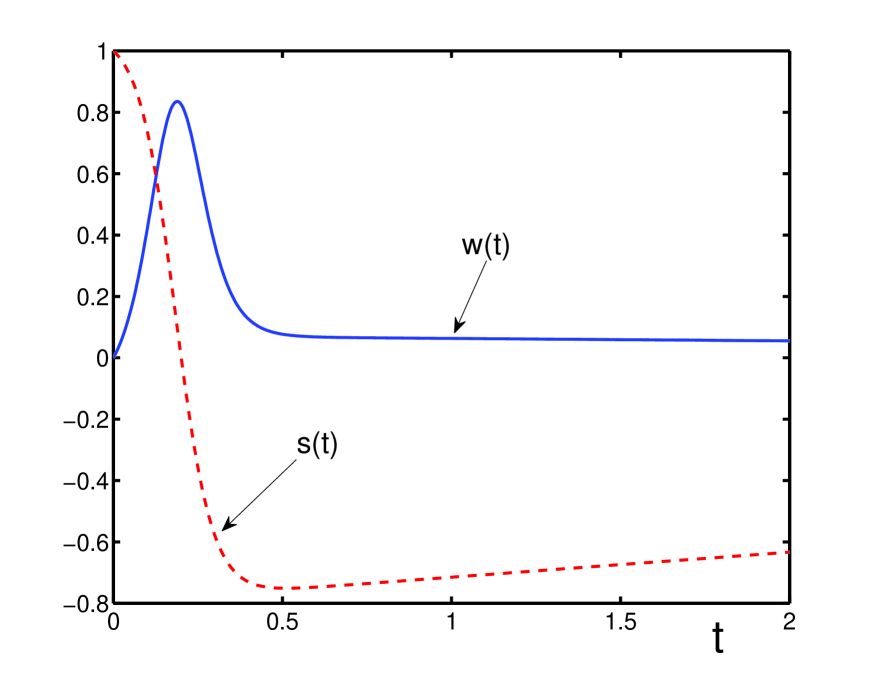
Figure 1: The coherence intensity $w$ (solid line) and population difference $s$ (dashed line) as functions of dimensionless time (measured in units of $T_{2}$) for the attenuation parameters $\gamma_{1}=0.003,\gamma_{3}=1$ (measured in units of $\gamma_{2})$, for the coupling parameter $g=10$, with the initial conditions $w_{0}=0,s_{0}=1$.

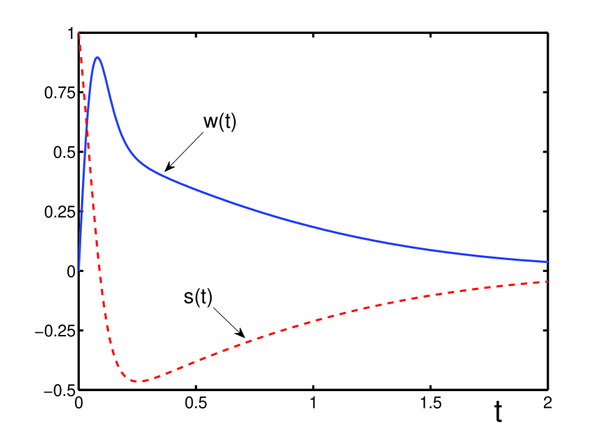
Figure 2: The coherence intensity $w$ (solid line) and population difference $s$ (dashed line) as functions of dimensionless time (measured in units of $T_{2}$) for the attenuation parameters $\gamma_{1}=0.003,\gamma_{3}=10$ (measured in units of $\gamma_{2})$, for the coupling parameter $g=10$, with the initial conditions $w_{0}=0,s_{0}=1$. The larger dynamic attenuation $\gamma_{3}$ makes the pulse more asymmetric.

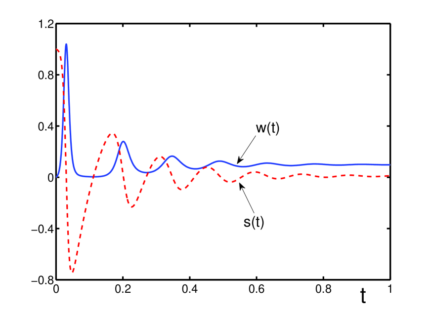
Figure 3: The coherence intensity $w$ (solid line) and population difference $s$ (dashed line) as functions of dimensionless time (measured in units of $T_{2}$) in the case of an external pumping, for the parameters $\gamma_{1}=10,\gamma_{3}=1$ (measured in units of $\gamma_{2})$, for the coupling parameter $g=100$, with the initial conditions $w_{0}=0,s_{0}=1$. The coherence intensity, as well as population difference, exhibit five pulses with decaying amplitude.

Figures 1, 2, and 3 show the evolution of $w=w(t)$ and $s=s(t)$ as functions of dimensionless time $t$, measured in units of $T_{2}\equiv 1/\gamma_{2}$, for several typical cases. We assume that at the initial time, the system is inverted, but coherence is absent and develops in a self-organized way. Recall that the standard mean-field, or semiclassical, approximation cannot describe such a self-organized appearance of coherence. Figures 1 and 2 correspond to the case of no external pumping, when $\zeta=-1$. The difference between these figures is in the value of the dynamical attenuation rate. As we see, the larger $\gamma_{3}$ decreases the delay time and makes the superradiant pulse strongly asymmetric. Recall that for atoms in free space, $\gamma_{3}$ is usually much smaller than $\gamma_{2}$, because of which superradiant pulses produced by atoms are more symmetric. The essential asymmetry of superradiant pulses is the feature typical of quantum-dot radiation. Another typical feature of the quantum-dot dynamics, also caused by the large rate $\gamma_{3}$, is the much faster, than for atoms in free space, tendency of the population difference to the stationary state. Figure 3 demonstrates the radiation dynamics in the case of an external pumping, when $\zeta=1$, and there appear several superradiant pulses with decaying amplitude.

10 Conclusion

The theory of quantum-dot radiation is developed being based on microscopic equations. The possibility of realizing the superradiant regime is analyzed. The temporal evolution during all radiation stages is studied in detail. A special attention is payed to the process when coherence arises from an initially incoherent state. The description of this process is impossible by means of the standard semiclassical equations, because of which a more accurate method has been used in the paper, employing the stochastic mean-field approximation that has been developed earlier and applied for describing the dynamics of spin assemblies [5-11], Bose systems in random fields [38-40], and atomic squeezing [50].

It is necessary to emphasize that the radiation dynamics of quantum dots has several specific features distinguishing this dynamics from atomic radiation. This is connected, first of all, with rather different values of physical dot parameters, as compared to atomic parameters. Because of this, despite many analogies, the theory of dot radiation requires a separate investigation. The principal theoretical points that have been suggested in the present paper for the adequate description of dot radiation are as follows.

(i) Because of essential current fluctuations in semiconductor, the standard semiclassical approximation, often used for atoms in free space, is not applicable for quantum dots. For the latter more elaborate techniques are required, such as the stochastic mean-field approximation.

(ii) Taking into account the fluctuation of current makes the dynamic attenuation parameter $\gamma_{3}$ of the order or larger than $\gamma_{2}$. This is contrary to the case of atoms in free space, where usually $\gamma_{2}$ is the largest relaxation parameter.

(iii) For the correct description and principal understanding of the mechanism, triggering the beginning of the radiation process, it is important to stress the existence of triggering dipolar waves.

(iv) The single-mode picture is not applicable for quantum dots. It is necessary to consider a bunch of transverse modes forming spatial filaments. To reduce the consideration to a treatable problem, it is necessary to involve some tricks, like the transverse-mode expansion.

(v) The overall dynamics of dot radiation consists of several stages, which have been thoroughly studied and described, both analytically and numerically, for the parameters typical of quantum dots.

In the dynamics of dot radiation, it is possible to distinguish the following qualitatively different stages. The first is the fluctuating stage lasting during the time interval $0<t<t_{int}$, when the radiation process is triggered by dipolar waves. At this stage, there is no yet sufficiently strong interaction between dots. The interaction time is of order $t_{int}\sim 10^{-15}s-10^{-14}s$.

The second is the quantum stage in the temporal interval $t_{int}<t<t_{coh}$, when the dot interactions through photon exchange start playing noticeable role, but coherence has not yet been developed. The coherence time, required for the appearance of well developed coherence, is of order $t_{coh}\sim 10^{-14}s-10^{-13}s$.

Then the coherent stage comes into play in the interval $t_{coh}<t<T_{2}$, when the dots emit a coherent superradiant pulse. For the quantum dot materials, the dephasing time is of order $T_{2}\sim 10^{-13}s-10^{-12}s$. The maximum of the pulse occurs at the delay time $t_{0}\simeq 5t_{coh}$ and the pulse duration is $\tau_{p}\simeq 2t_{coh}$. The pulse duration is inversely proportional to the dot density, that is, inversely proportional to the number of dots, involved in the process of radiation, which is a typical feature of superradiance.

After the superradiant pulse is emitted, the system relaxes to an incoherent state during the relaxation stage in the interval $T_{2}<t\ll T_{1}$. The population difference reverses. For the system of dots in a semiconducting material, the longitudinal relaxation time is $T_{1}\sim 10^{-9}s$. But this is not yet the final stage of evolution.

The stationary stage is reached for $t\gtrsim T_{1}$, if there is no external permanent pumping or the effective dot interactions are weak, so that $|g\zeta|\ll 1$. Then the system tends to a stationary incoherent state representing a stable node.

If the system of dots is subject to a sufficiently strong external permanent pumping, such that $|g\zeta|\gg 1$, the regime of pulsing superradiance occurs. Then a series of about 10 superradiant bursts can appear, flashing in the intervals of time $T_{eff}\sim 10^{-13}s$.

Acknowledgement

Financial support from the Russian Foundation for Basic Research is appreciated.

Appendix

Here, the explanation is given of the contributions coming from the dot self-action. For a dot located at $\bf r=0$, the self-action vector potential is

$$A_{self}^{\alpha}({\bf r},t)=\frac{1}{c}\sum_{\beta}\int\frac{\delta_{\alpha\beta}({\bf r}^{\prime})}{|{\bf r}-{\bf r}^{\prime}|}\;J^{\beta}\left(t-\;\frac{|{\bf r}-{\bf r}^{\prime}|}{c}\right)\;d{\bf r}^{\prime}\;,\hskip 113.81102pt(A1)$$

with the current

$${\bf J}\left(t-\;\frac{r}{c}\right)=i\omega_{0}\left[{\bf d}S^{+}(t)e^{-ik_{0}r}-{\bf d}^{*}S^{-}(t)e^{ik_{0}r}\right]\Theta(ct-r)\;,\qquad\quad\qquad\qquad\qquad(A2)$$

in which $S^{\alpha}(t)\equiv S^{\alpha}(0,t)$. At short distance, such that $k_{0}r\ll 1$, one has $\exp(ik_{0}r)\simeq 1+ik_{0}r$. Substituting the transverse delta-function (9) into the vector potential (A1), we keep in mind that the averaging of the dipolar tensor over spherical angles yields zero. As a result, the vector potential (A1) becomes

$${\bf A}_{self}({\bf r},t)=\frac{2}{3}\;k_{0}^{2}\left[{\bf d}S^{+}(t)+{\bf d}^{*}S^{-}(t)\right]+i\;\frac{2k_{0}}{3r}\left[{\bf d}S^{+}(t)-{\bf d}^{*}S^{-}(t)\right]\;.\hskip 56.9055pt(A3)$$

Averaging this expression over the radial variable between the electron wavelength $\lambda_{e}=2\pi/mc$, with $m$ being the electron mass, and the radiation wavelength $\lambda=2\pi/k_{0}$, and taking into account that $\lambda_{e}\ll\lambda$, we get the self-action potential

$${\bf A}_{self}(t)=\frac{2}{3}\;k_{0}^{2}\left[{\bf d}S^{+}(t)+{\bf d}^{*}S^{-}(t)\right]+\frac{ik_{0}}{3\pi}\;\ln\left(\frac{mc^{2}}{\omega_{0}}\right)\left[{\bf d}S^{+}(t)-{\bf d}^{*}S^{-}(t)\right].\hskip 28.45274pt(A4)$$

Let us introduce the natural width

$$\gamma_{0}\equiv\frac{2}{3}\;|{\bf d}|^{2}k_{0}^{2}\hskip 341.43306pt(A5)$$

and the Lamb shift

$$\delta_{L}\equiv\frac{\gamma_{0}}{2\pi}\;\ln\left(\frac{mc^{2}}{\omega_{0}}\right)\;.\hskip 298.75394pt(A6)$$

Then the terms in Eqs. (14), induced by the self-action potential (A4), are

$$2k_{0}S^{z}{\bf d}\cdot{\bf A}_{self}=(i\delta_{L}-\gamma_{2})S^{-}+\frac{{\bf d}^{2}}{|{\bf d}|^{2}}\;(\gamma_{2}+i\delta_{L})S^{+}\hskip 147.95424pt(A7)$$

for the first of Eqs. (14) and

$$k_{0}\left(S_{i}^{+}{\bf d}+S_{i}^{-}{\bf d}^{*}\right)\cdot{\bf A}_{self}=\gamma_{1}\left(\frac{1}{2}+S^{z}\right)\hskip 202.01474pt(A8)$$

for the second, where $\gamma_{1}=2\gamma_{0}$ and $\gamma_{2}=\gamma_{0}$. In the standard situation, one has

$$\frac{\gamma_{0}}{\omega_{0}}\ll 1\;,\qquad\frac{\delta_{L}}{\omega_{0}}\ll 1\;.\hskip 290.21802pt(A9)$$

The Lamd shift, without the loss of generality, can be included in the definition of the transition frequency $\omega_{0}$.

Figure Captions

Fig. 1. The coherence intensity $w$ (solid line) and population difference $s$ (dashed line) as functions of dimensionless time (measured in units of $T_{2}$) for the attenuation parameters $\gamma_{1}=0.003,\gamma_{3}=1$ (measured in units of $\gamma_{2})$, for the coupling parameter $g=10$, with the initial conditions $w_{0}=0,s_{0}=1$.

Fig. 2. The coherence intensity $w$ (solid line) and population difference $s$ (dashed line) as functions of dimensionless time (measured in units of $T_{2}$) for the attenuation parameters $\gamma_{1}=0.003,\gamma_{3}=10$ (measured in units of $\gamma_{2})$, for the coupling parameter $g=10$, with the initial conditions $w_{0}=0,s_{0}=1$. The larger dynamic attenuation $\gamma_{3}$ makes the pulse more asymmetric.

Fig. 3. The coherence intensity $w$ (solid line) and population difference $s$ (dashed line) as functions of dimensionless time (measured in units of $T_{2}$) in the case of an external pumping, for the parameters $\gamma_{1}=10,\gamma_{3}=1$ (measured in units of $\gamma_{2})$, for the coupling parameter $g=100$, with the initial conditions $w_{0}=0,s_{0}=1$. The coherence intensity, as well as population difference, exhibit five pulses with decaying amplitude.

References

- [1] L. Allen and J.H. Eberly, Optical Resonance and Two-Level Atoms (Wiley, New York, 1975).
- [2] A.V. Andreev, V.I. Emelyanov, and Y.A. Ilinsky, Cooperative Effects in Optics (Institute of Physics, Bristol, 1993).
- [3] L. Mandel and E. Wolf, Optical Coherence and Quantum Optics (Cambridge University, Cambridge, 1995).
- [4] M.E. Taşgun, M.Ö. Oktel, L. You, and Ö.E. Müstecaplioğlu, Phys. Rev. A 79, 053603 (2009).
- [5] V.I. Yukalov, Phys. Rev. Lett. 75, 3000 (1995).
- [6] V.I. Yukalov, Laser Phys. 5, 970 (1995).
- [7] V.I. Yukalov, Phys. Rev. B 53, 9232 (1996).
- [8] V.I. Yukalov and E.P. Yukalova, Phys. Part. Nucl. 31, 561 (2000).
- [9] V.I. Yukalov, Laser Phys. 12, 1089 (2002).
- [10] V.I.Yukalov and E.P. Yukalova, Phys. Part. Nucl. 35, 348 (2004).
- [11] V.I. Yukalov, Phys. Rev. B 71, 184432 (2005).
- [12] V.I. Yukalov, V.K. Henner, and P.V. Kharebov, Phys. Rev. B 77, 134427 (2008).
- [13] M. Singh, V.I. Yukalov, and W. Lau, in Nanostructures: Physics and Technology, edited by Z. Alferov and L. Esaki (Ioffe Institute, St. Petersburg, 1998), p. 327.
- [14] Y.N. Chen, D.S. Chuu, and T. Brandes, Phys. Rev. Lett. 90, 166802 (2003).
- [15] V.V. Temnov and U. Woggon, Phys. Rev. Lett. 95, 243602 (2005).
- [16] G. Parascandolo and V. Savona, Phys. Rev. B 71, 045335 (2005).
- [17] A. Sitek and P. Machnikowski, arXiv:0901.0879 (2009).
- [18] M. Scheibner, T. Schmidt, L. Worschech, A. Forchel, G. Bacher, T. Passow, and D. Hommel, Nature Phys. 3, 106 (2007).
- [19] L.P. Kouwenhoven, D.G. Austing, and S. Tarusha, Rep. Prog. Phys. 64, 701 (2001).
- [20] S.M. Reimann and M. Mannien, Rev. Mod. Phys. 74, 1283 (2002).
- [21] 21. C. Yannouleas and U. Landman, Rep. Prog. Phys. 70, 2067 (2007).
- [22] R.G. Nazmitdinov, Phys. Part. Nucl. 40, 71 (2009).
- [23] Y. Arakawa and H. Sakaki, Appl. Phys. Lett. 40, 939 (1982).
- [24] D.L. Huffaker, G. Park, Z. Zou, O.B. Shchekin, and D.G. Deppe, Appl. Phys. Lett. 73, 2564 (1998).
- [25] G. Park, O.B. Shchekin, D.L. Huffaker, and D.G. Deppe, IEEE Photon. Technol. Lett. 12, 230 (2000).
- [26] Y.M. Manz and O.G. Schmidt, Mat. Res. Soc. Symp. Proc. 722, 1141 (2002).
- [27] L.V. Asryan and S. Luryi, Solid-Sate Electron. 47, 205 (2003).
- [28] S. Mokkapati, H.H. Tan, and C. Jagadish, IEEE Photon. Technol. Lett. 18, 1648 (2006).
- [29] J. Liu, Z. Lu, S. Raymond, P.J. Poole, P.J. Barrios, and D. Poitras, Opt. Lett. 33, 1702 (2008).
- [30] B.B. Bakir, C. Seassal, X. Letartre, P. Regreny, M. Gendry, and P. Viktorovitch, Opt. Express 14, 9269 (2006).
- [31] M. Nomura, S. Iwamoto, K. Watanabe, N. Kumagai, Y. Nakata, S. Ishida, and Y. Arakawa, Opt. Express 14, 6308 (2006).
- [32] K. Nozaki, S. Kita, and T. Baba, Opt. Express 15, 7506 (2007).
- [33] M. Nomura, S. Iwamoto, N. Kumagai, and Y. Arakawa, Phys. Rev. B 75, 195313 (2007).
- [34] R. Jodoin and L. Mandel, Phys. Rev. A 9, 873 (1974).
- [35] T.V. Shahbazyan, M.E. Raikh, and Z.V. Vardeny, Phys. Rev. B 61, 13266 (2000).
- [36] R.H. Dicke, Phys. Rev. 93, 99 (1954).
- [37] R. Friedberg, S.R. Hartmann, and J.T. Manassah, Phys. Rep. 7, 101 (1973).
- [38] V.I. Yukalov and R. Graham, Phys. Rev. A 75, 023619 (2007).
- [39] V.I. Yukalov, E.P. Yukalova, K.V. Krutitsky, and R. Graham, Phys. Rev. A 76, 053623 (2007).
- [40] V.I. Yukalov, E.P. Yukalova, and V.S. Bagnato, Laser Phys. 19, 686 (2009).
- [41] A. Keren, O. Shafir, E. Shimshoni, V. Marvaud, A. Bachschmidt, and J. Long, Phys. Rev. Lett. 98, 257204 (2007).
- [42] O. Shafir and A. Keren, Phys. Rev. B 79, 180404 (2009).
- [43] V.I. Yukalov, Laser Phys. 3, 870 (1993).
- [44] V.I. Yukalov and E.P. Yukalova, Laser Phys. Lett. 2, 302 (2005).
- [45] V.I. Yukalov, Laser Phys. Lett. 2, 356 (2005).
- [46] V.I. Yukalov, Laser Phys. 19, 1 (2009).
- [47] C.J. Joachain, Quantum Collision Theory (North-Holland, Amsterdam, 1975).
- [48] R.G. Newton, Scattering Theory of Waves and Particles (Springer, New York, 1982).
- [49] N.N. Bogolubov and Y.A. Mitropolsky, Asymptotic Methods in the Theory of Nonlnear Equations (Gordon and Breach, New York, 1961).
- [50] V.I. Yukalov and E.P. Yukalova, Phys. Rev. A 70, 053828 (2004).