Thermal Breakage and Self-Healing of a Polymer Chain under Tensile Stress

Abstract

We consider the thermal breakage of a tethered polymer chain of discrete segments coupled by Morse potentials under constant tensile stress. The chain dynamics at the onset of fracture is studied analytically by Kramers-Langer multidimensional theory and by extensive Molecular Dynamics simulations in $1D$- and $3D$-space. Comparison with simulation data in one- and three dimensions demonstrates that the Kramers-Langer theory provides good qualitative description of the process of bond-scission as caused by a collective unstable mode. We derive distributions of the probability for scission over the successive bonds along the chain which reveal the influence of chain ends on rupture in good agreement with theory. The breakage time distribution of an individual bond is found to follow an exponential law as predicted by theory. Special attention is focused on the recombination (self-healing) of broken bonds. Theoretically derived expressions for the recombination time and distance distributions comply with MD observations and indicate that the energy barrier position crossing is not a good criterion for true rupture. It is shown that the fraction of self-healing bonds increases with rising temperature and friction.

I Introduction

A great variety of problems both in material and basic science rely on the fundamental understanding of the intramolecular dynamics and kinetics of fragmentation (bond rupture) of linear macromolecular subject to a tensile force. Typical examples comprise material failure under stress Kausch ; Crist , polymer rupture Garnier ; Gaub ; Saitta ; Maroja ; Rohrig , adhesion Gersappe , friction Klafter , mechanochemistry Aktah ; Beyer , and biological applications of dynamical force microscopy Harris ; Pereverzev . In particular, the problem of polymer rupture as a kinetic process has a longstanding history and dates back to the publications of Bueche Bueche and Zhurkov et al. Zhurkov . In these papers the breaking of intramolecular bonds is treated as a thermally activated process and is described by Arrhenius’s formula for the rate of bond scission.

In recent years investigations have been complemented by ample application of computer experiments. Comprehensive Molecular Dynamic (MD) simulations of $1D$ chain fragmentation (at constant strain) have been carried out, whereby harmonic Taylor ; Lee , Morse Stember ; Bolton ; Sebastian , or Lennard-Jones Oliveira_1 ; Oliveira_2 ; Oliveira_3 ; Oliveira_4 chain models have been used. One of the principal questions to be answered is : “How long will it take for this system to break?”. A theoretical interpretation of MD-results Oliveira_3 ; Oliveira_4 , based on an effectively one-particle model, has been suggested in terms of Kramers rate theory Kramers . Thus, the activation energy of the one-particle model $E_{b}$ has been found to be close to the barrier height observed in the simulations, whereas the measured frequency of bond scission appears more than two orders of magnitudes smaller then the corresponding frequency, predicted by Kramers theory. The authors interpret this controversial result as a manifestation of the existence of collective modes which are missing in the one-particle Kramers theory.

It has also been noticed that a truly irreversible break may occur, if bonds are stretched to lengths, considerably larger than the one corresponding to the barrier position. This indicates the possibility for bond recombination whereby the chain integrity is restored with some finite probability.

The problem of polymer fragmentation has also been studied theoretically Sebastian for the case of constant stress when a tethered chain of segments is subjected to a pulling force at the free chain end. The consideration has been based on a multidimensional version of the transition state theory (TST). Friction is then taken into account by coupling the polymer to a set of harmonic oscillators, simulating thus the presence of a thermostat. A comparison of the calculated breaking rate with the corresponding MD observation Oliveira_1 shows again that the theoretical rate is about 250 times larger. Also the role of the bond healing process has been discussed which helps to improve to some extent the agreement between theory and simulation. Nevertheless, despite the multidimensional nature of TST, it does not take into account properly the collective unstable mode development, which leads, in our opinion, to the essential overestimation of the breaking rate.

The collectivity effect has been recently treated Sain for constant strain and periodic boundary conditions (a ring polymer) on the basis of the multidimensional Kramers approach Langer ; Hanngi . Within this approach the development of a collective unstable mode and the effect of dissipation can be described consistently. It has been shown that in this case the effective break frequency is of the same order of magnitude as the one observed in the simulation.

In the present work we develop this approach further for the case of a tethered Morse chain, consisting of $N$ segments and subjected to a constant tensile force $f$ applied at its free end. We derive analytic expressions for the scission rate of the bonds, its distribution along the polymer chain, and its variation with changing temperature and dissipation. For comparison with computer experiment, we also perform extensive MD simulations in both one- $1D$, and three dimensions, $3D$, and witness significant differences in the fragmentation behavior of the chain, despite the observed good agreement between theoretical predictions and simulation data. A major objective of the current study is the elucidation of the problem of bond recombination (self-healing) which has found little attention in literature so far. To this end we derive analytic expressions for the life times and extension distances of healing bonds and compare them to our MD results.

The paper is organized as follows. In Section II we give a sketch of the multidimensional Kramers-Langer escape theory Langer ; Hanngi . We also outline the problem of multiple points of exit from potential well Matkowsky ; Gardiner which is necessary for treating bond rupture with respect to the consecutive number of each bond along the chain. In Section III we present our model of one-dimensional Morse string of beads and consider the eigenvalue problem in the vicinity of the metastable minimum of the effective potential and at the barrier (saddle point) which is needed for the description of the unstable collective mode. Section IV gives briefly details of our MD simulation and presents the main numeric results as well as their interpretation in the light of our theoretical approach. In Section V the healing process is discussed in terms of distributions of healing times and bond extensions. We give also the theoretical interpretation of this process based on the solution of the Kramers equation Risken using an inverted harmonic potential for representation of the barrier. We conclude in Section VI and outline some future developments.

II Kramers-Langer multidimensional escape theory

II.1 Rate of escape

The calculation of the rate of escape is based on the $N$-dimensional (in the total phase space $x_{i}=q_{i}$, $x_{i+N}=p_{i}$, $i\leq N$ Goldstein ) Fokker-Planck equation Risken

$$\dfrac{\partial P({\bf x},t)}{\partial t}=\sum_{i,j=1}^{2N}\>\dfrac{\partial}{\partial x_{i}}\>M_{ij}\left[\dfrac{\partial H}{\partial x_{j}}\>P({\bf x},t)+T\dfrac{\partial}{\partial x_{j}}\>P({\bf x},t)\right]$$ (1)

for the probability distribution function $P({\bf x},t)\equiv P(\{x_{i}\},t)$. In eq. (1) the Hamiltonian has a general form $\sum_{i=1}^{N}\>p_{i}^{2}/2m+V(\{q_{i}\})$. The $2N\times 2N$-matrix $M_{ij}=\Gamma_{ij}-A_{ij}$ , where $\Gamma_{ij}$ is the matrix of Onsager coefficients and $2N\times 2N$ skew-symmetric matrix Goldstein

$$\overrightarrow{A}=\left(\begin{array}[]{ccc}\overrightarrow{0}&\overrightarrow{1}\\ -\overrightarrow{1}&\overrightarrow{0}\end{array}\right)$$ (4)

where $\overrightarrow{1}$ is the $N\times N$ unit matrix and $\overrightarrow{0}$ is the $N\times N$ zero matrix. The eq.(1) can be seen as a continuity equation, $\partial P/\partial t=-\sum_{i=1}^{2N}\>\partial/\partial x_{i}\>J_{i}$, where the probability current is given by $J_{i}=-\sum_{j=1}^{2N}M_{ij}\left(\partial H/\partial x_{j}P({\bf x},t)+T\partial P({\bf x},t)/\partial x_{j}\right)$.

It is assumed Langer that there is a metastable state $\{x_{i}^{A}\}$ which is separated with a barrier from another stable state. The coordinates at the saddle point which separates these two states is denoted by $\{x_{i}^{S}\}$. The escape from the metastable minima is a comparatively rare event, so that one can treat the process close to $\{x_{i}^{S}\}$ as a stationary one, i.e. $\sum_{j=1}^{2N}\partial J_{j}/\partial x_{j}=0$. Thus one gets

$$\sum_{i,j=1}^{2N}\>\dfrac{\partial}{\partial x_{i}}\>M_{ij}\>\left[\sum_{k}{\rm E}_{jk}^{S}(x_{k}-x_{k}^{S})+T\dfrac{\partial}{\partial x_{j}}\>\right]P({\bf x})=0$$ (5)

where also the harmonic approximation around $\{x_{i}^{S}\}$ has been used, i.e., the Hamiltonian reads

$$H(\{x_{i}\})=E^{S}+\dfrac{1}{2}\sum_{j,k=1}^{2N}{\rm E}_{jk}^{S}(x_{j}-x_{j}^{S})(x_{k}-x_{k}^{S})$$ (6)

where $E^{S}=H(\{x_{i}^{S}\})$ and the Hessian matrix $E_{ij}^{S}=\partial^{2}H/\partial x_{i}\partial x_{j}$ at $\{x_{i}\}=\{x_{i}^{S}\}$.

One should impose the following boundary conditions. Near the metastable state $\{x_{i}^{A}\}$ the distribution function $P({\bf x})$ is the equilibrium one, i.e.

$$P({\bf x})=P_{\rm eq}({\bf x})=Z_{A}^{-1}\>\exp(-\beta H)\qquad\mbox{at}\qquad{\bf x}\simeq\{x_{i}^{A}\}$$ (7)

On the other hand, all states around the stable minimum (which is far beyond the top of the barrier!) are removed by a sink, i.e.,

$$P({\bf x})\simeq 0\qquad\mbox{at}\quad\{x_{i}\}\quad\mbox{far beyond}\quad\{x_{i}^{S}\}$$ (8)

With a transformation to new coordinates $\xi_{n}=\sum_{i=1}^{2N}D_{ni}(x_{i}-x_{i}^{S})$, which are principal-axis coordinates for the Hamiltonian given by eq.(6), one obtains

$$H({\bm{\xi}})=E^{S}+\dfrac{1}{2}\>\sum_{n=1}^{2N}\>\lambda_{n}\>\xi_{n}^{2}+\dots$$ (9)

where the vector ${\bm{\xi}}\equiv\{\xi_{n}\}$. The matrix $D_{ni}$ is orthogonal one, i.e. $D^{T}=D^{-1}$ and $\{\lambda_{n}\}$ are the eigenvalues of the matrix ${\rm E}_{ij}^{S}$. Since $\{x_{i}^{S}\}$ is a saddle point one of the $\lambda$’s, say $\lambda_{1}$, is negative. The standard trick would be to look for the solution in the form $P({\bm{\xi}})=W({\bm{\xi}})P_{\rm eq}({\bm{\xi}})$ , where $W({\bm{\xi}})$ is a new function. Thus in the $\xi$-coordinate system the steady - state Fokker Planck equation for $W({\bm{\xi}})$ takes the form

$$\sum_{n,k=1}^{2N}\>\left({\widetilde{\Gamma}}_{nk}\>\dfrac{\partial^{2}W}{\partial\xi_{n}\partial\xi_{k}}-\beta\lambda_{n}\xi_{n}\>{\widetilde{M}}_{nk}\dfrac{\partial W}{\partial\xi_{k}}\right)=0$$ (10)

where ${\widetilde{M}}_{nk}=\sum_{i,j}\>D_{ni}M_{ij}D_{kj}={\widetilde{\Gamma}}_{nk}-{\widetilde{A}}_{nk}$.

In the same manner as for the one-dimensional Kramers problem Kramers one could claim that the function $W({\bm{\xi}})$ depends only on a linear combination of all $\xi_{n}$, i.e. $W(\{\xi_{k}\})=F(u)$, where $u=\mathop{{\sum}^{\prime}}_{n}\>U_{n}\>\xi_{n}$ . The prime in this expression indicates that we omit all $n$’s for which $\lambda_{n}=0$. The resulting equation reads: $\sum_{n,k}\left[({\widetilde{\Gamma}}_{nk}\>U_{n}\;U_{k})\>d^{2}F/du^{2}-\beta(\lambda_{n}\>\xi_{n}{\widetilde{M}}_{nk}\>U_{k})dF/du\right]=0$. As in the one-dimensional Kramers problem Kramers the coefficient in front of $dF/du$ is a linear function of $u$, i.e. $\sum_{n,k}\lambda_{n}\>\xi_{n}{\widetilde{M}}_{nk}\>U_{k})=\kappa u=\kappa\mathop{{\sum}^{\prime}}_{n}\>U_{n}\>\xi_{n}$. As a result

$$\lambda_{n}\>\sum_{k}{\widetilde{M}}_{nk}\>U_{k}=\kappa\>U_{n}$$ (11)

i.e., the coefficients $U_{n}$ are solutions of the eigenvalue problem eq. (11). Thus,

$$T\>\lambda_{+}\>\dfrac{d^{2}F(u)}{du^{2}}-u\dfrac{dF(u)}{du}=0$$ (12)

where

$$\lambda_{+}=\dfrac{1}{\kappa}\>\sum_{n,k}\>U_{n}\>{\widetilde{\Gamma}}_{nk}\>U_{k}$$ (13)

There is a simple physical interpretation of the eigenvalue problem given by eq. (11) Langer . Namely, the equation of motion for the average value, $\left\langle\xi_{n}(t)\right\rangle=\int\prod_{j=1}^{2N}\xi_{n}P(\{\xi_{j}\},t)$ can be written as

$$\dfrac{\partial}{\partial t}\left\langle\xi_{n}(t)\right\rangle=\int\prod_{j=1}^{2N}\>d\xi_{j}\>\widetilde{J}(\{\xi\},t)=-\dfrac{T}{Z_{A}}\sum_{k}\>{\widetilde{M}}_{nk}\>\int\prod_{j=1}^{2N}\>d\xi_{j}\>\dfrac{\partial W}{\partial\xi_{k}}\>{\rm e}^{-\beta H}$$ (14)

With integration by parts and the harmonic approximation, eq. (9), one arrives at the following expression

$$\dfrac{\partial}{\partial t}\left\langle\xi_{n}(t)\right\rangle=-\sum_{k}\>{\widetilde{M}}_{nk}\>\lambda_{k}\>\left\langle\xi_{k}(t)\right\rangle$$ (15)

The unstable solution of this equation (which describes the decay of a metastable state) is given by a negative eigenvalue $\kappa$, namely

$$\left\langle\xi_{n}(t)\right\rangle=X_{n}\>{\rm e}^{-\kappa t}$$ (16)

Substitution of eq.(16) in eq. (15) leads to $\sum_{k}\>{\widetilde{M}}_{nk}\>\lambda_{k}\>X_{k}=\kappa X_{n}$ or

$$\lambda_{n}\>\sum_{k}{\widetilde{M}}_{nk}\>\lambda_{k}\>X_{k}=\kappa\lambda_{n}X_{n}$$ (17)

This equation is identical to eigenvalue problem, eq. (11), provided that $U_{n}=\lambda_{n}X_{n}$. There is a negative eigenvalue $\kappa$ and as a result a negative $\lambda_{+}$ (see eq.(13)) which corresponds to the unstable mode. This clear physical interpretation justifies the linear combination ansatz which has been used upon the derivation of eq. (12). We will show in Sec. IV devoted to MD-simulation results that the law given by eq. (16) actually holds for the breaking bonds.

With the negative eigenvalue, $\lambda_{+}<0$, the solution of eq.(12) takes the form

$$F(u)=\dfrac{1}{\sqrt{2\pi|\lambda_{+}|T}}\>\int_{u}^{\infty}\>dz\>\exp\left(-\dfrac{z^{2}}{2|\lambda_{+}|T}\right)$$ (18)

In eq.(18) we take into account the boundary conditions, eqs.(7) and (8) which require $F(u\rightarrow-\infty)=1$ (at the metastable well) and $F(u\rightarrow\infty)=0$ (around the stable minimum).

Consider the rate of the metastable state decay. The main quantity which should be used for this purpose is the the probability current

$${\widetilde{J}}_{n}=-\dfrac{T}{Z_{A}}\>\sum_{k}{\widetilde{M}}_{nk}\>U_{k}\>\dfrac{dF(u)}{du}\>{\rm e}^{-\beta H}$$ (19)

To obtain the total probability flux over the barrier one should integrate the current, eq. (19), over the hypersurface $u=\mathop{\sum^{\prime}}_{n}U_{n}\xi_{n}=0$ containing the saddle point. The resulting flux reads

$$J=\int\prod_{i=1}^{2N}\>d\xi_{i}\>\delta(u)\>\sum_{n=1}^{2N}\>U_{n}{\widetilde{J}}_{n}(\{\xi_{i}\})$$ (20)

The calculation of this integral is given in Appendix of ref. Hanngi . The calculation yields

$$J=\dfrac{|\kappa|}{2\pi}\>\left(\dfrac{2\pi T}{|\lambda_{1}|}\right)^{1/2}\>\prod_{n=2}^{2N}\left(\dfrac{2\pi T}{\lambda_{n}}\right)^{1/2}\>\dfrac{{\rm e}^{-\beta E^{S}}}{Z_{A}}$$ (21)

In order to obtain the rate constant one must divide the flux over the popularion $n_{A}$ in the metastable well

$$n_{A}=\int\limits_{A_{well}}\>\prod_{i=1}^{2N}\>d\xi_{i}P_{\rm eq}(\{\xi_{i}\})=\dfrac{{\rm e}^{-\beta E^{A}}}{Z_{A}}\>\prod_{i=1}^{2N}\>\left(\dfrac{2\pi T}{\lambda_{n}^{a}}\right)^{1/2}$$ (22)

where we have used the harmonic approximation near the metastable state $\{x_{i}^{A}\}$, i.e. $H=E^{A}+\sum_{n=1}^{2N}\lambda_{n}^{a}\xi_{n}^{2}/2$. Combining eq.(21) and eq.(22), one finds for the rate constant, $k=J/n_{A}$, the following result Langer

$$k=\dfrac{|\kappa|}{2\pi}\>\>\left[\dfrac{{\rm det}({\bf E}^{A}/2\pi T)}{|{\rm det}({\bf E}^{S}/2\pi T)|}\right]^{1/2}\>{\rm e}^{-\beta E_{b}}$$ (23)

where the activation barrier $E_{b}=E^{S}-E^{A}$. We recall that $\lambda_{n}$ are the eigenvalues (without zero-modes) of the Hessian matrix ${\bf E}^{S}$ at the saddle point ${\bf x}^{S}$ whereas $\lambda_{n}^{a}$ are the the eigenvalues of the Hessian matrix ${\bf E}^{A}$ at the metastable point ${\bf x}^{A}$.

II.2 The eigenvalue problem

Consider in more detail the eigenvalue problem given by eq. (17), i.e.$\sum_{k}{\widetilde{M}}_{nk}\>\lambda_{k}\>X_{k}=\kappa X_{n}$. In the initial $x$-space this equation reads

$$\sum_{k,r}M_{nk}\>E_{kr}^{S}\>X_{r}=\kappa X_{n}$$ (24)

where $M_{ij}=\Gamma_{ij}-A_{ij}$ and the friction $\Gamma_{ij}$ as well as the matrix $A_{ij}$ are given as

$$\Gamma_{ij}=m\gamma\left(\begin{array}[]{ccc}\begin{array}[]{ccc}0&\cdots&0\\ \vdots&&\vdots\\ 0&\cdots&0\end{array}&&\begin{array}[]{ccc}0&\cdots&0\\ \vdots&\ddots&\vdots\\ 0&\cdots&0\end{array}\\ \begin{array}[]{ccc}0&\cdots&0\\ \vdots&\ddots&\vdots\\ 0&\cdots&0\end{array}&&\begin{array}[]{ccc}1&\cdots&0\\ \vdots&\ddots&\vdots\\ 0&\cdots&1\end{array}\end{array}\right)\qquad A_{ij}=\left(\begin{array}[]{ccc}\begin{array}[]{ccc}0&\cdots&0\\ \vdots&&\vdots\\ 0&\cdots&0\end{array}&&\begin{array}[]{ccc}1&\cdots&0\\ \vdots&\ddots&\vdots\\ 0&\cdots&1\end{array}\\ \begin{array}[]{rcr}-1&\cdots&0\\ \vdots&\ddots&\vdots\\ 0&\cdots&-1\end{array}&&\begin{array}[]{ccc}0&\cdots&0\\ \vdots&&\vdots\\ 0&\cdots&0\end{array}\end{array}\right)$$ (53)

The $2N\times 2N$ Hessian matrix and the $2N$-dimensional column-vector are

$$E_{ij}^{S}=\left(\begin{array}[]{ccc}\dfrac{\partial^{2}V}{\partial q_{i}\partial q_{j}}&&\begin{array}[]{ccc}0&\cdots&0\\ \vdots&&\vdots\\ 0&\cdots&0\end{array}\\ \begin{array}[]{ccc}0&\cdots&0\\ \vdots&&\vdots\\ 0&\cdots&0\end{array}&&\begin{array}[]{ccc}1/m&\cdots&0\\ \vdots&\ddots&\vdots\\ 0&\cdots&1/m\end{array}\end{array}\right)\qquad X_{i}=\left(\begin{array}[]{c}q_{1}\\ q_{2}\\ \vdots\\ q_{N}\\ p_{1}\\ p_{2}\\ \vdots\\ p_{N}\end{array}\right)$$ (73)

After substitution of eqs. (53) and (73) into eq. (24), and exclusion of momentums $\{p_{i}\}$, one arrives at the eigenvalue problem

$$\sum_{j=1}^{N}\>\underbrace{\left[V_{ij}^{S}-m\gamma\kappa\delta_{ij}\right]}_{\mbox{$N\times N$ - matrix}}\>X_{j}=-m\kappa^{2}X_{i}$$ (74)

where the notation $V_{ij}^{S}=\partial^{2}V/\partial q_{i}\partial q_{j}|_{S}$ is used. The corresponding characteristic equation Lancaster reads

$$\det\left[m\kappa^{2}\delta_{ij}-m\gamma\kappa\delta_{ij}+V_{ij}^{S}\right]=\prod_{k=1}^{N}[m\kappa^{2}-m\gamma\kappa+\lambda_{k}]=0$$ (75)

where $\{\lambda_{k}\}$ is a set of eigenvalues of the Hessian $V_{ij}^{S}$. As mentioned before, only one eigenfunction, say $\lambda_{1}$, is negative. This eigenvalue determines then the equation for the transmission factor $\kappa$, i.e.

$$\kappa^{2}-\gamma\kappa-\dfrac{|\lambda_{1}|}{m}=0$$ (76)

The negative solution reads

$$\kappa=-\sqrt{\dfrac{\gamma^{2}}{4}+\dfrac{|\lambda_{1}|}{m}}+\dfrac{\gamma}{4}\><0$$ (77)

Eq. (75) has been discussed first in ref. Weidenmuller .

II.3 First-passage-time approach

The method of Section II.1 is a quite general approach to evaluate the rate of escape from the metastable state. The alternative to the flux-over-population method involves the concept of mean first-passage time. For an arbitrary stochastic multi-dimensional process ${\bf x}(t)$ the mean first-passage time (MFPT) $T_{1}(x)$ is defined as the average time elapsed until the process starting out at point ${\bf x}$ leaves a prescribed domain $\Omega$ which includes the point ${\bf x}^{A}$ of the reactant state. $\Omega$ is sometimes called domain of attraction of the metastable state, and is shown in Fig. 1

Figure 1: Exit from the phase space domain $\Omega$. Vectors denote the restoring force directions. The trajectory starts close to the metastable minimum and exits through a particular exit (saddle) point.

For the FPT investigation it is convenient to use the Fokker-Planck equation (for the conditional probability $P({\bf y},t;{\bf x},0)$ of visiting the point ${\bf y}\in\Omega$ at time $t$, provided it starts from ${\bf x}\in\Omega$ at $t=0$) which includes the so called adjoint operator and has the form Risken

$$\dfrac{\partial}{\partial t}\>P({\bf y},t;{\bf x},0)=L^{\dagger}({\bf x})\>P({\bf y},t;{\bf x},0)$$ (78)

where the adjoint operator

$$L^{\dagger}({\bf x})=\sum_{i}\>K_{i}({x})\>\dfrac{\partial}{\partial x_{i}}\>+\varepsilon\>\sum_{i,j}\>D_{ij}({\bf x})\>\dfrac{\partial^{2}}{\partial x_{i}\partial x_{j}}\>$$ (79)

In the present case the drift and diffusion coefficients are respectively: $K_{i}({\bf y})=-\sum_{j}M_{ij}\partial H/\partial y_{j}$ and $D_{ij}=\Gamma_{ij}$. In eq. (79) $\varepsilon$ is responsible for the noise intensity (in our case $\varepsilon$ plays the role of the temperature), so that at $\varepsilon\rightarrow 0$ the noise is weak.

The $n$-th order moments of the first-passage time, $T_{n}({\bf x})$, may be iteratively expressed in terms of the adjoint operator, Risken

$$L^{\dagger}({\bf x})\>T_{n}({\bf x}) = -nT_{n-1}({\bf x})\quad,\quad\mbox{at}\quad{\bf x}\in\Omega$$

$$T_{n}({\bf x}) = 0\quad,\quad\mbox{at}\quad{\bf x}\in\partial\Omega$$ (80)

where the second equation simply means that the first passage time is zero, provided the trajectory starts at the separatrix $\partial\Omega$. The hierarchy given by eq. (80) should be supplemented by the initial condition $T_{0}({\bf x})=1$ which is evident from the normalization condition for the FPT distribution. Therefore, the equation for the mean first passage time (MFPT), $T_{1}({\bf x})$, reads

$$L^{\dagger}({\bf x})\>T_{1}({\bf x}) = -1\quad,\quad\mbox{at}\quad{\bf x}\in\Omega$$

$$T_{1}({\bf x}) = 0\quad,\quad\mbox{at}\quad{\bf x}\in\partial\Omega$$ (81)

On the other hand, for small noise, $\varepsilon\rightarrow 0$, a trajectory starting within $\Omega$ will typically first approach the attractor and stay within its neighborhood for a long time until an occasional fluctuation drives it to the separatrix $\partial\Omega$. Hence, MFPT $T_{1}({\bf x})$ assumes the same large value $\tau$ everywhere in $\Omega$ except for a thin layer along the boundary $\partial\Omega$. Under these condition the solution of the hierarchical equation, eq.(80), can be obtained in the following form Talkner : $T_{1}=\tau,T_{2}=2\tau^{2},T_{3}=2\cdot 3\tau^{3},\ldots,T_{n}=n!\>\tau^{n}$. In result the probability density of the first passage times reads Talkner

$$p(t)=\tau^{-1}\exp(-t/\tau)$$ (82)

(we recall that $\tau^{-1}\int_{0}^{\infty}t^{n}\exp(-t/\tau)dt=n!\tau^{n}$). The validity of this PDF has been shown in our MD-simulation (see Sec. IV). Finally, it can be proven Talkner ; Hanngi that the Kramers escape rate $k=(2\tau)^{-1}$.

II.4 Distribution of exit points

Assume that there are a number of saddle points, ${\bf b}^{r}$ where $r=1,2,\dots M$, (referred to as exit points)which lie on the separatrix. We study then the exit events (see Fig. 1 where only two exit points are shown). One may ask : “What is the probability to exit through a particular exit point ${\bf b}^{S}\in\partial\Omega$ irrespective of the time it takes?” This problem has been discussed first by Matkowsky and Schuss Matkowsky and later by Gardiner Gardiner . Here we give an explicit solution which may be compared to MD-simulations.

The probability for escape through an exit point ${\bf b}^{S}$ if the random trajectory starts at ${\bf x}\in\Omega$ is defined as

$$\pi({\bf b}^{S};{\bf x})=\int\limits_{0}^{\infty}\>dt^{\prime}\sum\limits_{i}\>\nu_{i}({\bf b}^{S})J_{i}({\bf b}^{S},t^{\prime}|{\bf x},0)$$ (83)

where $\nu_{i}({\bf b}^{S})$ is a component of the vector normal to the separatrix unit vector at ${\bf b}^{S}$ pointing out of region $\Omega$. The flux $J_{i}({\bf b}^{S},t^{\prime}|{\bf x},0)$ counts only trajectories which start at $t=0$ in ${\bf x}\in\Omega$ and approach the exit point ${\bf b}^{S}$ at the boundary (separatrix) at time moment $t^{\prime}$. The integral over time in eq. (83) implies that this probability is calculated irrespective of the time needed for escape.

The probability $\pi({\bf b}^{S};{\bf x})$ is governed by the backward stationary FPE, i.e. (see Sec. 5.4.2 in Gardiner )

$$L^{\dagger}({\bf x})\>\pi({\bf b}^{S};{\bf x})=0$$ (84)

The boundary conditions are: $\pi({\bf b}^{S};{\bf b}^{S})=1$ and $\pi({\bf b}^{S};{\bf x})=0$ for any ${\bf x}\in\partial\Omega$ if ${\bf x}\neq{\bf b}^{S}$, i.e.,

$$\pi({\bf b}^{S};{\bf x})=\delta_{s}({\bf b}^{S}-{\bf x})\qquad\mbox{for}\qquad{\bf x}\in\partial\Omega$$ (85)

Using the same arguments as in Sec. II.3, one can show that in the small noise limit, $\varepsilon\rightarrow 0$, the probability $\pi({\bf b}^{S};{\bf x})$ remains the same everywhere inside $\Omega$ apart from a thin layer along the boundary $\partial\Omega$. Now we specify the general eq. (84) for the special case when the drift term has the form of potential (i.e., it is derivative of the Hamiltonian). Then eq. (84) reads

$$\sum\limits_{i,j}\left[-M_{ij}\dfrac{\partial H}{\partial x_{j}}\>\dfrac{\partial}{\partial x_{i}}+\varepsilon M_{ij}\>\dfrac{\partial^{2}}{\partial x_{i}\partial x_{j}}\right]\pi({\bf b}^{S};{\bf x})=0$$ (86)

Close to the saddle point the Hamiltonian can be treated in the harmonic approximation, eq. (6), and the drift velocity in eq. (86) becomes

$$K_{i}=-\sum\limits_{j}\>M_{ij}\dfrac{\partial H}{\partial x_{j}}=-\sum\limits_{j,k}\>M_{ij}E_{jk}^{S}(x_{k}-b_{k}^{S})$$ (87)

Since the solution changes only within a thin layer along the boundary (in direction normal to the boundary layer!), one may introduce new local coordinates $\{z,y_{p}\}$ where $z$ measures the distance from ${\bf b}^{S}$ and $\{y_{p}\}$ is the set of tangential variables measuring the orientation around ${\bf b}^{S}$. The coordinates $z=z({\bf x})$ and $y_{p}=y_{p}({\bf x})$ are chosen so that

$$\nabla z({\bf u}) = \bm{\nu}({\bf u})$$

$$\bm{\nu}({\bf u})\cdot\nabla y_{p}({\bf u}) = 0$$

$$z({\bf b}^{S}) = 0$$ (88)

where ${\bf u}\in\partial\Omega$. The first equation in (88) means that the coordinate $z$ changes in direction of the $\bm{\nu}$-vector. The second equation implies that the coordinates $\{y_{p}\}$ are parallel to $\partial\Omega$. In terms of new variables

$$\nabla_{i}\pi=\nu_{i}\dfrac{\partial\pi}{\partial z}+\sum\limits_{p}\nabla_{i}y_{p}({\bf x})\dfrac{\partial\pi}{\partial y_{p}}$$ (89)

and

$$\nabla_{i}\nabla_{j}\pi = \nu_{i}\>\nu_{j}\>\dfrac{\partial^{2}\pi}{\partial z^{2}}+2\sum\limits_{p}\nu_{i}\>\nabla_{j}y_{p}({\bf x})\>\dfrac{\partial^{2}\pi}{\partial z\partial y_{p}}+\sum\limits_{p,s}\>\nabla_{i}y_{p}({\bf x})\nabla_{j}y_{s}({\bf x})\>\dfrac{\partial^{2}\pi}{\partial y_{p}\partial y_{r}}$$ (90)

$$+ \nabla_{i}\nabla_{j}z({\bf x})\>\dfrac{\partial\pi}{\partial z}+\sum\limits_{p}\nabla_{i}\nabla_{j}y_{p}({\bf x})\>\dfrac{\partial\pi}{\partial y_{p}}$$

One should keep in mind that for the exit event at $\varepsilon\rightarrow 0$ only one coordinate is relevant, namely, the one traversing the saddle point in direction of $\bm{\nu}$ vector. This is our new $z$-coordinate, which parameterizes the displacement from the saddle point as follows

$$x_{j} = b_{j}^{S}+z\>\nu_{j}$$

$$z = \sqrt{\varepsilon}\rho$$ (91)

Substituting eqs.(89)- (91) in eqs. (86) and (87), and keeping only the lowest order in $\varepsilon$, leads to

$$\lambda_{+}\>\dfrac{\partial^{2}\pi}{\partial\rho^{2}}-\rho\>\dfrac{\partial\pi}{\partial\rho}=0$$ (92)

where

$$\lambda_{+}=\dfrac{1}{\kappa}\>\sum_{i,j}\>\nu_{i}\>\Gamma_{ij}\>\nu_{j}=\dfrac{m\gamma}{\kappa}\;.$$ (93)

In (93)one has used $\sum_{i,j}\>\nu_{i}\>M_{ij}\>\nu_{j}=\sum_{i,j}\>\nu_{i}\>\Gamma_{ij}\>\nu_{j}$ and taken into account $\sum_{i,j}\;\nu_{i}\>\Gamma_{ij}\>\nu_{j}=m\gamma$ (Appendix A) as well as

$$\kappa=\sum\limits_{i,j,k}\>\nu_{i}\>M_{ij}E_{jk}^{S}\>\nu_{k}$$ (94)

The solution of eq.(92) has the form

$$\pi({\bf b}^{S};{\bf u},\rho)=\delta({\bf u}-{\bf b}^{S})+[C_{\infty}-\delta({\bf u}-{\bf b}^{S})]\left(\dfrac{2}{\pi|\lambda_{+}|}\right)^{1/2}\>\int\limits_{0}^{\rho}\>dz\exp\left[-\dfrac{z^{2}}{2|\lambda_{+}|}\right]$$ (95)

where we took into account the boundary condition $\pi({\bf b}^{S};{\bf u},0)=\delta({\bf u}-{\bf b}^{S})$ (vector ${\bf u}\in\partial\Omega$) and at $\rho\rightarrow-\infty$ $\pi({\bf b}^{S})=C_{\infty}$, i.e., well inside the region $\Omega$ the solution is a constant as this should be for a weak noise. In order to fix the constant $C_{\infty}$ one may multiply eq. (86) by $p_{\rm st}({\bf x})$ and after integrating over $\Omega$ (using also the integration by parts and the Gauss theorem) derive the surface integral

$$\int\limits_{\partial\Omega}\>dS\left\{-p_{\rm st}\sum\limits_{i,j}\nu_{i}M_{ij}\nabla_{j}H\>\pi+\varepsilon\left[p_{\rm st}\sum\limits_{i,j}\nu_{i}M_{ij}\nabla_{j}\pi-\pi\sum\limits_{i,j}\nu_{i}M_{ij}\nabla_{j}p_{\rm st}\right]\right\}=0$$ (96)

Given that $p_{\rm st}=Z_{A}^{-1}\exp[-H/\varepsilon]$, the 1-st and 3-rd terms in eq. (96) cancel each other and therefore

$$\int\limits_{\partial\Omega}\>dS\>p_{\rm st}\>\sum\limits_{i,j}\nu_{i}M_{ij}\nabla_{j}\pi=0$$ (97)

The gradient $\nabla_{j}\pi$, calculated from eq.(95) at the boundary (i.e. at $\rho=0$), reads

$$\nabla_{j}\pi|_{\rho=0}=\nu_{j}\>[C_{\infty}-\delta({\bf u}-{\bf b}^{S})]\left(\dfrac{2}{\pi|\lambda_{+}|}\right)^{1/2}$$ (98)

Substitution of eq.(98) into eq. (97) leads finally to the result for the exit probability

$$\pi({\bf b}^{S})=C_{\infty}=\dfrac{\sqrt{\kappa({\bf b}^{S})}\>{\rm e}^{-H({\bf b}^{S})/\varepsilon}}{\int\limits_{\partial\Omega}\>\sqrt{\kappa({\bf u})}{\rm e}^{-H({\bf u})/\varepsilon}}=\dfrac{\sqrt{\kappa({\bf b}^{S})}\>{\rm e}^{-H({\bf b}^{S})/\varepsilon}}{\sum\limits_{r=1}^{M}\>\sqrt{\kappa({\bf b}^{r})}{\rm e}^{-H({\bf b}^{r})/\varepsilon}}$$ (99)

In the last equality in eq. (99) the surface integral is replaced by a sum over all saddle (exit) points. This is possible because all eigenvalues of the Hessian $\nabla_{i}\nabla_{j}H({\bf u})|_{{\bf u}={\bf b}^{r}}$ are positive within the boundary hypersurface $\partial\Omega$ and hence $H({\bf u})$ has minimums at ${\bf u}={\bf b}^{r}$ (where $r=1,2,\dots,M$). The exit probability given by eq. (99) will be compared in Section IV with our MD-simulation results.

Finally, we stress that the choice of the coordinate system given by eq. (88) so that only $z$-direction is physically relevant is in complete agreement with the Kramers-Langer approach where the linear combination (see the paragraph after eq. (10)) plays the role of the relevant coordinate. Indeed, the first relationship from eq.(88) can be formally solved as

$$z({\bf x})=\sum\limits_{i}\>\nu_{j}(x_{j}-b_{j}^{S})$$ (100)

which after transformation to the principal-axis coordinates, i.e., $\xi_{i}=\sum_{j}D_{ij}(x_{j}-b_{j}^{S})$ leads to $z(\{\xi_{j}\})=\sum_{j}U_{j}\xi_{j}$ (where $U_{j}=\sum_{k}D_{jk}\nu_{k}$). Moreover, on the separatrix $\sum_{j}U_{j}\xi_{j}=0$ and one recovers the Kramers-Langer choice of a relevant coordinate (see the paragraph after eq. (10)) as linear combination of all $\xi_{j}$.

III Breakage of an one-dimensional string of beads

Here we describe chain breakage by means of the Kramers approach, sketched in Section II.

III.1 Model

We consider a tethered one-dimensional string of $N$ beads which experiences a tensile force $f$ at the free end as depicted in Fig.2. Successive beads are joined by bonds, governed by the Morse potential, $U_{M}(y)=D(1-{\rm e}^{-ay})^{2}$, where $D$ and $a$ are parameters, measuring the bond strength and elasticity. The total potential energy is

$$V(\{x_{i}\})=\sum_{i=1}^{N}\>U_{M}(x_{i}-x_{i-1})-fx_{N}$$ (101)

where we set $x_{0}=0$ (see Fig. 2). Upon change of variables, $y_{i}=x_{i}-x_{i-1}$, one gets

$$V(\{x_{i}\})=\sum_{n=1}^{N}\>\left[U_{M}(y_{n})-fy_{n}\right]=\sum_{n=1}^{N}\>U(y_{n})$$ (102)

so the combined one-bond potential then reads $U(y)=D(1-{\rm e}^{-ay})^{2}-fy$.

Figure 2: Schematic representation of a tethered string of beads, subject to a pulling force $f$. The corresponding coordinates are marked as $x_{1},x_{2},\dots x_{N}$. A single “endangered” bond (red) with length close to the distance of the one-bond potential maximum is located between the $n$-th and $(n+1)$-th beads and its spring constant $K^{S}$ may become negative.

Direct analysis of the one-bond potential $U(y)$ indicates that the positions of the (metastable) minimum $y_{-}$ and of the maximum $y_{+}$ are given by

$$y_{-,+}=\dfrac{1}{a}\>\ln\Biggl{[}\dfrac{2}{1\pm\sqrt{1-{\tilde{f}}}}\Biggr{]}$$ (103)

where the dimensionless force ${\tilde{f}}=2f/aD$. The activation energy (barrier height) is given by

$$E_{b}=U(y_{+})-U(y_{-})=D\left\{\sqrt{1-{\tilde{f}}}+\dfrac{{\tilde{f}}}{2}\>\ln\Biggl{[}\dfrac{1-\sqrt{1-{\tilde{f}}}}{1+\sqrt{1-{\tilde{f}}}}\Biggr{]}\right\}$$ (104)

One can easily verify that $E_{b}$ decreases with ${\tilde{f}}$. Since the Kramers’ theory implies $E_{b}\gg k_{B}T$, the force ${\tilde{f}}$ should not be too large. The characteristic frequencies at the minimum and maximum of $U(y)$, $\Omega_{1}^{2}=(1/m)(d^{2}U(y)/dy^{2})_{y=y_{-}}$ and $\Omega_{2}^{2}=-(1/m)(d^{2}U(y)/dy^{2})_{y=y_{+}}$ , are therefore

$$\Omega_{1,2}^{2}=\dfrac{a^{2}D}{m}\left[\sqrt{1-{\tilde{f}}}\pm(1-{\tilde{f}})\right].$$ (105)

Fig. 3a illustrates the Morse potential as well as the modified one-bond Morse potential $U(y)=D(1-{\rm e}^{-ay})^{2}-fy$. In order to test the role of anharmonicity (recall that the Kramers-Langer theory uses only harmonic approximation) we have also tested in our MD-simulation the Double-Harmonic potential constructed piecewise as $V(x)=(x-1)^{2}-fx$ for $x\leq 2$ and $V(x)=2-(x-3)^{2}-fx$ for $x\geq 2$ and shown in Fig. 3b. The corresponding barrier heights dependences on the pulling force are shown in inserts.

Figure 3: Combined bond potential: (a) The pulling force gives rise to a metastable minimum and a barrier $E_{b}$; the barrier hight $E_{b}$ declines with growing force $f$ as shown in the inset. (b) The effective Double-Harmonic potential constructed piecewise as $V(x)=(x-1)^{2}-fx$ for $x\leq 2$ and $V(x)=2-(x-3)^{2}-fx$ for $x\geq 2$ for different values of the force $f$; the barrier hight $E_{b}$ declines with growing force $f$ as shown in the inset.

III.2 Eigenvalues close to the metastable minimum

One can verify that the determinants of the Hessian matrix, entering eq.(23), may be calculated exactly for our one-dimensional model and even the total eigenvalue problem may be solved analytically.

The Hessian at the metastable minimum ${\bf x}^{A}$ has a $2N\times 2N$ block-matrix form

$${\bf E}^{A}=\left.\dfrac{\partial^{2}H}{\partial x_{i}\partial x_{j}}\right|_{A}=\left(\begin{array}[]{ccc}V_{ij}^{A}&&\begin{array}[]{ccc}0&\cdots&0\\ \vdots&&\vdots\\ 0&\cdots&0\end{array}\\ \begin{array}[]{ccc}0&\cdots&0\\ \vdots&&\vdots\\ 0&\cdots&0\end{array}&&\begin{array}[]{ccc}1/m&\cdots&0\\ \vdots&\ddots&\vdots\\ 0&\cdots&1/m\end{array}\end{array}\right)$$ (117)

where $V_{ij}^{A}$ is the $N\times N$-matrix of the potential energy second derivatives. It has the following tridiagonal structure

$$V_{ij}^{A}=m\Omega_{1}^{2}\left(\begin{array}[]{rrrrrr}2&-1&&&&{\bf 0}\\ -1&2&-1&&&\\ 0&-1&2&-1&&\\ &\ddots&\ddots&\ddots&\ddots\\ &&\ 0&-1&2&-1\\ {\bf 0}&&&&-1&1\end{array}\right)$$ (124)

The correct diagonal and off-diagonal elements follow from the double derivation of $V^{A}(\{x_{i}\})=U(x_{1})+U(x_{2}-x_{1})+\dots+U(x_{N-1}-x_{N-2})+U(x_{N}-x_{N-1})$. For example, the upper-left element $V_{11}^{A}=\partial^{2}U(x_{1})/\partial x_{1}^{2}+\partial^{2}U(x_{2}-x_{1})/\partial x_{1}^{2}=2m\Omega_{1}^{2}$ whereas the bottom-right element reads $V_{NN}^{A}=\partial^{2}U(x_{N}-x_{N-1})/\partial x_{N}^{2}=m\Omega_{1}^{2}$. The only nonzero off-diagonal elements are $V_{i+1i}^{A}=V_{ii+1}^{A}=\partial^{2}U(x_{i+1}-x_{i})/\partial x_{i+1}\partial x_{i}=-m\Omega_{1}^{2}$.

The block-matrix structure ${\bf E}_{ij}^{A}=\left(\begin{smallmatrix}{\bf A}&{\bf 0}\\ {\bf 0}&{\bf D}\end{smallmatrix}\right)$ makes it possible to calculate the determinant as Lancaster

$$\det({\bf E}_{ij}^{A})=\det{\bf A}\>\det{\bf D}$$ (125)

Thus, for the block-matrix in eq.(117) one gets

$$\det({\bf E}_{ij}^{A})=\left(\dfrac{1}{m}\right)^{N}\>\det(V_{ij}^{A})\;.$$ (126)

The calculation of the tridiagonal matrix $V_{ij}^{A}$ is given in the Appendix B. Using eq. (262), one derives

$$\det(V_{ij}^{A})=(m\Omega_{1}^{2})^{N}\quad\mbox{and}\quad\det({\rm E}_{ij}^{A})=\Omega_{1}^{2N}\;.$$ (127)

The eigenvalue problem for the Hessian eq. (124) reads $V_{kn}^{A}u_{n}=\lambda u_{k}$ , i.e.,

$$u_{k+1}+u_{k-1}-\left(2-\dfrac{\lambda}{m\Omega_{1}^{2}}\right)u_{k}=0$$ (128)

which should be supplemented by two boundary conditions, namely, $u_{0}=0$ (tethered left end of the chain), and $u_{N}=u_{N+1}$ (free chain end right). With the identity $\sin(k+1)\varphi_{j}+\sin(k-1)\varphi_{j}-2\cos\varphi_{j}\>\sin(k\varphi_{j})=0$, and comparing this with eq.(128), one gets for the eigenvalues $\lambda_{j}=2m\Omega_{1}^{2}(1-\cos\varphi_{j})$. For the eigenfunctions one has $u_{k}=\sin(k\varphi_{j})$ with $\varphi_{j}$ being the mode factor which can be fixed by the free-end boundary condition $u_{N}=u_{N+1}$. Eventually, one obtains $\varphi_{j}=(2j-1)/(2N+1)\pi$ so that the eigenvalues read

$$\lambda_{j}=2m\Omega_{1}^{2}\left[1-\cos\left(\dfrac{2j-1}{2N+1}\pi\right)\right]\;.$$ (129)

The corresponding eigenfunctions are

$$u_{k}^{(j)}=\sin\left[\dfrac{(2j-1)k}{2N+1}\pi\right]$$ (130)

III.3 The determinant of the Hessian matrix at the saddle point

The chain breaks when at least one bond length comes close to the barrier position $y_{+}$, eq. (103), of the one-bond potential $U(y)$. The spring constant $K^{S}$ of this “endangered” bond is negative, i.e.

$$K^{S}=-m\Omega_{2}^{2}=a^{2}D\left[-\sqrt{1-{\tilde{f}}}+(1-{\tilde{f}})\right]$$ (131)

Such a bond, located between the $n$-th and $(n+1)$-th beads, is illustrated in Fig. 2.

As before, (cf. eq.(126)), one has

$$\det({\bf E}_{ij}^{S})=\left(\dfrac{1}{m}\right)^{N}\>\det(V_{ij}^{S})$$ (132)

where now the Hessian of the potential energy at the saddle point, $V_{ij}^{S}$, has a more complicated structure than $V_{ij}^{A}$. Indeed, from the potential energy $V=U(x_{1})+U(x_{2}-x_{1})+\dots+U(x_{n}-x_{n-1})+U(x_{n+1}-x_{n})+U(x_{n+2}-x_{n+1})+\dots+U(x_{N-1}-x_{N-2})+U(x_{N}-x_{N-1})$ one recovers the following structure: Diagonal terms: $V_{ii}^{S}=2m\Omega_{1}^{2}$ for $i\neq n,n+1,N$, $V_{nn}^{S}=V_{n+1,n+1}^{S}=m(\Omega_{1}^{2}-\Omega_{2}^{2})$, and $V_{NN}^{S}=m\Omega_{1}^{2}$; Off-diagonal non-zero terms: $V_{i,i+1}^{S}=V_{i+1,i}^{S}=-m\Omega_{1}^{2}$ for $i\neq n$, and $V_{n,n+1}^{S}=V_{n+1,n}^{S}=m\Omega_{2}^{2}$. In result the tridiagonal Hessian matrix $V_{ij}^{S}$ reads

$$\hskip 108.12054pt\downarrow{n}\hskip 22.76228pt\downarrow{n+1}$$ (133)

$$V_{ij}^{S} = m\Omega_{1}^{2}\left(\begin{array}[]{ccccccccc}2&-1&&&&&&&{\bf 0}\\ -1&2&-1&&&\\ 0&-1&2&-1&&\\ &\ddots&\ddots&\ddots&\ddots\\ &&0&-1&1-\alpha&\alpha\\ &&&0&\alpha&1-\alpha&-1\\ &&&&\ddots&\ddots&\ddots&\ddots\\ &&&&&0&-1&2&-1\\ {\bf 0}&&&&&&&-1&1\end{array}\right)\stackrel{{\scriptstyle n}}{{\longleftarrow}}$$ (143)

where $\alpha=\Omega_{2}^{2}/\Omega_{1}^{2}<1$. Let us calculate first $\det(V_{ij}^{S})$. The matrix can be considered as a block-matrix

$$V_{ij}^{S}(N,n)=m\Omega_{1}^{2}\left(\begin{array}[]{cc}A&B\\ C&D\end{array}\right)$$ (146)

where as arguments in $V_{ij}^{S}(N,n)$ we keep the total matrix dimension, $N$, and the position of the “endangered” bond $n$. The $n\times n$-block $A$, $n\times(N-n)$-block $B$, $(N-n)\times n$-block $C$ and $(N-n)\times(N-n)$-block $D$ in eq.(146) are given by

$$A = \left(\begin{array}[]{rrrrrr}2&-1&&&&{\bf 0}\\ -1&2&-1&&&\\ 0&-1&2&-1&&\\ &\ddots&\ddots&\ddots&\ddots\\ &&\ 0&-1&2&-1\\ {\bf 0}&&&&-1&1-\alpha\end{array}\right)_{n\times n}\quad B=\left(\begin{array}[]{rrr}0&\cdots&0\\ \vdots&&\vdots\\ \alpha&\cdots&0\end{array}\right)_{n\times(N-n)}$$ (156)

$$C = \left(\begin{array}[]{rrr}0&\cdots&\alpha\\ \vdots&&\vdots\\ 0&\cdots&0\end{array}\right)_{(N-n)\times n}\qquad\qquad D=\left(\begin{array}[]{rrrrrr}1-\alpha&-1&&&&{\bf 0}\\ -1&2&-1&&&\\ 0&-1&2&-1&&\\ &\ddots&\ddots&\ddots&\ddots\\ &&\ 0&-1&2&-1\\ {\bf 0}&&&&-1&1\end{array}\right)_{(N-n)\times(N-n)}$$ (166)

The block-matrix’s determinant is given by

$$\det(V_{ij}^{S}(N,n))=(m\Omega_{1}^{2})^{N}\det(A)\det(\underbrace{D-CA^{-1}B}_{F})$$ (167)

The $(N-n)\times(N-n)$-matrix $F=D-CA^{-1}B$ can be readily calculated to

$$F(N-n)=\left(\begin{array}[]{rrrrrr}\chi_{n}&-1&&&&{\bf 0}\\ -1&2&-1&&&\\ 0&-1&2&-1&&\\ &\ddots&\ddots&\ddots&\ddots\\ &&\ 0&-1&2&-1\\ {\bf 0}&&&&-1&1\end{array}\right)$$ (174)

where $\chi_{n}=1-\alpha[1+\alpha(A^{-1})_{nn}]$, and $(A^{-1})_{nn}$ is the bottom-right element of the matrix $A^{-1}$. It is easy to verify that $(A^{-1})_{nn}=n/(1-\alpha n)$, so one gets

$$\chi_{n}=1-\alpha\left[1+\dfrac{\alpha n}{1-\alpha n}\right]=1-\dfrac{\alpha}{1-\alpha n}\;.$$ (175)

To calculate $\det(F)$, the determinant is expanded in minors regarding the first row (see a similar expansion in Appendix (B)).This yields

$$\det(F(N-n))=(\chi_{n}-1)\;.$$ (176)

On the other hand, by making use eq. (262), we have

$$\det[A(n)]=(1-\alpha n)$$ (177)

Taking into account eqs. (175), (176) and (177) in eq. (167), one obtains eventually

$$\det[V_{ij}^{S}(N,n)]=-\alpha(m\Omega_{1}^{2})^{N}\;.$$ (178)

The result given by eq.(178) is only valid for $2\leq n\leq N-2$. The cases for $n=0,1,N-1$ should be considered separately. The Hessians in these cases look as follows

$$V_{ij}^{S}(N,0) = m\Omega_{1}^{2}\left(\begin{array}[]{rrrrrr}1-\alpha&-1&&&&{\bf 0}\\ -1&2&-1&&&\\ 0&-1&2&-1&&\\ &\ddots&\ddots&\ddots&\ddots\\ &&\ 0&-1&2&-1\\ {\bf 0}&&&&-1&1\end{array}\right)\quad V_{ij}^{S}(N,1)=m\Omega_{1}^{2}\left(\begin{array}[]{rrrrrr}1-\alpha&\alpha&&&&{\bf 0}\\ \alpha&1-\alpha&-1&&&\\ 0&-1&2&-1&&\\ &\ddots&\ddots&\ddots&\ddots\\ &&\ 0&-1&2&-1\\ {\bf 0}&&&&-1&1\end{array}\right)$$ (191)

$$V_{ij}^{S}(N,N-1) = m\Omega_{1}^{2}\left(\begin{array}[]{rrrrrrr}2&-1&&&&&{\bf 0}\\ -1&2&-1&&&\\ 0&-1&2&-1&&\\ &\ddots&\ddots&\ddots&\ddots\\ &&\ 0&-1&2&-1\\ &&&&-1&1-\alpha&\alpha\\ {\bf 0}&&&&&\alpha&-\alpha\end{array}\right)$$ (199)

Direct calculation which uses the Laplace’s formula for determinants (see Appendix B) leads to the result

$$\det[V_{ij}^{S}(N,0)]=\det[V_{ij}^{S}(N,1)]=\det[V_{ij}^{S}(N,N-1)]=-\alpha(m\Omega_{1}^{2})^{N}$$ (200)

Thus, comparing eq. (200) with eq. (178), one can see that the value of $\det[V_{ij}^{S}(N,n)]$ does not depend on the endangered bond index $n$. Taking into account eqs. (132), (178) and (200) leads to the final result for the determinant of the Hessian matrix

$$\det[{\bf E}^{S}(N,n)]=-\alpha\Omega_{1}^{2}\;.$$ (201)

The determinant in eq.(201) is negative as it should.

The ratio of the fluctuating determinants $R(n)\equiv[\det{\bf E}^{A}(N)/|\det{\bf E}^{S}(N,n)|]^{1/2}$ which is involved in the general expression for the rate constant, eq. (23), is given by

$$R(n)=\dfrac{1}{\sqrt{\alpha}}\;.$$ (202)

We emphasize that the ratio of the fluctuating determinants $R(n)$ does not depends on $n$. The $n$-dependence of the total rate $k$ is present in the $\kappa$-factor (see eq. (23)) which will be discussed in the next Section.

III.4 The unstable mode

In an unstable equilibrium configuration when an “endangered” bond has a negative spring constant there exist $N-1$ stable modes and one unstable mode. One may find the eigenvalue $\lambda<0$ and the eigenfunction $u_{k}$ for the unstable mode.

The eigenvalue problem for the Hessian, given by eq. (143), reads $V_{kr}^{S}u_{r}=\lambda u_{k}$. In detail this yields

$$u_{k-1}+u_{k+1}-\left(2-\dfrac{\lambda}{m\Omega_{1}^{2}}\right)u_{k} = 0\quad\mbox{for}\quad k\neq n,n+1$$ (203)

$$u_{n-1}-\alpha u_{n+1}-\left(1-\alpha-\dfrac{\lambda}{m\Omega_{1}^{2}}\right)u_{n} = 0\quad\mbox{for}\quad k=n$$ (204)

$$-\alpha u_{n}+u_{n+2}-\left(1-\alpha-\dfrac{\lambda}{m\Omega_{1}^{2}}\right)u_{n+1} = 0\quad\mbox{for}\quad k=n+1$$ (205)

which should be supplemented by the boundary conditions: $u_{0}=0$ (tethered end of the polymer) and $u_{N}=u_{N+1}$ (free end of the chain). We recall that the index $n$ denotes an “endangered” bond location between the $n$-th and $(n+1)$-th beads.

Let us first find the solution for $k<n$. To this end we use the identity $\sinh[(k+1)\varphi]+\sinh[(k-1)\varphi]-2\cosh(\varphi)\sinh(k\varphi)=0$. Comparison of this identity with eq. (203) suggests that the eigenfunction which characterizes the distance from the unstable equilibrium position is given by

$$u_{k}=-\sinh(k\varphi)$$ (206)

with an eigenvalue

$$\lambda=2m\Omega_{1}^{2}(1-\cosh\varphi)$$ (207)

where $\varphi$ is the mode factor which will be fixed below. The solution eq.(206) also meets the boundary condition $u_{0}=0$.

In order to find the solution at $k>n+1$ we consider two identities

$$\sinh[(N+1-k-1)\varphi]+\sinh[(N+1-k+1)\varphi]-2\cosh(\varphi)\sinh[(N+1-k)\varphi] = 0$$ (208)

$$\cosh[(N+1-k-1)\varphi]+\cosh[(N+1-k+1)\varphi]-2\cosh(\varphi)\cosh[(N+1-k)\varphi] = 0$$ (209)

Again, comparison with eq. (203) suggests that there are two linearly independent, i.e., fundamental solutions ( see, e.g., Elaydi ), $u_{k}^{(1)}=\sinh[(N+1-k)\varphi]$ and $u_{k}^{(2)}=\cosh[(N+1-k)\varphi]$. Thus the general solution reads: $u_{k}=A\sinh[(N+1-k)\varphi]+B\cosh[(N+1-k)\varphi]$ where $A$ and $B$ are some constants. The boundary condition $u_{N+1}=u_{N}$ helps to express $B$ in terms of $A$ which gives

$$u_{k}=A\left\{\sinh[(N+1-k)\varphi]-\coth\left(\dfrac{\varphi}{2}\right)\cosh[(N+1-k)\varphi]\right\}$$ (210)

We extend the solutions, given by eq. (206) and eq. (210), up to $k=n$ and $k=n+1$, respectively. Consequently,

$$u_{k}=\begin{cases}-\sinh(k\varphi),&\mbox{at}\quad 1\leq k\leq n\\ A\left\{\sinh[(N+1-k)\varphi]-\coth\left(\dfrac{\varphi}{2}\right)\cosh[(N+1-k)\varphi]\right\},&\mbox{at}\quad n+1\leq k\leq N\end{cases}$$ (211)

The mode factor $\varphi$ and the amplitude $A$ are determined by the conditions eq. (204) and eq. (205). The substitution of eq. (211) in eqs. (204) and (205) yields

$$\sinh[(n-1)\varphi] + \alpha A\left\{\sinh[(N-n)\varphi]-\coth\left(\dfrac{\varphi}{2}\right)\cosh[(N-n)\varphi]\right\}+[1+\alpha-2\cosh(\varphi)]\sinh(n\varphi)=0$$

$$\alpha\sinh(n\varphi) + A\left\{\sinh[(N-n-1)\varphi]-\coth\left(\dfrac{\varphi}{2}\right)\cosh[(N-n-1)\varphi]\right\}$$ (212)

$$+ A[1+\alpha-2\cosh(\varphi)]\left\{\sinh[(N-n)\varphi]-\coth\left(\dfrac{\varphi}{2}\right)\cosh[(N-n)\varphi]\right\}=0$$

At $n=0$ the first equation in eq.(212) becomes redundant and the second one can be written as

$$\left\{\sinh[(N-1)\varphi]-\coth\left(\dfrac{\varphi}{2}\right)\cosh[(N-1)\varphi]\right\}+[1+\alpha-2\cosh\varphi]\left\{\sinh(N\varphi)-\coth\left(\dfrac{\varphi}{2}\right)\cosh(N\varphi)\right\}=0$$ (213)

For the values $1\leq n\leq N-1$ the amplitude $A$ may be excluded from eq. (212) which leads to the equation

$$\alpha^{2}\sinh(n\varphi) = \left\{\sinh[(n-1)\varphi]+[1+\alpha-2\cosh\varphi]\sinh(n\varphi)\right\}$$ (214)

$$\times \left\{\dfrac{\sinh[(N-n-1)\varphi]-\coth(\varphi/2)\cosh[(N-n-1)\varphi]}{\sinh[(N-n)\varphi]-\coth(\varphi/2)\cosh[(N-n)\varphi]}+[1+\alpha-2\cosh\varphi]\right\}$$

The substitution of $n=0$ in eq. (214) gives back eq. (213) as required by consistency.

From the solution of the transcendental eq.(213) (for $n=0$) or eq.(214) for $1\leq n\leq N-1$ one obtains the mode factor $\varphi$ as a function of $n$ and $N$, i.e. $\varphi(N,n)$. Knowing $\varphi$, one may calculate the negative eigenvalue given by eq.(207). Making use of this in the equation for the factor $\kappa$ (see eq. (77)) one obtains

$$\kappa(N,n)=\dfrac{\gamma}{2}\left[1-\sqrt{1+\dfrac{8\Omega_{1}^{2}}{\gamma^{2}}[\cosh\varphi(N,n)-1]}\right]<0$$ (215)

Finally, the first equation in (212) makes it possible to calculate the amplitude $A$ as a function of $N$ and $n$, i.e.

$$A(N,n)=-\dfrac{\sinh[(n-1)\varphi]+[1+\alpha-2\cosh(\varphi)]\sinh(n\varphi)}{\alpha\{\sinh[(N-n)\varphi]-\coth(\varphi/2)\cosh[(N-n)\varphi]\}}$$ (216)

As mentioned in Sec. III.3, the chain breaks when at least one bond approaches the position of the potential maximum, i.e. becomes “endangered”. On the other hand, within the Kramers approach this is a relatively rare event, so that a simultaneous occurrence of a second, third, etc. “endangered” bonds may be neglected. Therefore, by calculating the rate constant for the total chain one should average over all possible locations of an ”endangered“ bond. Consequently, the rate constant of the total chain (see eq. (23) is given as

$$k=\dfrac{1}{2\pi}\>{\rm e}^{-\beta E_{b}}\>R\>\dfrac{1}{N}\sum_{n=0}^{N-1}\>|\kappa(N,n)|$$ (217)

where $R$ and $\kappa(N,n)$ are given by eqs. (202) and (215), respectively. By means of a MD-simulation, one may calculate the average first passage time $\tau$ for crossing the barrier which is related in turn as $k=(2\tau)^{-1}$ to the rate constant (see Sec. II.3 and ref. Talkner ).

IV Simulation Results

We present here the results our extensive MD simulations in order to verify the theoretical predictions and explore the limitations of the analytical treatment. Energy is given in units of $D$ and length is measured in units of $1/a$, the parameters of the Morse potential $U(y)=D(1-{\rm e}^{-ay})^{2}$. Mass is measured in terms of $m$, the mass of the bead. Time is measured in units of $a^{-1}\sqrt{m/D}$; temperature is measured in units of $D/k_{B}$ where the Boltzmann constant, $k_{B}$ has been set equal to $1.0$. Unless otherwise mentioned, the ratio of the barrier height to temperature $E_{b}/T$ has been set to $5$, the value of the externally applied pulling force has been set equal to $0.25$ and the friction coefficient of the Langevin thermostat, used for equilibration, has been set at $0.25$. The integration step is $0.002$.

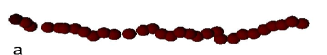
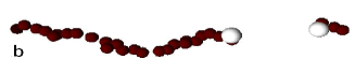
Figure 4: Snapshots of a chain with $30$ beads fixed at the left end while the right end is pulled by a constant force: (a) an equilibrated initial conformation, (b) a broken chain with the beads at the scission site shown in white.

We start the simulation with each bead separated by a distance equal to the equilibrium separation of the effective bond potential $U(y_{n})$ (eq. (102)); we then let the chain equilibrate with its environment using a Langevin thermostat. The number of integration steps for equilibration of a chain with $10$ atoms in $1$-D is $20000$ and the number of equilibrating integration steps is increased linearly as the chain length is increased. Because of the presence of the external pulling force, the stretched chain attains equilibrium only locally and not globally, i.e., it never turns into a coil. This justifies the linear increase in the number of equilibration steps with increase in chain length as opposed to “quadratic” as in the Rouse model. Once equilibration is achieved, time is set to zero and one measures the elapsed time (in MD time units) before any of the bond lengths extends beyond the distance separating the metastable minimum from the maximum, i.e., until one of the beads crosses the barrier (see Fig. 4). We repeat the above procedure for a large number of events ($5\times 10^{4}\div 2\times 10^{7}$) so as to sample the stochastic nature of rupture and calculate properties like the mean rate of rupture, the distribution of breaking bonds regarding their position in the chain, the (First Passage Time) FPT distribution, etc., for chains of different length in both $3d$ and $1d$. As one of our principle objectives, we also investigate the issue of chain recombination (self-healing) which is frequently observed after a scission event occurs. We demonstrate that the mere barrier crossing is not a reliable criterion for chain breakage since the majority of broken bonds are observed to recombine. Therefore we develop an unambiguous criterion for true rupture as illustrated in a later subsection.

IV.1 Chain Scission - Simulation Results

We compare here the simulation results with our theoretical prediction for the rupture probability of the $n$-th bond in a chain with $N$ bonds. The probability for bond scission (or, exit probability, in the more general context of Section II), is given by eq. (99).

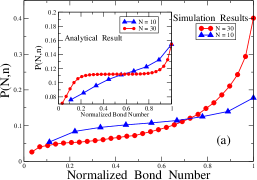
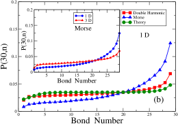
Figure 5: Normalized rupture probability vs consecutive bond number for chains with length $N$, subject to tensile force $f=0.25$, and friction $\gamma=0.25$: (a) $1D$ results for $E_{b}/k_{B}T=5$ and $N=10,\;30$. The consecutive number of the bonds is normalized as $n/N$ for convenience. Insert shows the theoretical prediction. (b) Theoretical prediction for $N=30$ along with simulation results for the Morse potential and the Double Harmonic potential. Inset shows the same for a chain with Morse interactions in both 1D and 3D.

In Fig. 5 the normalized rupture probability for chains (with $N=10$ and $N=30$) is shown with respect to the consecutive number of the individual bonds. The theoretical prediction, which follows from the numerical solution of eqs. (213), (214) and (215), is given in the inset. Both the theory- and MD-results indicate that the pulled end of the chain and the bonds in its vicinity break more frequently due to more freedom than those around the fixed end. Generally, the probability of rupture decreases steadily from the pulled end to the fixed end. For the longer chain, the end effects are not felt by the middle part of the chain and the probability of rupture $P(N,n)$ is nearly uniform forming a plateau-like region all over the length of the chain except at the ends. This feature is more pronounced in the theoretical rather than in the MD results. Such a comparison between the theory and MD-simulation findings has not been done before and could be viewed as a test for the merits and shortcomings of Kramers approach. Moreover, we believe that this reflects the incorporation of the collective unstable mode given in Sec. III.4.

One may assume that the detected discrepancy between theory and MD-simulation can be ascribed to the use of harmonic approximation around the metastable minimum and unstable maximum of the effective bond potential. To show this, we replaced the effective potential by a Double Harmonic potential - a parabola, and an inverted parabola, which approximates the effective potential in shape. The comparison of the three results - theoretical prediction, simulation with Morse potential, and simulation with the Double Harmonic potential is shown in Fig. 5b. Evidently, the rupture probability distribution for the Double Harmonic potential exposes also a plateau-like region and matches the theoretical prediction quite closely. So we infer that the absence of the plateau in case of the Morse potential can be ascribed to its anharmonicity. In the inset of Fig. 5b, we show the simulation results with the Morse potential for a $30$-atom chain in $1D$ and $3D$. Interestingly, one may see that the MD-results in $3D$ indicate a flatter distribution $P(N,n))$ than in $1D$, coming thus closer to theoretical predictions. As far as in $3D$ there exist much more configurations with endangered bonds due to transversal displacements of the beads, bond length fluctuations are suppressed as compared to $2D$ and the bond anharmonicity is less pronounced.

Theory predicts that the first passage time distribution goes asymptotically as $W\sim\exp(-t/\tau)$ ( see eq.(82)). In Fig. 6, we plot the FPT distribution for a chain with $30$ beads. One should note here the considerable difference of $W(\tau)$ between $1D$ and $3D$. The long time tail of the distribution is indeed seen to decay exponentially. We estimate the mean FPT (for the whole chain and not of an individual bond) as $\tau_{1D}=83.2$ and $\tau_{3D}=36.0$. The theoretical estimate for a $30$-bead chain in $1D$ is $\tau_{1D}\simeq 866.5$ which is an order-of-magnitude larger than that estimated from the simulations. This finding is in agreement with the results of Sain et al. - cf. Table I in Sain .

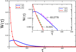
Figure 6: First passage time distributions $W(\tau)$ against elapsed time $\tau$ in $1D$ and $3D$ for a chain with $N=30$, $f=0.25$ and $\gamma=0.25$. The inset shows the same in semilog coordinates.

While assessing these results one should bear in mind that, as mentioned above, an event of bond scission can be defined as ”barrier crossing” whereby an endangered bond stretches beyond the position of the maximum of our potential $U(y)$. As has been discussed in the previous section, this position of the barrier depends on the externally applied force once the parameters of the Morse potential are fixed. For an applied force of magnitude $0.25$, the barrier position corresponds to a critical bead-bead separation (bond length) of $2.92$. Since frequently such scission event is immediately followed by recombination (that is, by self-healing of the bond), in what follows we have also considered a more stringent criterion for irreversible rupture. As a possible choice for the critical bead-bead separation one may take the larger value of $5$ which renders self-healing events virtually improbable (see below).

It is of interest to examine the dependence of mean FPT $\langle\tau\rangle$ on temperature $T$ for a given applied force $f$. In Fig.7 we show the change in FPT for irreversible rupture (and not barrier crossing) on inverse temperature for $f=0.25$ and $\gamma=0.25$. As expected from eq.(217), the Arrhenian nature of this relationship is clearly manifested in a semilog plot. From the exponentially fitted values, the effective barrier height is estimated to be $0.176$ in $1$D and $0.205$ in $3$D. The theoretical estimate of the barrier for a force of magnitude $0.25$ is $\Delta E_{b}\sim 0.27$. The somewhat lower value of the effective barrier has also been observed earlier in simulations with the Lennard-Jones potential for the fixed strain ensemble Oliveira_1 .

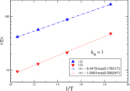
Figure 7: Mean first passage time $\langle\tau\rangle$ vs inverse temperature for a chain with $N=30$, $f=0.25$ and $\gamma=0.25$.

Eventually, in Fig. 8 we show the $N$-dependence of the mean FPT $\langle\tau\rangle$ and the average scission rate for both the Morse chain and the double-harmonic chain. We recall that we considered the unstable collective mode in Section IIID as the one responsible for the rupture event. Therefore, one might expect that the $N$-dependence of the scission rate would clearly reveal the degree of collectivity in bond breaking. Indeed, a linear increase in the scission rate with growing chain length would indicate the independent character of scission events, that is, the breakage of a single bond occurs irrespective of the neighboring bonds. In contrast, if the nature of bond scission is a strongly collective process, this $N$-dependence should be negligible. Evidently, Fig. 8 is a clear manifestation of the latter, contrary to an earlier assumption Oliveira_4 ; Sain ; Sokolov_1 ; Sokolov_2 that the total probability for scission of polymer with $N$ bonds is $N$ times that of a single bond. One sees a negligible decline in the mean FPT in Fig. 8a which appears as a very weak rise in the total rate in Fig. 8b, much weaker (with slope $\approx 0.1$) than the presumed linear growth with $N$.

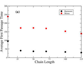
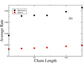
Figure 8: Mean first passage time $\langle\tau\rangle$ (a) and average scission rate (b) vs chain length $N$ for Morse and double-harmonic chains with $f=0.25$ and $\gamma=0.25$.

A visible finite size effect is detected only for $N=10$, indicating a strong influence of the boundaries (i.e., of the chain ends). This effect is easily understood from the inset to Fig. 5a where the absence of a plateau suggests that the bonds in the short chain are not equivalent. One can also verify from Fig. 8 that the double-harmonic chain breaks faster than the Morse one,

IV.2 The breaking of a bond

We now examine the expansion rate of the breaking bond. Theory predicts that the length of the endangered bond extends with time as $\exp(-\kappa t)$ (see eq. (16)), where $\kappa$, the transmission factor given by eq. (215), is negative.

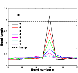
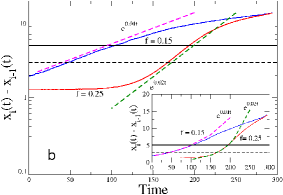
Figure 9: Stretching of a breaking ($15$-th) bond with time in a chain with $30$-beads for $f=0.15$ and $f=0.25$: (a) Evolution of the lengths of a breaking bond and of its neighbors. The dashed line denotes an extension equal to the barrier position. (b) Variation of the length of a breaking bond with time in semi-logarithmic coordinates. Dashed lines indicate exponential increase in agreement with theoretical predictions. The inset shows the expansion in normal coordinates for visual aid. The length growth has been monitored up to an expansion of $15$, well beyond the location of the barrier. Data has been averaged over many events. The dashed black line shows the position of the barrier while the solid line marks an expansion of 5.0, later set as the criterion for irreversible rupture for an applied force $f=0.25$.

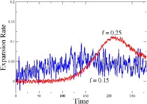
Figure 10: Mean expansion rate of the breaking $15$-th bond.

Exponential fits of the growth curves around the position of the barriers ($\sim 2.92$ for $f=0.25$ and $\sim 3.05$ for $f=0.15$) give $|\kappa|\sim 0.01$ for $f=0.15$ and $|\kappa|\sim 0.02$ for $f=0.25$ is given in Fig.9. Analytical calculations yield $0.11$ and $0.22$ - Fig. 9 - respectively, an order of magnitude higher than that estimated from the simulations and consistent with the result obtained earlier from the lifetime distribution.

Eventually, we show the rate of expansion of the monitored bond for two different forces, note that the exponential character of the curves is best pronounced when the growing bond length is in the vicinity of the barrier (hump) position which is indicated in Fig. 9 by horizontal lines, in agreement with the theoretical predictions, eq.(16). The speed of expansion itself is displayed in Fig. 10 (statistic fluctuations are strongly pronounced for the weaker tension $f=0.15$) which demonstrates that also the speed of bond extension attains a maximum at the moment it goes over the barrier position.

V Self-Healing (Recombination) of Broken Bonds

The process of bond breakage is not fully described by the escape from the metastable well and the barrier crossing. Once the barrier has been surmounted, the ”endangered bond” could further increase its length up to a critical value which still leaves the possibility for eventual return and healing of the chain. In contrast, beyond this critical value the healing probability gets negligibly small and the chain breaks irreversibly. This healing process has been pointed out earlier Sebastian and observed in a MD-simulation Bolton . Below we suggest a theoretical description of the process of recombination and derive analytical expressions for the healing time and distance distribution function. One should bear in mind that it is the thermal fluctuations that initiate recombination events while the downhill ramp potential of the applied tensile force always acts in the opposite ”destructive” direction. This potential may still be approximated by an inverted parabola before the ”endangered bond” length approaches a critical size whereby the two pieces of the chain would move apart irreversibly.

V.1 Theory

As far as the healing process is largely localized on the ”endangered bond”, it may be treated as an effectively one-dimensional problem. The corresponding Fokker-Planck equation for the probability distribution function of positions (in our case - “endangered” bond lengths) and velocities (bond length velocities) is known as Kramers equationKramers and has been used to describe reaction kinetics. The complete solution of the Kramers equation for the harmonic as well as inverted harmonic (or inverted parabolic) potential was Fig. 8 given by Risken Risken .

Consider the Kramers equation for the inverted harmonic potential $U(x)=-\Omega_{2}^{2}x^{2}/2$, assumed to represent the top of the barrier. The coordinate-velocity transition probability $P(x,v,t|x^{\prime},v^{\prime},0)$ is governed by the following equation (see Sec. 10 in Risken ):

$$\dfrac{\partial}{\partial t}\>P=-\dfrac{\partial}{\partial x}[vP]+\dfrac{\partial}{\partial v}\>[(U^{\prime}(x)+\gamma v)P]+\gamma\>v_{\rm th}^{2}\>\dfrac{\partial^{2}}{\partial v^{2}}\>P$$ (218)

where the thermal velocity $v_{\rm th}=\sqrt{T/m}$ and the initial conditions are fixed as $P(x,v,t=0|x^{\prime},v^{\prime},0)=\delta(x-x^{\prime})\>\delta(v-v^{\prime})$. The general solution of eq. (218) is given by Risken and is relegated to Appendix C.

V.1.1 Healing time distribution function

One may treat the healing time distribution function by noting that the process starts at the top of the inverted harmonic potential $U(x)=-\Omega_{2}^{2}\>x^{2}/2$, where $x^{\prime}=0$ and $v^{\prime}=|\kappa|$ . The coordinate of the turning point (healing distance) is counted with respect to $x=0$ whereas the velocity at that point might be arbitrary within the interval $-\infty\leq v\leq 0$ (i.e., the return velocity is pointing to the left). Thus, the healing time PDF can be obtained from the transition probability eq. (263) as

$$P_{\rm heal}(t)=\int\limits_{-\infty}^{0}\>dv\>P(0,v,t|0,|\kappa|,0)$$ (219)

After explicit integration in eq. (219) and taking into account eq. (270), one obtains

$$P_{\rm heal}(t)=\dfrac{1}{2}\sqrt{\dfrac{1}{2\pi\sigma_{xx}(t)}}\>\exp\left\{-\dfrac{x^{2}(t)}{2\sigma_{xx}(t)}\right\}\left\{1-{\rm erf}\left[\dfrac{\sigma_{xx}(t)\>v(t)-\sigma_{xv}(t)\>x(t)}{\sqrt{2\sigma_{xx}(t)\det{\bm{\sigma}}}}\right]\right\}$$ (220)

where the error function ${\rm erf}(z)=(2/\sqrt{\pi})\int_{0}^{z}\>{\rm e}^{-x^{2}}dx$, and $x(t)$, $v(t)$ are given by eq. (271) (with $x^{\prime}=0$ and $v^{\prime}=|\kappa|$).

V.1.2 Healing distance distribution function

In order to determine the distribution of distances $h$ from the hump at $x=0$ where the extending bond may still turn back to shrinking, one may consider the PDF for the maximal divergence distance $Q(h)$ before the bond returns and heals. In this case a critical value $h_{c}$ can be defined as a point where $Q(h)$ gets very small.

One may express $Q(h)$ in terms of the transition probability $P(x,v,t|x^{\prime},v^{\prime},t^{\prime})$ by taking into consideration the following arguments. The overall return process can be seen as the composition (recall that the process is Markovian) of two processes. The first one starts from the top of the inverted harmonic potential with the initial $x^{\prime}=0$ and $v^{\prime}=|\kappa|$ and continues down the ramp until a turning point $x=h$ where the velocity becomes zero, i.e., $v=0$, at an intermediate time moment $t^{\prime}$. The probability of this process is given by $P(h,0,t^{\prime}|0,|\kappa|,0)$. The reverse process starts from the turning point (i.e., $x^{\prime}=h,v^{\prime}=0$) at time moment $t^{\prime}$, and continues back to the top of the potential where $x=0$ and the velocity can be any in the interval $-\infty\leq v\leq 0$. The latter means that the corresponding transition probability should be integrated over velocity, i.e., $\int_{-\infty}^{0}dvP(0,v,t|h,0,t^{\prime})$. Finally, since the total time interval may also be arbitrary, one should integrate over times. Thus, one obtains

$$Q(h) = \int\limits_{0}^{\infty}dt\int\limits_{0}^{t}dt^{\prime}\int\limits_{-\infty}^{0}dv\>P(0,v,t|h,0,t^{\prime})\>P(h,0,t^{\prime}|0,|\kappa|,0)$$

$$= \underbrace{\int\limits_{0}^{\infty}d\tau\int\limits_{-\infty}^{0}dv\>P(0,v,\tau|h,0,0)}_{I(h)}\>\underbrace{\int\limits_{0}^{\infty}dt^{\prime}P(h,0,t^{\prime}|0,|\kappa|,0)}_{J(h)}=I(h)\>J(h)$$

where we have changed the order of time integration. Taking into account the form of the transition probability, eq. (263), and after integrating over the velocity, the expression for $I(h)$ reads

$$I(h)=\dfrac{1}{2}\>\int\limits_{0}^{\infty}dt\sqrt{\dfrac{1}{2\pi\sigma_{xx}(t)}}\>\exp\left\{-\dfrac{x^{2}(t)}{2\sigma_{xx}(t)}\right\}\left\{1-{\rm erf}\left[\dfrac{\sigma_{xx}(t)v(t)-\sigma_{xv}(t)x(t)}{\sqrt{2\sigma_{xx}(t)\det{\bm{\sigma}}}}\right]\right\}$$ (221)

where $x(t)$ and $v(t)$ are given by

$$x(t) = G_{xx}(t)\>h$$

$$v(t) = G_{vx}(t)\>h$$ (222)

By making use of the expressions for the inverse $\sigma$-matrix, eq. (270), the expression for $J(h)$ takes on the form

$$J(h)=\dfrac{1}{2\pi}\>\int\limits_{0}^{\infty}dt\dfrac{1}{\sqrt{\det{\bm{\sigma}}}}\>\exp\left\{-\dfrac{\sigma_{vv}(t)[h-x(t)]^{2}+2\sigma_{xv}(t)[h-x(t)]v(t)+\sigma_{xx}(t)v^{2}(t)}{2\det{\bm{\sigma}}}\right\}$$ (223)

with

$$x(t) = G_{xv}(t)\>|\kappa|$$

$$v(t) = G_{vv}(t)\>|\kappa|\;.$$ (224)

V.2 MD-simulation of Self-Healing

The simulation scheme for sampling the self-healing distributions is as follows - once the largest bond in the chain crosses the barrier position, one monitors its expansion for $1000$ integration steps and records the maximum expansion and the time spent before it crosses back the barrier. Frequently such a pseudo-broken bond heals again so that from the above record, one may recover the distribution of the maximum expansion beyond the barrier, and the time spent in a pseudo-broken state before the healing occurs.

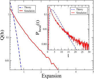
Figure 11: Probability distribution of healing bond lengths and healing times (inset) for a $30$-bead chain in $1$D and $f=0.25$. Both plots are shown in semilog coordinates. Dashed lines denote theoretical predictions.

In Fig. 11 we show the distribution of the healing lengths and healing times (inset) obtained from simulations and from theory. Evidently, the healing time distribution $P_{\rm heal}(t)$ looks qualitatively identical for both the theoretical treatment (which is based on eq. (220))and the simulations: there is a maximum just beyond the barrier crossing event for $t\neq 0$ and a fast (exponential) decay thereafter. The existence of the maximum can be attributed to the thermostat - just after crossing the barrier one has to wait for a while a thermal kick turns the trajectory into reverse direction. On the other hand, for longer time intervals the downhill motion wins (i.e., the healing becomes progressively improbable) and $P_{\rm heal}(t)$ decreases rapidly with time.

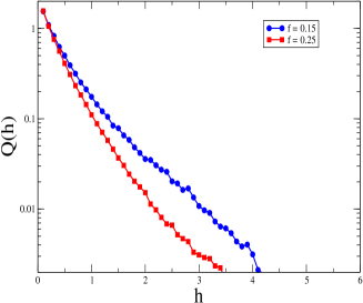
Figure 12: The healing expansion distribution $Q(h)$ for $f=0.15$ and $f=0.25$ plotted in semi-logarithmic coordinates. The zero of the x-axis corresponds to the barrier positions, which are different for the two different values of the force.

The distribution of the healable expansions beyond the barrier is of greater importance because it sets a more stringent criterion of true (irreversible) rupture. We see that for $f=0.25$, the probability of healing is negligible for an expansion of $\sim 2.0$ beyond the barrier, i.e., a bond expansion of $2.92+2.0\approx 5.0$. Once the expansion of the bond reaches $h_{c}\approx 5.0$ for $f=0.25$, it is highly unlikely for the bond to heal. One should note that the process is stochastic in nature so that a bond that has expanded even beyond $h_{c}$ may still manage to heal. Such an event, however, is highly unlikely and the criterion defined in the above manner serves to be a good one for all practical purposes. The theoretical distribution (calculated according to eqs. (V.1.2), (221) and (223)), decays much faster than that obtained from simulations; this is because of the faster descent of the quadratic potential (considered in theory within the linearized approximation) as compared to the roughly linearly decaying effective potential beyond the barrier.

How does the above picture change when the conditions of the simulation are varied? To answer this question, we have performed simulations and we find that the above distribution does not vary much with friction, chain length or whether the simulation is performed in $1$D or $3$D. The distribution however depends on the applied tensile force as shown in Fig. 12 for two different forces.

As expected intuitively, the distribution decays faster for a larger force because healing is more unlikely in case of a steeper unstable potential beyond the barrier. From a practical point of view, such a distribution for several different forces can be very helpful in determining a criterion for irreversible rupture.

We next turn to the question of the dependence of the healing on temperature.

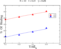
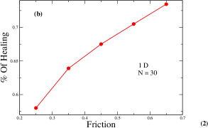
Figure 13: (a) The healing fraction for $f=0.25$ and $\gamma=0.25$ at different values of the temperature. A power-law regression gives an exponent of $\sim 0.2$ in $1$D and $\sim 0.3$ in $3$D. (b) Increase of the fraction of self-healing bonds with friction $\gamma$.

Figure 13 shows the fraction of self-healing events on the temperature for $f=0.25$ and $\gamma=0.25$. As expected, healing becomes more frequent as the temperature is increased because the bead that has crossed the barrier now receives stronger thermal kicks capable of sending it back over the barrier. One can also see that for the same temperature, healing is (understandably) more frequent in $1D$ than in $3D$. The effect of growing friction $\gamma$ is similar, on the one hand it strengthens kicks by the thermostat on the beads at the verge of breaking, and on the other hand it delays such beads in “rolling down” the downhill ramp potential, providing more time to receive a thermal kick which could turn them back.

VI Conclusion

In the present work we have studied the process of polymer chain breakage for linear chains subjected to constant tensile force by multidimensional Kramers-Langer approach and compared theoretical predictions to results of extensive MD simulations in one- and three dimensions. The adopted theoretical treatment makes it possible to consider collective unstable modes as being mainly responsible for chain scission. Comparison with simulation data as, for example, the distribution of the probability for scission over bond index, the scission time distribution, variation of MFPT with temperature and chain length as well as the bond breaking dynamics indicates that the Kramers-Langer approach agrees qualitatively with observations.

We demonstrate that the recombination (self-healing) dynamics of the breaking bonds can be qualitatively reproduced by the Kramers equation. We derive analytic expressions for the healing time and expansion distributions in reasonable agreement with the MD data and reveal the variation of the fraction of healing bonds with temperature and friction. In fact, we demonstrate that more that $50\%$ of the crossings of the activation barrier end up as healed bonds again (this fraction changes with temperature) especially in the $3D$ simulations. This finding should be kept in mind in the assessment of earlier research work where only $1D$ simulations of breaking chains have been performed and bond-healing was not allowed for.

One should emphasize, however, that we still find a discrepancy of nearly an order of magnitude between theory and computer experiment regarding the mean rate of scission, that is, the rate of bond breaking is significantly underestimated by theory (cf. also Sain ). We believe that the origin of this discrepancy is related to the existence of non-linear localized excitations (breathers) in the anharmonic lattice which remain out of the scope of this investigation. Recent studies Peyrard indicate the breathers play very important role regarding energy transfer in discrete non-linear chains which serve a generic model for biopolymers. Clearly, furter research in this direction is needed before a good understanding of the whole problem is reached.

VII Acknowledgments

We are indebted to B. Dünweg and L. Manevitch for helpful discussions in the course of this study. This work has been supported by the Deutsche Forschungsgemeinschaft (DFG), Grant No. SFB 625/B4.

Appendix A Calculation of $\sum_{i,j}\nu_{i}\Gamma_{ij}\nu_{j}$

Let us calculate $\sigma\equiv\sum_{i,j}\nu_{i}\Gamma_{ij}\nu_{j}$ which occurs in eq. (93). Because $\sum_{i=1}^{2N}\nu_{i}^{2}=1$ this can be seen as a eigenvalue problem, i.e.

$$\sum_{i=1}^{2N}\>\nu_{i}\>\Gamma_{ij}=\sigma\nu_{j}$$ (225)

The corresponding characteristic equation reads

$$\det[\Gamma_{ij}-\delta_{ij}\sigma]=0$$ (226)

The matrix $\Gamma_{ij}$ has a block structure (see eq. (53)) so that eq. (226) takes the form

$$\det\left(\begin{array}[]{ccc}\begin{array}[]{ccc}-\sigma&\cdots&0\\ \vdots&&\vdots\\ 0&\cdots&-\sigma\end{array}&&\begin{array}[]{ccc}0&\cdots&0\\ \vdots&\ddots&\vdots\\ 0&\cdots&0\end{array}\\ \begin{array}[]{ccc}0&\cdots&0\\ \vdots&\ddots&\vdots\\ 0&\cdots&0\end{array}&&\begin{array}[]{ccc}m\gamma-\sigma&\cdots&0\\ \vdots&\ddots&\vdots\\ 0&\cdots&m\gamma-\sigma\end{array}\end{array}\right)=0$$ (241)

On the other hand the determinant of he block-diagonal matrix $\det\left(\begin{smallmatrix}{\bf A}&{\bf 0}\\ {\bf 0}&{\bf D}\end{smallmatrix}\right)=\det{\bf A}\det{\bf D}=(-\sigma)^{N}(m\gamma-\sigma)^{N}=0$. As a result

$$\sigma=m\gamma$$ (242)

Appendix B How to calculate the determinant of a symmetrical tridiagonal matrix

The typical tridiagonal $N\times N$-matrix which is common in the context of one-dimensional string of beads model has the following form

$${\cal T}(N)=\left(\begin{array}[]{rrrrrr}2&-1&&&&{\bf 0}\\ -1&2&-1&&&\\ 0&-1&2&-1&&\\ &\ddots&\ddots&\ddots&\ddots\\ &&\ 0&-1&2&-1\\ {\bf 0}&&&&-1&1-\beta\end{array}\right)$$ (249)

where $\beta$ is an arbitrary rational number. To calculate the determinant we use the Laplace’s formula Lancaster which holds that for an arbitrary matrix $A$ the determinant $\det(A)=\sum_{j=1}^{N}\>A_{ij}(-1)^{i+j}M_{ij}$ where $M_{ij}$ is the minor (i.e. the determinant of the matrix that results from A by removing the i-th row and the j-th column). By making use this formula for the matrix in eq.(249) with respect to the first row and expanding similarly again, one finds the recurrence relation

$$\det[{\cal T}(N)]=2\det[{\cal T}(N-1)]-\det[{\cal T}(N-2)]$$ (250)

This reccurence relation to be solved needs two initial conditions

$$\det[{\cal T}(1)]=1-\beta\qquad\det[{\cal T}(2)]=\det\left(\begin{array}[]{rr}2&-1\\ -1&{1-\beta}\end{array}\right)=1-2\beta$$ (253)

Thus

$$\begin{array}[]{lllllll}&\det[{\cal T}(3)]&=&2(1-2\beta)&-&{1+\beta}&=1-3\beta\\ \\ &\det[{\cal T}(4)]&=&2(1-3\beta)&-&{1+2\beta}&=1-4\beta\\ \\ \lx@intercol\dotfill\hfil\lx@intercol\\ \\ &\det[{\cal T}(N)]&=&{1-\beta N}&&&\end{array}$$ (261)

As a result we can finally write down

$$\det[{\cal T}(N)]=(1-\beta N)$$ (262)

Appendix C Solution of one-dimensional Kramers equation

The general solution of eq. (218) reads Risken

$$P(x,v,t|x^{\prime},v^{\prime},0) = \dfrac{1}{2\pi(\det{\bm{\sigma}})^{1/2}}\>\exp\Bigl{\{}-\dfrac{1}{2}[{\bm{\sigma}}^{-1}(t)]_{xx}\>[x-x(t)]^{2}-[{\bm{\sigma}}^{-1}(t)]_{xv}\>[x-x(t)]\>[v-v(t)]$$ (263)

$$- \dfrac{1}{2}[{\bm{\sigma}}^{-1}(t)]_{vv}\>[v-v(t)]^{2}\Bigr{\}}$$

where the $2\times 2$ $\sigma$-matrix

$$\sigma_{ij}(t)=\left(\begin{array}[]{cc}\sigma_{xx}(t)&\sigma_{xv}(t)\\ \sigma_{xv}(t)&\sigma_{vv}(t)\end{array}\right)$$ (266)

has the following elements has the following elements

$$\sigma_{xx}(t) = \dfrac{\gamma v_{\rm th}^{2}}{(\lambda_{1}-\lambda_{2})^{2}}\>\left[\dfrac{\lambda_{1}+\lambda_{2}}{\lambda_{1}\lambda_{2}}+4\dfrac{{\rm e}^{-(\lambda_{1}+\lambda_{2})t}-1}{\lambda_{1}+\lambda_{2}}-\dfrac{{\rm e}^{-2\lambda_{1}t}}{\lambda_{1}}-\dfrac{{\rm e}^{-2\lambda_{2}t}}{\lambda_{2}}\right]$$

$$\sigma_{xv}(t) = \dfrac{\gamma v_{\rm th}^{2}}{(\lambda_{1}-\lambda_{2})^{2}}\>\left[{\rm e}^{-\lambda_{1}t}-{\rm e}^{-\lambda_{2}t}\right]^{2}$$

$$\sigma_{vv}(t) = \dfrac{\gamma v_{\rm th}^{2}}{(\lambda_{1}-\lambda_{2})^{2}}\>\left\{\lambda_{1}+\lambda_{2}+\dfrac{4\lambda_{1}\lambda_{2}}{\lambda_{1}+\lambda_{2}}\>[{\rm e}^{-(\lambda_{1}+\lambda_{2}}-1]-\lambda_{1}\>{\rm e}^{-2\lambda_{1}t}-\lambda_{2}\>{\rm e}^{-2\lambda_{2}t}\right\}$$ (267)

and where the eigenvalues $\lambda_{1}$ and $\lambda_{2}$ are

$$\lambda_{1} = \dfrac{1}{2}(\gamma+\sqrt{\gamma^{2}+4\Omega_{2}^{2}})$$ (268)

$$\lambda_{2} = \dfrac{1}{2}(\gamma-\sqrt{\gamma^{2}+4\Omega_{2}^{2}})=\kappa<0$$ (269)

We underline that the negative eigenvalue $\lambda_{1}$ is nothing but the transmission factor $\kappa$ given by eq. (215) whereas the characteristic frequency $\Omega_{2}$ is given by eq. (105). The determinant and the inverse $\sigma$-matrix in eq. (263) are defined as as follows

$$\det{\bm{\sigma}} = \sigma_{xx}\sigma_{vv}-\sigma_{xv}^{2}$$

$$({\bm{\sigma}}^{-1})_{xx} = \dfrac{\sigma_{vv}}{\det{\bm{\sigma}}}$$

$$({\bm{\sigma}}^{-1})_{xv} = ({\bm{\sigma}}^{-1})_{vx}=-\dfrac{\sigma_{xv}}{\det{\bm{\sigma}}}$$

$$({\bm{\sigma}}^{-1})_{vv} = \dfrac{\sigma_{xx}}{\det{\bm{\sigma}}}$$ (270)

The mean values $x(t)$ and $v(t)$ in eq. (263) are given by

$$x(t) = G_{xx}(t)\>x^{\prime}+G_{xv}(t)\>v^{\prime}$$

$$v(t) = G_{vx}(t)\>x^{\prime}+G_{vv}(t)\>v^{\prime}$$ (271)

where the Green function matrix elements read

$$G_{xx}(t) = \dfrac{\lambda_{1}{\rm e}^{-\lambda_{2}t}-\lambda_{2}{\rm e}^{-\lambda_{1}t}}{\lambda_{1}-\lambda_{2}}$$

$$G_{xv}(t) = \dfrac{{\rm e}^{-\lambda_{2}t}-{\rm e}^{-\lambda_{1}t}}{\lambda_{1}-\lambda_{2}}$$

$$G_{vx}(t) = \lambda_{1}\lambda_{2}\>\dfrac{{\rm e}^{-\lambda_{1}t}-{\rm e}^{-\lambda_{2}t}}{\lambda_{1}-\lambda_{2}}$$

$$G_{vv}(t) = \dfrac{\lambda_{1}{\rm e}^{-\lambda_{1}t}-\lambda_{2}{\rm e}^{-\lambda_{2}t}}{\lambda_{1}-\lambda_{2}}$$ (272)

References

• (1) H. -H. Kausch, Polymer Fracture, Springer-Verlag, New York, 1987.
• (2) B. Crist, Ann. Rev. Mater. Sci. 25, 295 (1995).
• (3) L. Garnier, B. Gauthier-Manuel, E.W. van der Vegte, J. Snijders, G. Hadziioannou, J. Chem. Phys. 113, 2497 (2000).
• (4) M.Grandbois, M. Beyer, M. Rief, H. Clausen-Schaumann, H. E. Gaub, Science 283, 1728 (1999).
• (5) A. M. Saitta, M. L. Klein, J. Phys. Chem. A 105, 6495 (2001).
• (6) A. M. Maroja, F. A. Oliveira, M. Ciesla, L. Longa, Phys. Rev. E 63, 061801 (2001).
• (7) U. F. Rohrig, I. Frank, J. Chem. Phys. 115, 8670 (2001).
• (8) D. Gersappe, M. O. Robins, Europhys. Lett. 48, 150 (1999).
• (9) A. E. Filipov, J. Klafter, M. Urbakh, Phys. Rev. Lett. 92, 135503 (2004).
• (10) D. Aktah, I. Frank, J. Amer. Chem. Soc. 124, 3402 (2002).
• (11) M. K. Beyer, H.Clausen-Schaumann, Chem. Rev. 105, 2921 (2005).
• (12) S. A. Harris, Contemp. Phys. 45, 11 (2004).
• (13) Y. V. Perverzev, O. V. Prezhdo, Phys. Rev. E 73, 050902 (2006).
• (14) F. Bueche, J. Appl. Phys. 29, 1231 (1958).
• (15) S. N. Zhurkov, V.E. Korsukov, J. Polym. Sci. (Pol. Phys. Ed.) 12, 385 (1974).
• (16) T.P. Doerr, P.L. Taylor, J. Chem. Phys. 101, 1017 (1994)
• (17) C. F. Lee, Phys. Rev. E 80, 031134 (2009)
• (18) J. N. Stember, G. S. Ezra, Chem. Phys. 337, 11 (2007).
• (19) K. Bolton, S. Nordholm, H.W. Schranz, J. Phys. Chem. 99, 2477 (1995).
• (20) R. Puthur, K.L. Sebastian, Phys. Rev. B 66, 024304 (2002)..
• (21) F. A. Oliveira, P.L. Taylor, J. Chem. Phys. 101, 10118 (1994).
• (22) F. A. Oliveira, Phys. Rev. B 52, 1009 (1995).
• (23) F. A. Oliveira, J. A. Gonzalez, Phys. Rev. B 54, 3954 (1996).
• (24) F. A. Oliveira, Phys. Rev. B 57, 10578 (1998).
• (25) H.A. Kramers, Physica (Utrecht) 7, 284 (1940).
• (26) A. Sain, C.L. Dias, M. Grant, Phys. Rev. E 74, 046111 (2006).
• (27) J. S. Langer, Ann. Phys. (N.Y.) 54, 258 (1969).
• (28) P. Hänngi, P. Talkner, M. Borkovec, Rev. Mod. Phys. 62, 251 (1990).
• (29) B.J. Matkowsky, Z. Schuss, SIAM J. App. Math. 33, 365 (1977).
• (30) C. W. Gardiner, Handbook of Stochasic Methods, Springer-verlag, Berlin, 2004.
• (31) H. Risken, The Fokker-Planck Equation, Springer-Verlag, Berlin, 1989.
• (32) H. Goldstein, Classical Mechanics, Addison-Wesly, Reading, Harvard University, Cambridge, 1980.
• (33) P. Lancaster, M. Tismenetsky, The Theory of Matrices, Academic Press, N.Y. , 1985.
• (34) H. A. Weidenmüller, Z. Jing-Shang, J. Stat. Phys. 34, 191 (1984).
• (35) P. Talkner, Z. Phys. B 68, 201 (1987).
• (36) S.N. Elaydi, An Introduction to Difference Equations, Springer-Verlag, N.Y., 1999.
• (37) S. Fugmann, I.M. Sokolov, Phys. Rev. E 79, 021803 (2009).
• (38) S. Fugmann, I.M. Sokolov, Europhys. Lett. 86, 28001 (2009).
• (39) M. Peyrard and Y. Sire, in Energy Localisation and Transfer, Ed. T. Dauxois, World Scientific, London, 2004, p. 325.