Collinear antiferromagnetic state in a two-dimensional Hubbard model at half filling

Abstract

In a half-filled Hubbard model on a square lattice, the next-nearest-neighbor hopping causes spin frustration, and the collinear antiferromagnetic (CAF) state appears as the ground state with suitable parameters. We find that there is a metal-insulator transition in the CAF state at a critical on-site repulsion. When the repulsion is small, the CAF state is metallic, and a van Hove singularity can be close to the Fermi surface, resulting in either a kink or a discontinuity in the magnetic moment. When the on-site repulsion is large, the CAF state is a Mott insulator. A first-order transition from the CAF phase to the antiferromagnetic phase and a second-order phase transition from the CAF phase to the paramagnetic phase are obtained in the phase diagram at zero temperature.

I introduction

In a hall-filled Hubbard model Hubbard63 with only nearest-neighbor (NN) hopping, the spin exchange between NN electrons is antiferromagnetic, leading to the antiferromagnetic insulating ground state, the Néel state, on a square lattice. When the next-nearest-neighbor (NNN) hopping is present, there is also antiferromagnetic spin exchange between NNN electrons, which is destructive to the antiferromagnetic order. This spin frustration leads to a transition from the Néel state to a paramagnetic state at a critical on-site repulsion Lin87 ; Kondo95 ; Hofstetter98 . A metallic antiferromagnetic phase exists in a narrow region near this transition Duffy97 ; Yang99 ; Chitra99 . Another possible ground state found in numerical studies Imada01 ; Tocchio08 ; Tremblay08 due to spin frustration is the collinear antiferromagnetic (CAF) state in which the spin configuration is antiferromagnetic along one axis and ferromagnetic along the other axis. The transition from the Néel state to the CAF state in a Heisenberg model on a square lattice with both NN spin exchange $J>0$ and NNN spin exchange $J^{\prime}>0$ was proposed at $J^{\prime}=J/2$ Chandra90 , and the exact phase diagram of this model is still under investigation. In the $2d$-Hubbard model, properties of the CAF state are largely unknown.

In this work, we study properties of the CAF state in a half-filled Hubbard model on a square lattice at zero temperature. We find that there is a metal-insulator transition in the CAF state. The magnetic moment displays a kink at this transition point. When $U$ is small, the CAF state is metallic, and a van Hove singularity may be close to the Fermi energy. When $U$ is large, the CAF state is an insulator. The paramagnetic, antiferromagnetic, and CAF states are ground states in different regions of the phase space. There is a second-order transition between CAF and paramagnetic phases, and a first-order transition between CAF and antiferromagnetic phases. Based on these results, a zero-temperature phase diagram is obtained, in comparison with previous studies Lin87 ; Kondo95 ; Hofstetter98 ; Duffy97 ; Yang99 ; Chitra99 ; Li94 ; Valenzuela00 ; Imada01 ; Avella01 ; Taniguchi05 ; Yokoyama06 ; Japaridze07 ; Tocchio08 ; Tremblay08 ; Peters09 .

II Mean-field theory of the CAF state

The Hamiltonian of the Hubbard model with both NN and NNN hoppings is given by

$$\mathcal{H}=-t\sum_{\langle ij\rangle,\sigma}c_{i\sigma}^{\dagger}c_{j\sigma}+t^{\prime}\sum_{\langle ij\rangle^{\prime},\sigma}c_{i\sigma}^{\dagger}c_{j\sigma}+U\sum_{i}n_{i\uparrow}n_{i\downarrow},$$ (1)

where $c_{i\sigma}$ and $c_{i\sigma}^{\dagger}$ are electron annihilation and creation operators at site $i$ with spin $\sigma$, and $n_{i\sigma}=c_{i\sigma}^{\dagger}c_{i\sigma}$ is the number operator. The first two terms on r.-h.-s. of Eq. (1) describe NN and NNN hoppings, and the last term describes the on-site repulsion. The square lattice has total $N$ sites and the lattice constant is given by $a$.

In the large $U$ limit, the NN hopping leads to antiferromagnetic spin exchange $J=4t^{2}/U$ between NNs, and similarly $J^{\prime}=4t^{\prime 2}/U$ between NNNs. The energy per site of the classical antiferromagnetic state is $-(J-J^{\prime})/2$, while it is $-J^{\prime}/2$ in the classical CAF state. Thus intuitively when $J^{\prime}>J/2$ or equivalently $t^{\prime}>t/\sqrt{2}$, the CAF state is preferred over the antiferromagnetic state. However, much is unknown when the repulsion $U$ is of the same order as $t$ or $t^{\prime}$, which will be investigated in this work.

In both antiferromagnetic and CAF states, the square lattice can be divided into two sublattices. The order parameter is the same on each sublattice, but opposite on different sublattices. It can be generally written as

$$\langle n_{i\uparrow}\rangle-\langle n_{i\downarrow}\rangle=m\cos({\bf Q}\cdot{\bf r}_{i}),$$ (2)

where ${\bf r}_{i}$ is the coordinate of site $i$ and $m>0$ is the magnetic moment. In the antiferromagnetic state, the wavevector ${\bf Q}$ is given by ${\bf Q}=(\pi/a,\pi/a)$; in the CAF state, ${\bf Q}=(0,\pi/a)$ or ${\bf Q}=(\pi/a,0)$. When $m=0$, the order parameter is zero, and the system is in a paramagnetic state.

In the mean-field approach, the on-site repulsion term in the Hamiltonian can be approximated by

$$Un_{i\uparrow}n_{i\downarrow}\approx U(n_{i\uparrow}\langle n_{i\downarrow}\rangle+n_{i\downarrow}\langle n_{i\uparrow}\rangle-\langle n_{i\uparrow}\rangle\langle n_{i\downarrow}\rangle),$$ (3)

and the mean-filed Hamiltonian of the antiferromagnetic or CAF states can be written as

$$\mathcal{H}_{\rm MF}= - {UN\over 4}(n^{2}-m^{2})+\sum_{{\bf k}}[\sum_{\sigma}(\epsilon_{\bf k}+{Un\over 2})c_{{\bf k}\sigma}^{\dagger}c_{{\bf k}\sigma}$$ (4)

$$- {Um\over 2}(c_{{\bf k}\uparrow}^{\dagger}c_{{\bf k}+{\bf Q}\uparrow}-c_{{\bf k}\downarrow}^{\dagger}c_{{\bf k}+{\bf Q}\downarrow})],$$

where $\epsilon_{\bf k}=-2t(\cos k_{x}a+\cos k_{y}a)+4t^{\prime}\cos k_{x}a\cos k_{y}a$, $n\equiv\langle n_{i\uparrow}\rangle+\langle n_{i\downarrow}\rangle=1$ at half filling.

The mean-field Hamiltonian can be diagonalized by a standard canonical transformation

$$\mathcal{H}_{\rm MF} =\sum_{{\bf k}\sigma}{\rm{}^{\prime}}\left[\varepsilon_{{\bf k}}^{-}\alpha_{{\bf k}\sigma}^{\dagger}\alpha_{{\bf k}\sigma}+\varepsilon_{{\bf k}}^{+}\beta_{{\bf k}\sigma}^{\dagger}\beta_{{\bf k}\sigma}\right]-{UN\over 4}\left(n^{2}-m^{2}\right),$$ (5)

where the ${\bf k}$-summation is over the first Brillouin zone of a sublattice, the quasi-particle operators are given by $\alpha_{{\bf k}\uparrow}=u_{\bf k}c_{{\bf k}\uparrow}+v_{\bf k}c_{{\bf k}+{\bf Q}\uparrow}$, $\alpha_{{\bf k}\downarrow}=u_{\bf k}c_{{\bf k}\downarrow}-v_{\bf k}c_{{\bf k}+{\bf Q}\downarrow}$, $\beta_{{\bf k}\uparrow}=-v_{\bf k}c_{{\bf k}\uparrow}+u_{\bf k}c_{{\bf k}+{\bf Q}\uparrow}$, $\beta_{{\bf k}\downarrow}=v_{\bf k}c_{{\bf k}\downarrow}+u_{\bf k}c_{{\bf k}+{\bf Q}\downarrow}$, and the coefficients are given by

$$u_{\bf k}^{2}=1-v_{\bf k}^{2}={1\over 2}\left[1-{\epsilon_{\bf k}-\epsilon_{{\bf k}+{\bf Q}}\over\sqrt{(\epsilon_{\bf k}-\epsilon_{{\bf k}+{\bf Q}})^{2}+4\Delta^{2}}}\right],$$

with $\Delta=mU/2$. The quasi-particles form two bands, with energies given by

$$\varepsilon^{\pm}_{{\bf k}}={1\over 2}(\epsilon_{\bf k}+\epsilon_{{\bf k}+{\bf Q}}+Un)\pm{1\over 2}\sqrt{(\epsilon_{\bf k}-\epsilon_{{\bf k}+{\bf Q}})^{2}+4\Delta^{2}}.$$ (6)

The magnetic moment $m$ can be determined self-consistently,

$$m={1\over N}\sum_{\bf k}{\rm{}^{\prime}}4u_{\bf k}v_{\bf k}[\theta(\mu-\varepsilon_{\bf k}^{-})-\theta(\mu-\varepsilon_{\bf k}^{+})],$$ (7)

where $\mu$ is the chemical potential. This self-consistency equation can be further written as,

$${1\over U}={1\over N}\sum_{\bf k}{\rm{}^{\prime}}{\theta(\mu-\varepsilon_{\bf k}^{-})-\theta(\mu-\varepsilon_{\bf k}^{+})\over\sqrt{{1\over 4}(\epsilon_{\bf k}-\epsilon_{{\bf k}+{\bf Q}})^{2}+\Delta^{2}}}.$$ (8)

Equation (8) can be solved together with the density equation

$$n={2\over N}\sum_{\bf k}{\rm{}^{\prime}}\left[\,\theta(\mu-\varepsilon_{{\bf k}}^{+})+\theta(\mu-\varepsilon_{{\bf k}}^{-})\,\right].$$ (9)

The total energy per site $E$ is given by

$$E={2\over N}{\sum_{\bf k}}{\rm{}^{\prime}}\left[\,\varepsilon_{{\bf k}}^{+}\theta(\mu-\varepsilon_{{\bf k}}^{+})+\varepsilon_{{\bf k}}^{-}\theta(\mu-\varepsilon_{{\bf k}}^{-})\,\right]-{U\over 4}(n^{2}-m^{2}).$$ (10)

The self-consistency equation (8) is equivalent to the energy-extreme condition $\partial E/\partial m=0$.

III Metal-insulator transition in the CAF state

Figure 1: (a) Band structures of the CAF state at the metal-insulator transition point $U_{\rm MI}=4.996t$ for $t^{\prime}=0.8t$, (b) magnetic moment $m$ versus repulsion $U$ for $t^{\prime}=0.8t$. One kink of $m$ appears at the transition point $U=U_{\rm MI}$, and the other kink appears at $U=U_{\rm vH}=3.74t$ where there is a van Hove singularity at the Fermi surface.

In a CAF state at half filling, e. g. with ${\bf Q}=(\pi/a,0)$, from Eq. (6) quasi-particle energies are given by

$$\varepsilon^{\pm}_{{\bf k}}= \pm\sqrt{(2t\cos k_{x}a-4t^{\prime}\cos k_{x}a\cos k_{y}a)^{2}+\Delta^{2}}$$ (11)

$$+{U\over 2}-2t\cos k_{y}a.$$

The minimum of the upper band is given by $\varepsilon^{+}_{\rm min}=-2t+\Delta+U/2$ at ${\bf k}=(\pi/2a,0)$, and the maximum of the lower band is given by $\varepsilon^{-}_{\rm max}=2t-\Delta+U/2$ at ${\bf k}=(\pi/2a,\pi/a)$. Therefore when $t>\Delta/2$, the CAF state is metallic; when $t<\Delta/2$, the system is an insulator with a band gap $2\Delta-4t$. For $t^{\prime}=0.8t$, this metal-insulator transition takes place at a critical repulsion $U_{\rm MI}=4.996t$, as shown from band structures in Fig. 1(a). When $U>U_{\rm MI}$, the CAF state is an insulator; when $U<U_{\rm MI}$, it is a metal. At the metal-insulator transition point, the magnetic moment $m$ displays a kink as shown in Fig. 1(b).

The other kink of $m$ in Fig. 1(b) is due to the van Hove singularity. From Eq. (11), when $t^{\prime}/t>0.5$, there is always a van Hove singularity in each band, located at $(0,k_{{\rm vH}}^{+})$ and $(0,k_{{\rm vH}}^{-})$ in upper and lower bands respectively, $k_{{\rm vH}}^{\pm}a=\arccos[t/2t^{\prime}\pm t^{2}\Delta/(4t^{\prime}\sqrt{4t^{\prime 2}-t^{2}})]$. The density of states (DOS) diverges logarithmically at these points. In the insulating CAF state, the chemical potential is always between the two bands at half filling, and van Hove singularities are not important. However, in the metallic CAF state, the chemical potential can reach the van Hove singularity in the upper band at certain repulsion $U_{\rm vH}$, whereas the energy of the van Hove singularity in the lower band is always less than chemical potential.

At $U_{\rm vH}$, the magnetic moment $m$ can exhibit either a kink as shown in Fig. 2 (a), or a jump as shown in Fig. 2 (b). For $t^{\prime}/t=0.8$, the magnetic moment $m$ is continuous near $U_{\rm vH}$, because the total energy $E$ as a function of $m$ has only one local minimum, as shown in the inset of Fig. 2 (a). In contrast, for $t^{\prime}/t=1$, two local minima of $E$ appear, as shown in the inset of Fig. 2 (b), and at $U_{\rm vH}$ the magnetic moment is discontinuous. The van Hove singularity at $U_{\rm vH}$ can be clearly seen from the band structure and the DOS divergence in Fig. 2 (c) and (d). In our numerical calculation, the discontinuity of $m$ at $U_{\rm vH}$ appears when $t^{\prime}/t\gtrsim 0.84$. When $t^{\prime}/t\lesssim 0.84$, the magnetic moment $m$ exhibits a kink at $U_{\rm vH}$.

Figure 2: Magnetic moment $m$ versus repulsion $U$ near $U_{\rm vH}$ in the CAF state for (a) $t^{\prime}/t=0.8$ and (b) $t^{\prime}/t=1$. Total energies per site versus $m$ are in the insets, where $E_{P}$ is the energy per site of the paramagnetic state. Band structures and DOS at $U=U_{\rm vH}$ for (c) $t^{\prime}/t=0.8$ and (d) $t^{\prime}/t=1$.

IV Phase diagram at half filling

The CAF state is not always energetically favored over antiferromagnetic or paramagnetic states. It is well known that when there is only NN hopping, the ground state is the antiferromagnetic state. When the NNN hopping is finite, electron spins are frustrated. In the strong coupling limit, $U\gg t$ and $U\gg t^{\prime}$, in both CAF and antiferromagnetic states, the lower band is fully occupied and the upper band is empty. From Eq. (6), the energy per site of CAF state is approximately $E\approx-(2t^{2}-4t^{\prime 2})/U$, and in the antiferromagnetic state $E\approx-4t^{2}/U$. Therefore, when $t^{\prime}/t>1/\sqrt{2}$, the CAF state has lower energy than the antiferromagnetic state, consistent with the $J-J^{\prime}-$Heisenberg-model result in Ref. Chandra90 .

In the opposite limit, $U\ll t$ and $U\ll t^{\prime}$, the ground state is a metallic paramagnetic state. A continuous phase transition between paramagnetic and CAF states can take place at a critical repulsion $U_{{\rm P}}$ which can be determined from Eq. (8) by setting $\Delta=0$,

$${1\over U_{{\rm P}}}={2\over N}\sum_{\bf k}{\rm{}^{\prime}}{\theta(\mu-\varepsilon_{{\bf k}}^{-})-\theta(\mu-\varepsilon_{{\bf k}}^{+})\over|\epsilon_{\bf k}-\epsilon_{{\bf k}+{\bf Q}}|},$$ (12)

where $\varepsilon_{{\bf k}}^{\pm}=(U+\epsilon_{\bf k}+\epsilon_{{\bf k}+{\bf Q}}\pm|\epsilon_{\bf k}-\epsilon_{{\bf k}+{\bf Q}}|)/2$. The transition point between paramagnetic and antiferromagnetic states can also be determined similarly. When $t^{\prime}/t<0.707$, the paramagnetic-antiferromagnetic phase transition takes place first with the increase of the repulsion $U$; when $t^{\prime}/t>0.707$, the paramagnetic-CAF transition occurs first.

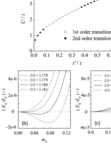
Figure 3: (a) Critical interaction strength at the paramagnetic-antiferromagnetic transition as a function of $t^{\prime}/t$. (b) The energy of the antiferromagnetic state $E_{{\rm N}}$ as a function of the magnetic moment $m_{{\rm N}}$ for different repulsion strength for $t^{\prime}/t=0.05$, with $m_{{\rm N}}=0$ at the transition. (c) $E_{{\rm N}}$ for $t^{\prime}/t=0.1$, with $m_{{\rm N}}\neq 0$ at the transition. The reference energy $E_{P}$ is the energy of the paramagnetic state for $m_{{\rm N}}=0$.

The paramagnetic-antiferromagnetic transition was first found by Lin and Hirsch Lin87 . In later studies, it was recognized that this transition can be either a first-order or second-order transition depending on the hopping ratio $t^{\prime}/t$ Kondo95 ; Hofstetter98 . A narrow region of a metallic antiferromagnetic state may exist near the transition Yang99 ; Duffy97 ; Chitra99 . Our numerical results show that the second-order transition takes place not only in the region with $t^{\prime}/t\gtrsim 0.38$ Kondo95 ; Hofstetter98 , but also in the region with $t^{\prime}/t\lesssim 0.08$, as can be seen from the vanishing magnetic moment $m_{{\rm N}}$ of the antiferromagnetic state at the transition in Fig. 3. When $0.08\lesssim t^{\prime}/t\lesssim 0.38$, the magnetic moment $m_{{\rm N}}$ is finite at the transition, indicating that it is a first-order phase transition. Near the second-order paramagnetic-antiferromagnetic transition, there is a tiny region of metallic antiferromagnetic state; near the first order transition, the antiferromagnetic state is always an insulator.

Figure 4: The mean-field phase diagram of the $2d$-Hubbard model at half filling. AFI denotes antiferromagnetic insulator, AFM denotes antiferromagnetic metal, CAFI denotes collinear antiferromagnetic insulator, CAFM denotes collinear antiferromagnetic metal, and PM denotes paramagnetic metal.

By comparing energies of paramagnetic, antiferromagnetic, and CAF states, we have obtained the mean-field phase diagram of the $2d$-Hubbard model at half filling as shown in Fig. 4. These three phases meet at a tricritical point $(t^{\prime}=0.707t,U=4.01t)$. The paramagnetic state is always the ground state when the repulsion is small enough. When $0<t^{\prime}/t<0.707$, there is a transition between paramagnetic and antiferromagnetic phases at a critical repulsion, which can be seen from the energy comparison shown in Fig. 5(a). When $0<t^{\prime}/t\lesssim 0.08$ or $0.38\lesssim t^{\prime}/t<0.707$, it is a second order transition; when $0.08\lesssim t^{\prime}/t\lesssim 0.38$, it is a first-order transition, as shown in Fig. 3.

Figure 5: Comparison between CAF-state energy $E_{{\rm C}}$ and antiferromagnetic-state energy $E_{{\rm N}}$ for: (a) $t^{\prime}/t=0.65$, (b) $t^{\prime}/t=0.76$ and (c) $t^{\prime}/t=0.8$, where $E_{\rm P}$ is the paramagnetic-state energy.

In the region with $0.707<t^{\prime}/t<0.774$ and $U>U_{{\rm P}}$, CAF and antiferromagnetic states have close energies, and there is a reentrance from the CAF state to the antiferromagnetic state as can be seen from the energy comparison shown in Fig. 5(b). There is a transition between the metallic CAF and antiferromagnetic states at a critical repulsion $U_{{\rm N}}$ larger than $U_{{\rm P}}$. However the metallic antiferromagnetic region is very small. When the repulsion further increases, the antiferromagnetic state becomes insulating, and eventually a transition between insulating antiferromagnetic and CAF states takes place at another critical repulsion $U_{{\rm C}}$. The transitions between antiferromagnetic and CAF states at $U_{{\rm C}}$ and $U_{{\rm N}}$ are the first-order transitions, because antiferromagnetic and CAF order parameters are discontinuous. Since the parameters $U$, $t$ and $t^{\prime}$ are of the same order at these transitions, fluctuations may modify these phase boundaries. In the phase diagram in Ref. Tremblay08 , the antiferromagnetic and CAF phases are separated by a very small paramagnetic region in between. In Ref. Tocchio08 , the CAF-antiferromagnetic transition was found near $t^{\prime}/t\approx 0.78$ without reentrance. The detail of this transition needs to be resolved in future studies.

For $t^{\prime}/t>0.774$ and $U>U_{{\rm P}}$, the CAF state has always lower energy than the antiferromagnetic state, as shown in Fig. 5(c). In the metallic CAF state, the magnetic moment $m$ has a kink for $t^{\prime}/t\lesssim 0.84$ and a discontinuity for $t^{\prime}/t\gtrsim 0.84$, when the van Hove singularity is at the Fermi surface. The metal-insulator transition takes place inside the CAF state at repulsion $U_{\rm MI}$ where also the magnetic moment $m$ has a kink .

V Discussion and conclusion

The location of the CAF phase in the mean-field phase diagram is in qualitative agreement with those obtained in other approaches Imada01 ; Tocchio08 ; Tremblay08 . We would like to stress that the mean-field method is more accurate when the on-site repulsion is relatively small. It is inadequate for treating spin-liquid or superconducting states Imada01 ; Tocchio08 ; Tremblay08 ; Yokoyama06 due to strong correlation. Spin frustration can significantly change the magnetic excitations in the antiferromagnetic stateDelannoy09 . Beyond half filling, ferromagnetic state, incommensurate spin-density-wave state, and phase separation Igoshev10 between these states can also appear.

In conclusion, we studied the CAF state in a half-filled $2d$ Hubbard model with NN and NNN hoppings at zero temperature. We found that a metal-insulator transition takes place inside the CAF phase at a critical on-site repulsion $U_{\rm MI}$. In the metallic CAF state, there is a kink or discontinuity in the magnetic moment when the van Hove singularity is at the Fermi surface. At zero temperature, the CAF, antiferromagnetic, and paramagnetic states meet at a tricritical point $(t^{\prime}=0.707t,U=4.01t)$. There is a first-order CAF-antiferromagnetic phase transition, and a second-order CAF-paramagnetic phase transition. The mean-field phase diagram of the $2d$ Hubbard model is obtained.

References

- (1) J. Hubbard, Proc. R. Soc. London, Ser. A 276, 238, (1963).
- (2) H. Q. Lin and J. E. Hirsch, Phys. Rev. B 35, 3359 (1987).
- (3) H. Kondo and T. Moriya, J. Phys. Soc. Jpn. 65, 2559 (1996); H. Kondo and T. Moriya, ibid., 67, 234 (1998).
- (4) W. Hofstetter and D. Vollhardt, Ann. d. Physik 7, 48 (1998).
- (5) D. Duffy and A. Moreo, Phys. Rev. B 55, R676 (1997).
- (6) I. Yang, E. Lange, and G. Kotliar, Phys. Rev. B 61, 2521 (2000).
- (7) R. Chitra, and G. Kotliar, Phys. Rev. Lett. 83, 2386 (1999).
- (8) T. Kashima and M. Imada, J. Phys. Soc. Jpn. 70, 3052 (2001); H. Morita, S. Watanabe, and M. Imada, ibid. 71, 2109 (2002); T. Mizusaki and M. Imada Phys. Rev. B 74, 014421 (2006).
- (9) L. F. Tocchio, F. Becca, A. Parola, and S. Sorella, Phys. Rev. B 78, 041101(R) (2008).
- (10) A. H. Nevidomskyy, C. Scheiber, D. Senechal, and A. M. S. Tremblay, Phys. Rev. B 77, 064427 (2008); see also, S. R. Hassan, B. Davoudi, B. Kyung, and A. M. S. Tremblay, Phys. Rev. B 77, 094501 (2008).
- (11) P. Chandra, P. Coleman and A. I. Larkin, Phys. Rev. Lett. 64, 88 (1990).
- (12) Q. P. Li and R. Joynt, Phys. Rev. B. 49, 1632 (1994).
- (13) B. Valenzuela, M. A. H. Vozmediano, and F. Guinea, Phys. Rev. B 62, 11312 (2000).
- (14) A. Avella, F. Mancini, and R. Münzner, Phys. Rev. B 63, 245117 (2001).
- (15) H. Taniguchi, Y. Morita, and Y. Hatsugai, Phys. Rev. B 71 134417 (2005).
- (16) H.Yokoyama, M. Ogata, and Y. Tanaka, J. Phys. Soc. Jpn. 75, 114706 (2006); S. Onari, H. Yokoyama, and Y. Tanaka, Physcia C, 463-465, 120 (2007).
- (17) G. I. Japaridze, R. M. Noack, D. Baeriswyl, and L. Tincani, Phys. Rev. B 76, 115118 (2007).
- (18) R. Peters and T. Pruschke, New J. Phys. 11, 083022 (2009).
- (19) J.-Y. P. Delannoy, M. J. P. Gingras, P. C. W. Holdsworth, and A.-M. S. Tremblay, Phys. Rev. B 79, 235130 (2009).
- (20) P. A. Igoshev, M. A. Timirgazin, A. A. Katanin, A. K. Arzhnikov, and V. Yu. Irkhin, Phys. Rev. B 81, 094407 (2010).