High-spin intruder band in ¹⁰⁷In

Abstract

High-spin states in the neutron deficient nucleus ¹⁰⁷In were studied via the ⁵⁸Ni(⁵²Cr, 3p) reaction. In-beam $\gamma$ rays were measured using the JUROGAM detector array. A rotational cascade consisting of ten $\gamma$-ray transitions which decays to the 19/2⁺ level at 2.002 MeV was observed. The band exhibits the features typical for smooth terminating bands which also appear in rotational bands of heavier nuclei in the A$\sim$100 region. The results are compared with Total Routhian Surface and Cranked Nilsson-Strutinsky calculations.

I Introduction

The structure of nuclei close to ¹⁰⁰Sn has received increasing attention in recent years. Excited states of neutron deficient nuclei with Z$\sim$50 are expected to be predominantly of single-particle nature at low spin due to the presence of a spherical shell gap for protons. However, recent experimental and theoretical investigations have elucidated additional important excitation mechanisms, such as magnetic rotation magrot , and deformed rotational bands of dipole and quadrupole character exhibiting smooth band termination smooth1 ; sb109 ; Smooth-PR ; smooth-dipole ; sn108 ; Te110 . The diversity of excitation modes in these nuclei make them particularly interesting systems to study.

In the A$\sim$100 region, the observation of well-deformed structures are interpreted as being based on 1p-1h smooth-dipole ; Te110 and 2p-2h smooth1 ; Smooth-PR ; sb109 ; sn108 proton excitations across the Z=50 closed-shell gap and on the occupation of the intruder $h_{11/2}$ orbital. These studies have in particular high-lighted the so-called “smooth band termination” phenomenon, following alignment of the valence nucleons outside the ¹⁰⁰Sn doubly-magic core. In the previous studies, levels in ¹⁰⁷In were extended up to $I$= (33/2) at 6.893 MeV, the last member of a magnetic-dipole band structure in107_prc58 . A well deformed intruder structure has been observed earlier in ¹⁰⁷In (see Fig. 23 in Ref. Smooth-PR ), but its detailed analysis has not been published so far.

In order to further investigate the existence of well-deformed structures in the A$\approx$100 mass region, we have obtained new data on the high-spin states of ¹⁰⁷In. In the present work, a rotational band was observed, extending to high angular momentum ($>30\hbar$). It is connected with the low-lying yrast states via several $\gamma$-ray transitions.

A rotational-like level structure in ¹⁰⁷In has recently been reported in107_epja43 . Although some of the $\gamma$-ray transitions are identical to those observed in the present work, the results are generally not in agreement with the results obtained in the present work. The band was not observed to lower spin states and it was not connected to the lower-lying states in ¹⁰⁷In.

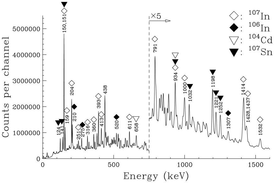
Figure 1: Total $\gamma-\gamma$ coincidence spectrum. Gamma-ray peak energies are labeled in keV for strong peaks. Previously known transitions in ¹⁰⁷In as well as those from the other principal evaporation residues, ¹⁰⁴Cd, ¹⁰⁶In, and ¹⁰⁷Sn are observed as indicated in the figure.

II Experimental details

The experiment was performed at the JYFL accelerator facility at the University of Jyväskylä, Finland. The ⁵²Cr ions, accelerated by the JYFL $K$ $=$ 130 MeV cyclotron to an energy of 187 MeV, were used to bombard a target consisting of two stacked self-supporting foils of isotopically enriched (99.8%) ⁵⁸Ni. The targets were of thickness 580 $\mu$g/cm² and 640 $\mu$g/cm². The average beam intensity was 4.4 particle-nA during 5 days of irradiation time. High-spin states in ¹⁰⁷In were populated by the fusion-evaporation reaction ⁵⁸Ni(⁵²Cr, 3p)¹⁰⁷In. Prompt $\gamma$-rays were detected at the target position by the JUROGAM $\gamma$-ray spectrometer consisting of 43 EUROGAM eurogam type escape-suppressed high-purity germanium detectors. In this configuration, JUROGAM had a total photopeak efficiency of about 4.2% at 1.3 MeV. Fig. 1 shows a total $\gamma-\gamma$ coincidence spectrum. Gamma-ray peaks of ¹⁰⁷In are observed as belonging to the strongest fusion-evaporation channel (3p). Other reaction channels such as ¹⁰⁴Cd (1$\alpha$2p), ¹⁰⁶In (3p1n), and ¹⁰⁷Sn (2p1n) are also observed clearly.

The fusion-evaporation products were separated in flight from the beam particles using the gas-filled recoil separator RITU ritu1 ; ritu2 and implanted into the two double-sided silicon strip detectors (DSSSD) of the GREAT great spectrometer. The GREAT spectrometer is a composite detector system containing, in addition to the DSSSDs, a multiwire proportional counter (MWPC), an array of 28 Si PIN photodiode detectors, and a segmented planar Ge detector. Each DSSSD has a total active area of 60$\times$40 mm² and a strip pitch of 1 mm in both directions yielding in total 4800 independent pixels. In this measurement, GREAT was used to filter the events such that recoils were separated and transported to the final focal plane of RITU.

The signals from all detectors were recorded independently and provided with an absolute “time stamp” with an accuracy of 10 ns using the total data readout (TDR) tdr acquisition system. Events associated with the recoil hitting DSSSD of GREAT and prompt $\gamma$ rays detected by JUROGAM were sorted offline using GRAIN analysis package GRAIN to store the recoil-gated multifold $\gamma$ coincidence data. In total 5.3$\times$10⁸ events were accumulated. The data were analyzed using the RADWARE data analysis software package radware . The multifold event data were sorted offline into an E_γ-E_γ correlation matrix and an E_γ-E_γ-E_γ cube. Based on single and double gating on the matrix and cube, respectively, coincidence relations between observed $\gamma$ rays were examined. Fig. 2 shows a level scheme constructed in the present study.

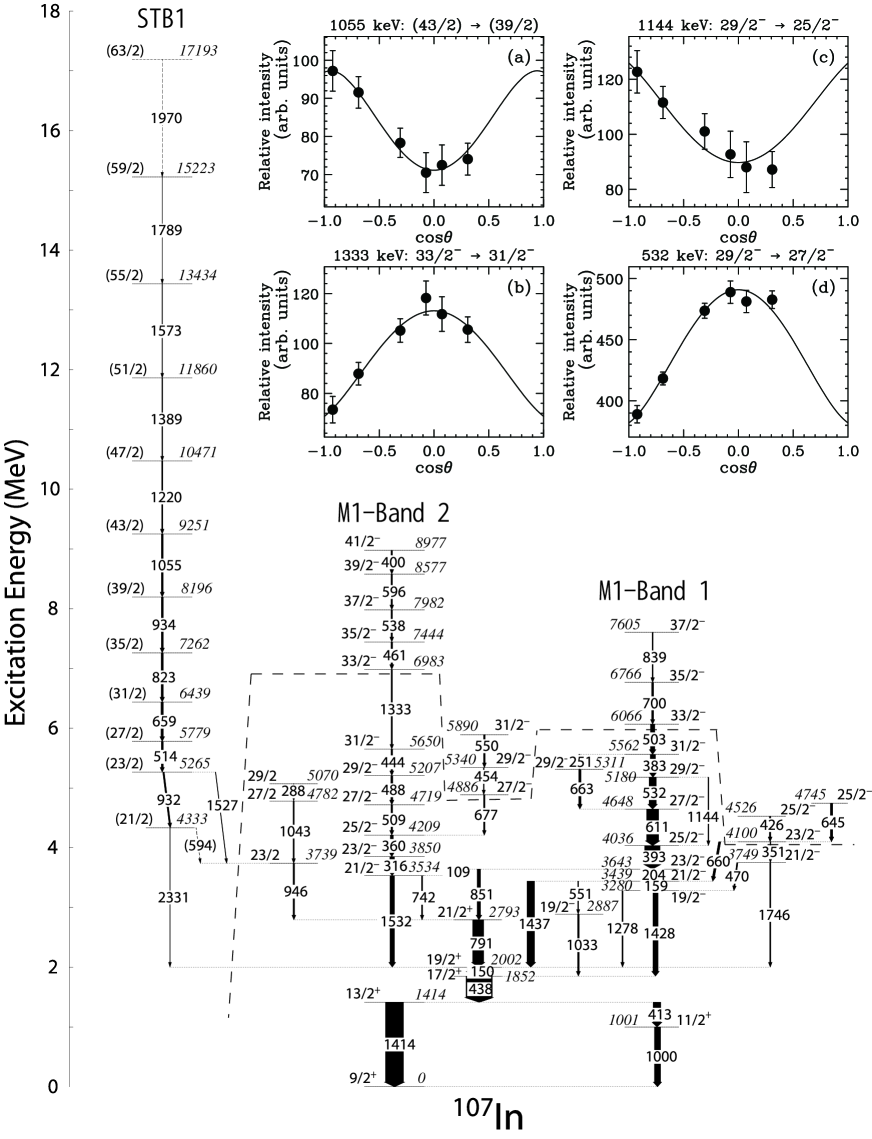
Figure 2: A level scheme of ¹⁰⁷In constructed in the present study. Transitions below dashed lines were previously identified in107_prc58 . Insets (a), (b), (c), (d) represent the typical angular distribution of $\gamma$ transitions observed with present setup. Solid lines are fitted curve of the angular distribution function W($\theta$).

In order to determine the $\gamma$-ray multipolarities, an angular distribution analysis was performed. The germanium detectors of the JUROGAM spectrometer were distributed over six angles relative to the beam direction with five detectors at 158^∘, ten at 134^∘, ten at 108^∘, five at 94^∘, five at 86^∘, and eight at 72^∘. Recoil gated coincidence matrices were sorted such that the energies of $\gamma$ rays detected at specified angles of JUROGAM, E_γ($\theta$), were incremented on one axis, while the energies of coincident $\gamma$ rays detected at any angles, E_γ(any), were incremented on the other axis. Six angular distribution matrices corresponding to the angles $\theta=158^{\circ},134^{\circ},94^{\circ},86^{\circ}$, and $72^{\circ}$ were created. Background-subtracted angle-dependent spectra were created by gating on transitions on the E_γ(any) of the matrices. Peak areas for a given coincident transition were measured and normalized by the number of detectors as well as efficiencies at each angle, then fitted to the angular distribution function W($\theta$) $=$ a₀(1 + a₂P₂(cos$\theta$) + a₄P₄(cos$\theta$)). In the case of stretched quadrupole (E2) transitions, a₂ and a₄ coefficients will have positive and small negative values, respectively, while those of pure stretched dipole (M1 or E1) transitions will be negative and zero values, respectively.

III Results

High-spin levels in ¹⁰⁷In were previously reported up to the ($I$ = 33/2) state at 6.983 MeV excitation energy in107_prc58 . The spin-parity of the ground state is 9/2⁺, arising from its $\pi g_{9/2}$ hole character. The 19/2⁺ state at 2.002 MeV and the 17/2⁺ state at 1.852 MeV have been reported to have isomeric character with half-lives of 0.6(2) and 1.7(3) ns, respectively in107_isomer . These lifetimes are long enough so that the $\gamma$-ray emission depopulating these states or lower-lying states which are fed via these states, on average occurs several cm downstream from the target. This affects the relative efficiency of detecting such $\gamma$ rays depending on the detector angle relative to the beam and hence their angular distribution. An attenuation of the alignment could also be affected by the level lifetimes. Indeed, the angular distributions of transitions below the state at 1.852 MeV were observed to be isotropic. However, the angular distribution of the 150 keV transition below the 0.6 ns isomer at 2.002 MeV was not isotropic. This is consistent with the fact that the half-life of the isomer is shorter than that of the 1.852 MeV level. The half-lives of these two isomers could not be confirmed in this analysis since the experimental setup was not sensitive for such short lifetimes.

Table 1: Gamma rays assigned to ¹⁰⁷In

$E_{\gamma}$a	$I^{(rel.)}{\gamma}^{b}$	$E_{i}$c	$a_{2}$	$a_{4}$	$J^{\pi}_{i}$	$\rightarrow$	$J^{\pi}_{f}$
(keV)		(keV)
109.3	14(2)	3643	$-0.23(17)$	$0.24(23)$	$23/2^{-}$	$\rightarrow$	$21/2^{-}$
149.8	768(48)	2002	$-0.260(15)$	$0.025(22)$	$19/2^{+}$	$\rightarrow$	$17/2^{+}$
158.6	183(12)	3439	$-0.266(16)$	$0.003(22)$	$21/2^{-}$	$\rightarrow$	$19/2^{-}$
204.0	437(26)	3643	$-0.280(15)$	$0.065(22)$	$23/2^{-}$	$\rightarrow$	$21/2^{-}$
251.2	50(3)	5562	$-0.242(47)$	$0.132(69)$	$31/2^{-}$	$\rightarrow$	$29/2^{-}$
288.4	17(2)	5070	$-0.36(12)$	$0.10(17)$	29/2	$\rightarrow$	27/2
315.6	175(12)	3850	$-0.224(21)$	$0.025(31)$	$23/2^{-}$	$\rightarrow$	$21/2^{-}$
351.4	33(3)	4100	$-0.30(18)$	$-0.08(28)$	$23/2^{-}$	$\rightarrow$	$21/2^{-}$
359.6	115(8)	4209	$-0.236(27)$	$0.010(40)$	$25/2^{-}$	$\rightarrow$	$23/2^{-}$
382.9	194(12)	5562	$-0.272(14)$	$0.070(21)$	$31/2^{-}$	$\rightarrow$	$29/2^{-}$
393.0	580(36)	4036	$-0.219(25)$	$0.024(37)$	$25/2^{-}$	$\rightarrow$	$23/2^{-}$
400.2	53(4)	8977	$-0.244(31)$	$0.011(50)$	$41/2^{-}$	$\rightarrow$	$39/2^{-}$
413.2	289(22)	1414	$-0.101(62)$	$0.117(88)$	$13/2^{+}$	$\rightarrow$	$11/2^{+}$
426.3	59(6)	4526	$-0.484(51)$	$-0.004(74)$	$25/2^{-}$	$\rightarrow$	$23/2^{-}$
438.2	1000(60)	1852	$0.071(31)$	$0.068(45)$	$17/2^{+}$	$\rightarrow$	$13/2^{+}$
443.6	62(5)	5654	$-0.383(29)$	$0.154(43)$	$31/2^{-}$	$\rightarrow$	$29/2^{-}$
454.4	33(3)	5340	$-0.218(40)$	$0.076(59)$	$29/2^{-}$	$\rightarrow$	$27/2^{-}$
460.5	63(4)	7444	$-0.206(2)$	$0.056(2)$	$35/2^{-}$	$\rightarrow$	$33/2^{-}$
469.6	48(6)	3749	$-0.094(38)$	$0.030(55)$	$21/2^{-}$	$\rightarrow$	$19/2^{-}$
488.2	75(6)	5207	$-0.204(38)$	$-0.025(56)$	$29/2^{-}$	$\rightarrow$	$27/2^{-}$
503.4	167(10)	6066	$-0.237(52)$	$-0.053(78)$	$33/2^{-}$	$\rightarrow$	$31/2^{-}$
509.3	69(6)	4719	$-0.238(41)$	$0.140(60)$	$27/2^{-}$	$\rightarrow$	$25/2^{-}$
514.3	75(8)	5779	$0.276(59)$	$-0.109(87)$	(27/2)	$\rightarrow$	(23/2)
532.1	276(18)	5180	$-0.180(1)$	$0.039(2)$	$29/2^{-}$	$\rightarrow$	$27/2^{-}$
537.7	54(4)	7982	$-0.286(34)$	$0.188(50)$	$37/2^{-}$	$\rightarrow$	$35/2^{-}$
550.1	58(5)	5890	$-0.242(33)$	$0.138(48)$	$31/2^{-}$	$\rightarrow$	$29/2^{-}$
551.1	31(4)	3439			$21/2^{-}$	$\rightarrow$	$19/2^{-}$
593.8	5(3)	4333			21/2	$\rightarrow$	23/2
595.5	56(4)	8577	$-0.325(14)$	$0.025(21)$	$39/2^{-}$	$\rightarrow$	$37/2^{-}$
611.3	463(28)	4648	$-0.131(31)$	$-0.017(45)$	$27/2^{-}$	$\rightarrow$	$25/2^{-}$
644.5	87(8)	4745	$-0.187(24)$	$-0.063(35)$	$25/2^{-}$	$\rightarrow$	$23/2^{-}$
659.0	90(8)	6439	$0.278(36)$	$-0.126(53)$	(31/2)	$\rightarrow$	(27/2)
659.7	83(10)	4100			$23/2^{-}$	$\rightarrow$	$21/2^{-}$
663.2	89(8)	5311	$-0.225(35)$	$0.048(55)$	$29/2^{-}$	$\rightarrow$	$27/2^{-}$
676.6	52(5)	4886	$-0.03(10)$	$0.11(16)$	$27/2^{-}$	$\rightarrow$	$25/2^{-}$
700.4	73(6)	6766	$-0.291(60)$	$-0.067(93)$	$35/2^{-}$	$\rightarrow$	$33/2^{-}$
741.5	45(4)	3534	$0.243(61)$	$-0.155(93)$	$21/2^{-}$	$\rightarrow$	$21/2^{+}$
791.0	419(28)	2793	$-0.122(31)$	$0.023(52)$	$21/2^{+}$	$\rightarrow$	$19/2^{+}$
823.1	81(10)	7262	$0.242(17)$	$-0.124(68)$	(35/2)	$\rightarrow$	(31/2)
838.8	45(4)	7605	$-0.179(34)$	$0.040(52)$	$37/2^{-}$	$\rightarrow$	$35/2^{-}$
850.6	133(10)	3643	$-0.296(4)$	$0.038(6)$	$23/2^{-}$	$\rightarrow$	$21/2^{+}$
932.4	58(12)	5265			(23/2)	$\rightarrow$	21/2
934.0	75(12)	8196	$0.253(54)$	$-0.183(81)$	(39/2)	$\rightarrow$	(35/2)
945.8	57(8)	3739	$-0.16(11)$	$0.19(16)$	23/2	$\rightarrow$	$21/2^{+}$
1000.4	234(18)	1001	$-0.050(36)$	$-0.076(53)$	$11/2^{+}$	$\rightarrow$	$9/2^{+}$
1032.8	66(14)	2887	$0.16(10)$	$0.13(16)$	$19/2^{-}$	$\rightarrow$	$17/2^{+}$
1042.8	43(6)	4782	$0.148(81)$	$-0.13(13)$	27/2	$\rightarrow$	23/2
1055.0	68(12)	9251	$0.241(24)$	$-0.089(37)$	(43/2)	$\rightarrow$	(39/2)
1143.8	35(5)	5180	$0.248(57)$	$-0.038(85)$	$29/2^{-}$	$\rightarrow$	$25/2^{-}$
1220.1	49(12)	10471	$0.297(41)$	$-0.045(61)$	(47/2)	$\rightarrow$	(43/2)
1278.0	45(5)	3280	$0.327(39)$	$-0.067(55)$	$19/2^{-}$	$\rightarrow$	$19/2^{+}$
1333.2	50(4)	6983	$-0.319(29)$	$0.059(44)$	$33/2^{-}$	$\rightarrow$	$31/2^{-}$
1389.0	30(8)	11860	$0.263(29)$	$0.028(45)$	(51/2)	$\rightarrow$	(47/2)
1414.0	690(60)	1414	$0.047(29)$	$0.004(43)$	$13/2^{+}$	$\rightarrow$	$9/2^{+}$
1428.1	199(18)	3280	$-0.137(25)$	$0.084(38)$	$19/2^{-}$	$\rightarrow$	$17/2^{+}$
1437.4	290(18)	3439	$-0.207(22)$	$0.049(35)$	$21/2^{-}$	$\rightarrow$	$19/2^{+}$
1527.0	18(4)	5265			(23/2)	$\rightarrow$	23/2
1532.3	172(14)	3534	$-0.337(10)$	$-0.036(15)$	$21/2^{-}$	$\rightarrow$	$19/2^{+}$
1573.3	20(2)	13434	$0.29(17)$	$-0.06(27)$	(55/2)	$\rightarrow$	(51/2)
1746.5	48(6)	3749	$-0.322(67)$	$0.026(96)$	$21/2^{-}$	$\rightarrow$	$19/2^{+}$
1789.4	9(2)	15223			(59/2)	$\rightarrow$	(55/2)
1969.7	3(1)	17193			(63/2)	$\rightarrow$	(59/2)
2330.5	17(2)	4333	$0.23(9)$	$0.24(13)$	21/2	$\rightarrow$	$19/2^{+}$
aTransition energies accurate to within $\pm 0.5\,$keV. bIntensities are normalized to 1000 for the 438 keV $\gamma$ transition. cExcitation energies of initial states of $\gamma$ transitions.

Figure 3: Gamma-ray energy spectrum gated by the 1428 and 159 keV transitions. The inset enlarges the region between 600 keV and 1 MeV.

Figure 4: Gamma-ray energy spectrum gated by the 1532 and 316 keV transitions. The inset enlarges the region between 350 and 650 keV.

Above the isomeric 19/2⁺ level, high-energy $\gamma$-ray transitions of $\sim$1.5 MeV connect to the 19/2^- level at 3.280 MeV and 21/2^- level at 3.534 MeV. These levels are suggested to be based on the $\pi$g${}_{9/2}^{-1}\otimes\nu$(h_11/2,g_7/2) configuration, i.e. a neutron excitation between the g_7/2 and h_11/2 sub-shells. The two sequences of magnetic dipole transitions have previously been observed to connect negative parity states up to 33/2^(-) in107_prc58 .

Gamma-ray coincidence relations of previously reported transitions in107_prc58 were confirmed as shown in the right part of partial level scheme in Fig. 2. Table LABEL:gamma_table summarizes $\gamma$ rays assigned to ¹⁰⁷In. The relative intensity of each $\gamma$ transition was extracted by fitting the $\gamma$-$\gamma$ correlation matrix by taking into account the $\gamma$-ray intensities of feeding transitions, branching ratio, and conversion coefficient of the lower transitions using the ESCL8R program in the RADWARE software package radware .

By gating on the E_γ-E_γ matrix and the E_γ-E_γ-E_γ cube, coincidence relations between known $\gamma$ rays and newly observed $\gamma$ rays were examined. Fig. 3 shows a $\gamma$ ray energy spectrum obtained by double gating in the cube on the 1428 and 159 keV transitions which are members of one of the sequences of magnetic dipole transitions (M1-band 1). Gamma-ray transitions up to the 33/2^- level at 6.066 MeV (see Fig. 2) were confirmed and two new transitions, 700 and 839 keV, were placed above this level. These two transitions also have M1 character as shown in table LABEL:gamma_table.

Fig. 4 shows a spectrum obtained by double-gating in the cube on the 1532 and 316 keV transitions which are members of another M1 sequence (M1-band 2). Gamma-ray transitions up to the 33/2^- level at 6.983 MeV were confirmed and in addition four $\gamma$-ray transitions were observed in coincidence with the sequence. Based on the angular distribution analysis, the multipolarities of these four transitions were assigned as M1 and accordingly the spins and parities of the four levels above the 33/2^- level were assigned up to the 41/2^- level at 8.977 MeV.

Figure 5: Sum of $\gamma$-ray energy spectra created by double-gating on the in-band transitions of the rotational band (STB1). The inset enlarges the region between 1.45 and 2.5 MeV.

Figure 6: Gamma-ray energy spectrum gated by the 2331 keV linking transition from the $\gamma-\gamma$ matrix.

Figure 7: Gamma-ray energy spectrum created by gating on the in-band transition of the rotational band in one axis, and the 946, 791, 150, 438, 413, 1000, and 1414 keV transitions in the other axis of $\gamma\gamma\gamma$ cube. The insets enlarge the regions from 0.5 MeV to 0.7 MeV, and from 1.45 MeV to 1.65 MeV, respectively.

In addition to the above mentioned M1 transitions, a rotational $\gamma$-ray cascade (STB1) consisting of the 514, 659, 823, 934, 1055, 1220, 1389, 1573, and 1789 keV transitions was observed by gating on the E_γ-E_γ matrix as shown in Fig. 2 and 5. A 1970 keV transition was tentatively placed on top of the band. The 934 keV transition has a larger intensity than the other neighboring in-band transitions, 823 and 1055 keV since it is a self-coincident doublet decomposed of a 932 keV and a 934 keV transition. Based on the intensity balance of the in-band transitions, a rotational band structure was assigned as shown in the left part of Fig. 2. In addition, the 2331 keV $\gamma$ ray is observed to be in coincidence with the assigned in-band transitions as well as the low-lying transitions, 150, 438, 413, and 1414 keV (see Fig. 6). Since this $\gamma$ ray is strongly in coincidence with the lowest-lying member of the band, as well as with the 932 keV-934 keV doublet, the decay path of the band is formed to precede the cascade of 932 and 2331 keV transitions to the 19/2⁺ state at 2.002 MeV as shown in the level scheme. Note that the intensity of the 932 keV transition in Table LABEL:gamma_table is larger than the sum of the 2331 keV and 594 keV intensities. Our interpretation is that there might be several weak unidentified $\gamma$ transitions decaying from the 4.333 MeV level carrying the intensity not accounted for. For example, in the double-gated spectrum on the in-band transitions (Fig. 5), a peak appeared at 1033 keV. This indicates the presence of a linking transition from the 4.333 MeV level to the 2.887 MeV level. However, any such $\gamma$ transitions were not observed due to the low statistics.

There is another decay path of the band via the 1527 keV transition from the 5.265 MeV state to the 3.739 MeV state. Fig. 7 shows a $\gamma$-ray energy spectrum created by gating on the in-band transitions of STB1 on one axis, and the 946, 791, 150, 438, 413, 1000, and 1414 keV transitions on the other axis of the $\gamma\gamma\gamma$ cube. As shown in the figure, the 594 and 1527 keV transitions are coincident with the in-band transitions above 5.265 MeV level as well as transitions below 3.739 MeV level. These 594 and 1527 keV transitions correspond to the links from 4.333 to 3.739 MeV level and from 5.265 to 3.739 MeV level, respectively. These two decay paths establish the excitation energy of the observed lowest level of the band to be 5.265 MeV.

In Fig. 5, the 1573 keV peak appears stronger than the 1527 keV peak compared to the relative intensities presented in Table LABEL:gamma_table. Since the spectrum shown in Fig. 5 was created by double-gating on the in-band transitions of STB1 including the 932, 934 keV doublet, it contains double-gating between the 932 keV $\gamma$ ray and other $\gamma$ rays of STB1. Therefore, the counts in the 1573 keV peak in Fig. 5 was artificially increased relative to that of the 1527 keV transition.

The excitation energies of the yrast levels and the levels in the STB1 were plotted as a function of spin in the upper panel of Fig. 8. In the lower panel of Fig. 8, relative intensities of the yrast transitions and the in-band transitions are plotted. One can see that the M1-band 1 becomes yrast above spin 10 $\hbar$, and that the STB1 becomes yrast around spin 18 $\hbar$. The intensity profiles are consistent with the trend of yrast sequences formed by M1-band 1 and STB1.

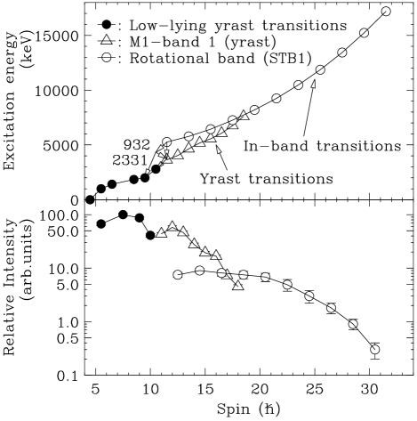
Figure 8: Excitation energies of the yrast levels and the levels in the rotational band as a function of spin (upper panel). Relative intensities of yrast $\gamma$ transitions and those of the band are plotted as a function of spin in the lower panel.

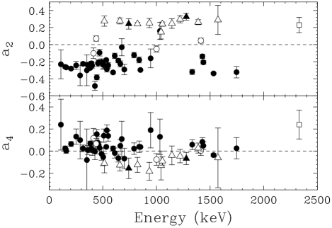
Figure 9: A plot of a₂ and a₄ coefficients of $\gamma$-ray angular distributions, W($\theta$)=a₀(1+a₂P₂(cos$\theta$)+a₄P₄(cos$\theta$)), as a function of $\gamma$-ray energy. Here, $\theta$ is the emission angle of $\gamma$ rays relative to the beam axis and P_n(cos$\theta$) are the Legendre polynomials. Filled circles and filled triangles correspond to the angular distribution of known M1 and $\Delta$I=0 E1 transitions, respectively. Open circles indicate those of the transitions below the isomeric state at 1.852 MeV. Open triangles correspond to those of the identified in-band transitions as well as known E2 transition (1144 keV). The open square is for the case of the 2331 keV linking transition.

Multipolarity assignments for the observed $\gamma$-ray transitions were deduced from the angular distribution analysis. Fig. 9 displays the a₂ and a₄ coefficients of the $\gamma$-ray angular distribution function plotted as a function of the $\gamma$-ray energy. Filled circles and filled triangles correspond to the angular distribution of known M1 transitions and $\Delta$I=0 E1 transitions, respectively, which agree with theoretical estimates. Open circles are for the $\gamma$-ray transitions decaying from the isomeric state at 1.852 MeV and they show small values as expected. Open triangles correspond to those of the newly identified cascade transitions which are consistent with a stretched E2 character.

Figure 10: $\chi^{2}$ vs tan${}^{-1}\delta$ curves for the 2331 keV transition in ¹⁰⁷In. The parameters indicated were used to compute the curves.

As shown in Fig. 9, the angular distribution of the 2331 keV linking transition (open square) does not clearly determine its multipolarity due to the low statistics. The positive a₂ value may indicate that it contains a quadrupole component in its multipolarity and the positive a₄ may reflect a mixed transition. In order to try and resolve this ambiguity, the mixing ratio that satisfies the 99.9$\%$ confidence limit test in $\chi^{2}$ (defined as in equatoin (1) ang_delta ) is plotted as a function of tan${}^{-1}\delta$ in Fig. 10. Three different hypotheses were tested, 19/2$\rightarrow$19/2, 21/2$\rightarrow$19/2, and 23/2$\rightarrow$19/2.

$$\chi^{2}=\frac{[a_{2}-a_{2}(cal)]^{2}}{3(\Delta a_{2})^{2}}+\frac{[a_{4}-a_{4}(cal)]^{2}}{3(\Delta a_{4})^{2}}$$ (1)

As indicated in Fig. 10, a parameter ’$\sigma$/J’ is used to implement the initial alignment, where a Gaussian distribution for the magnetic substates is assumed and $\sigma$ and J denote the width and the spin, respectively. In the calculation, a ratio $\sigma$/J = 0.1 was assumed. The $\chi^{2}$ result suggests a mixed E2/M1 or M2/E1 transition, 21/2$\rightarrow$19/2⁺ with a mixing ratio of 0.23. Since Weisskopf estimate of lifetimes for a 2331 keV $\gamma$ ray are 0.4 ps for an E2 and 29 ps for an M2 transition, respectively, both cases are short enough for prompt $\gamma$ coincidence and therefore the parity of the 4.333 MeV state was not determined. Since the decay-out 932 keV $\gamma$-ray transition in cascade with the linking transition is close in energy to the 934 keV in-band transition, its multipolarity was not firmly identified. The statistics of another 1527 keV linking transition were too low to perform angular distribution analysis in order to establish the multipolarity. Under the assumption that a dipole transition connects the lowest level of the band with the 4.333 MeV level, the spin of the band was assigned as starting with (23/2) as shown in Fig. 2.

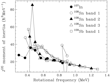
Figure 11: Experimentally deduced dynamical moments of inertia J⁽²⁾ in ¹⁰⁷In, ¹⁰⁸Sn, and ¹⁰⁹Sb. The data on ¹⁰⁷In is from the present work.

IV Discussion

In this mass region, the presence of rotational bands has been reported previously in the N$=$58 isotones, ¹⁰⁵Ag, ¹⁰⁶Cd, ¹⁰⁸Sn, ¹⁰⁹Sb, ¹¹⁰Te, and ¹¹¹I ag105 ; cd106 ; sn108 ; sb109 ; bob_prl ; sb109_2 ; Te110 ; i111 . Among them, rotational bands exhibiting a character of smooth band termination appeared only in ¹⁰⁸Sn, ¹⁰⁹Sb, and ¹¹⁰Te.

In Fig. 11, deduced dynamical moments of inertia J⁽²⁾ are shown as a function of rotational frequency. Here, the rotational frequency ($\omega$) and the dynamical moment of inertia J⁽²⁾ are deduced from the experimental data (E_γ) using the formulae,

$$\hbar\omega=\frac{dE}{d{\rm I}}\approx\frac{E_{\gamma}}{2}$$ (2)

and

$${\rm J}^{(2)}=\frac{d{\rm I}}{d\omega}\approx\frac{4}{\Delta{\rm E}_{\gamma}},$$ (3)

respectively. In addition to the band in ¹⁰⁷In, also the bands in ¹⁰⁸Sn sn108 , and ¹⁰⁹Sb sb109_2 are shown, which have positive parity for the neutron configuration according to the assignments based on the cranked Nilsson-Strutinsky calculations AR-95 . In general, all J⁽²⁾ values show the smooth decrease with increasing rotational frequency which is characteristic for smooth band termination in systems with weak pairing AR-95 ; Smooth-PR . This feature is disturbed only at the top of the band 1 in ¹⁰⁸Sn. The J⁽²⁾ values of ¹⁰⁷In show very close similarity with those in bands 2 and 3 of ¹⁰⁸Sn, while those in band 1 of ¹⁰⁸Sn and band 1 of ¹⁰⁹Sb are also very similar. This suggests that the structure of the band in ¹⁰⁷In is similar to that of bands 2 and 3 in ¹⁰⁸Sn. Bands 2 and 3 of ¹⁰⁸Sn were interpreted to be signature partner bands with the proton configuration of $\pi[$g${}_{9/2}^{-2}\otimes($g${}_{7/2}h_{11/2})]$ sn108 ; sn108_2 . On the other hand, band 1 of ¹⁰⁸Sn and ¹⁰⁹Sb were understood to have configurations of $\pi[$g${}_{9/2}^{-2}\otimes$g${}_{7/2}^{2}]$ and $\pi[$g${}_{9/2}^{-2}\otimes$g${}_{7/2}^{2}h_{11/2}]$, respectively. The hump observed in the J⁽²⁾ plot for band 1 of ¹⁰⁸Sn and ¹⁰⁹Sb, appearing at $\sim$0.55 MeV, was interpreted as due to the alignment of g_7/2 protons based on cranked Woods-Saxon calculations sn108_2 . These results indicate that deformation-driving down-sloping $\pi$g_7/2 and $\pi$h_11/2 orbitals and, especially, the holes in the $\pi g_{9/2}$ extruder orbitals play an important role to create the rotational band structures which undergo smooth band termination in this mass region AR-95 . In the case of ¹⁰⁷In, possible configurations of the observed band (STB1) would be $\pi[$g${}_{9/2}^{-2}\otimes$g${}_{7/2}]$ or $\pi[$g${}_{9/2}^{-2}\otimes$h${}_{11/2}]$ generated by removing one proton from ¹⁰⁸Sn.

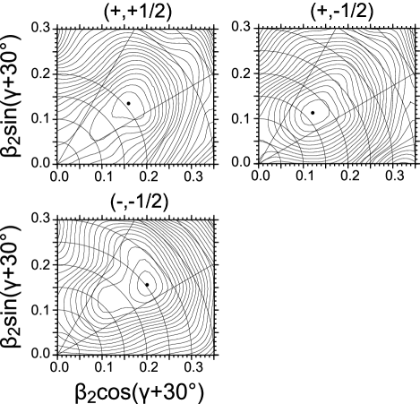
Figure 12: Calculated total Routhian surfaces (TRS) at a rotational frequency of 0.75 MeV. The lowest positive-parity configurations with signature +1/2 and -1/2 are shown in the left and right upper panels, respectively, while the lowest negative-parity configuration with signature -1/2 is plotted on the lower left panel.

Cranked Strutinsky calculations based on the Woods-Saxon (WS) WoodsSaxon and Nilsson (CNS) AR-95 ; Smooth-PR potentials were performed in order to interpret the structure of the observed rotational band (STB1). In the former total Routhian Surface (TRS) calculations, pairing correlations were taken into account by means of a seniority and double stretched quadrupole pairing force pairing . Approximate particle number projection was performed via the Lipkin-Nogami method LipkinNogami1 ; LipkinNogami2 . Each quasiparticle configuration was blocked self-consistently. The energy in the rotating frame of reference was minimized with respect to the deformation parameters $\beta_{2},\beta_{4}$ and $\gamma$. Deformed minima in the total Routhian surfaces (TRS) were found at ($\beta_{2},\gamma$) $\sim$ ($0.20,10^{\circ}$) for both signatures at positive parity ($\pi$,$\alpha$)$=$(+,$\pm$1/2) and at ($\beta_{2},\gamma$) $\sim$ ($0.25,8^{\circ}$) for the negative parity, negative signature configuration ($-$,$-$1/2) as shown in Fig. 12. The structure of the experimentally observed rotational band (STB1) in ¹⁰⁷In is likely to correspond to one of these configurations.

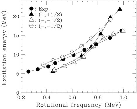
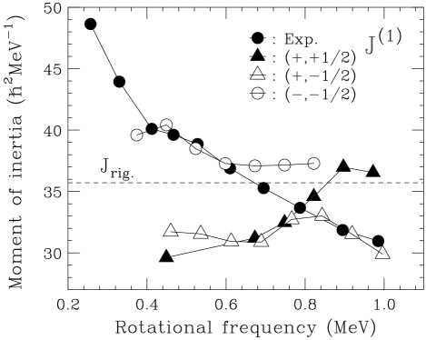
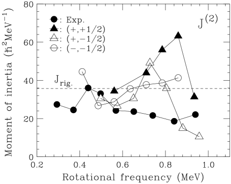
Figure 13: Comparison of experimental and calculated excitation energies, J⁽¹⁾ and J⁽²⁾ moments of inertia as a function of rotational frequency. The highest-frequency data point, which is originated from the tentatively assigned 1970 keV transition, is also included in the plot. Theoretical values were obtained by TRS calculations. The dashed line marks the rigid-body moment of inertia for a deformation parameter $\beta_{2}=$0.25.

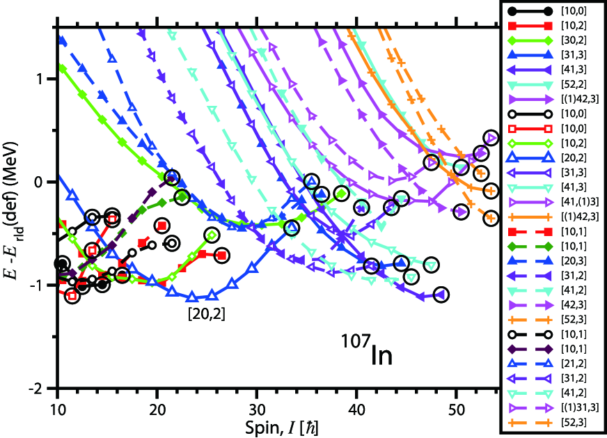
Figure 14: (Color online) Calculated energies of the configurations forming the yrast line in four combinations of parity and signature shown relative to rigid rotor reference. Large open circles indicate terminating and aligned states. Solid and dashed lines are used for positive and negative parity states, respectively. Solid and open symbols are used for the signatures $\alpha=+1/2$ and $\alpha=-1/2$, respectively. Configuration labels are shown in the legend.

Excitation energies, kinematic (J⁽¹⁾) and dynamic (J⁽²⁾) moments of inertia obtained from the TRS calculations are compared with experimental values in Fig. 13. In order to deduce the experimental J⁽¹⁾-moment of inertia, we have assumed the spin of the lowest level of the band to be 23/2. The TRS calculation shows that the configuration of positive parity with negative signature $(+,-1/2)$ is lowest in energy among the predicted configurations in the frequency range of interest. However, as can be seen in Fig. 13, J⁽¹⁾ and J⁽²⁾ moments of inertia for $(+,\pm 1/2)$ configurations show quite different behavior comparing with the experimental values. On the other hand, the configuration with $(-,-1/2)$ is in better agreement with the experimental properties except for the high frequency region. However, it is quite likely that the TRS calculations overestimate the role of pairing at high spin and this leads to observed discrepancies between experiment and calculations.

In the CNS AR-95 ; Smooth-PR calculations, the pairing is neglected and thus the results are expected to be realistic only at high spin, I$\geq$15$\hbar$. In general, a very good agreement Smooth-PR between the CNS calculations and observed high-spin bands in this mass region has been obtained with the $\kappa$- and $\mu$-values from Ref. par and these are the values which are used also in the present study. The calculations in the current analysis are performed using the CNS version of Ref. CR.06 , so that not only the relative energies between the bands but also the absolute energy scale can be compared. The single-particle configurations are defined by the occupation of low- and high-$j$ orbitals. The total energy of each configuration is minimized at each spin in the $(\varepsilon_{2},\varepsilon_{4},\gamma)$ deformation plane. Standard CNS labeling of each configuration is used. This shorthand notation is based on the number of particles in different $j$ shells for each configuration. The $j$ shells are pure only if the shape is spherical. Thus, in general the labeling refers to the dominant shell only, while the wave functions also contain components from other $N$ and $j$ shells. Relative to a closed ¹⁰⁰Sn core, a shorthand configuration label $[(p_{1})p_{2}p_{3},(n_{1})n_{2}]$ can be written as Smooth-PR

$$[(p_{1})p_{2}p_{3},(n_{1})n_{2}] = \pi(N=3)^{-p_{1}}(g_{9/2})^{p_{2}}(h_{11/2})^{p_{3}}$$ (4)

$$\otimes\,\,\nu(N=3)^{-n_{1}}(h_{11/2})^{n_{2}}$$

with the remaining particles (protons/neutrons) outside the core located in the mixed $(d_{5/2}\,g_{7/2})$ orbitals. The label $p_{1}$ ($n_{1}$) is dropped if no holes are generated in the $N=3$ proton (neutron) shell.

The results of the calculations are shown in Fig. 14. One can see that the [20,2] configuration dominates the yrast line in the spin range $I=20-31\hbar$. This configuration is therefore the most likely counterpart for the observed decoupled $\Delta I=2$ band. Fig. 15 compares the experimental band with the results of the calculations. Fig. 15a shows the experimental band for three different spin assignments $I_{0}$ for the lowest state in the band. Fig. 15b displays the configurations which can be possible counterparts of the experimental band. In Fig. 15a,b, the $y$ axis denotes the energy with the rotating liquid drop (rld) energy CR.06 subtracted. The energy difference between the predictions and observations is plotted in Fig. 15c. In the ideal case when the transition energies will be predicted correctly by the calculations for each transition in the band, the curve of the band in Fig. 15c will have a constant energy difference for all states of a given configuration, i.e. it will be horizontal. Furthermore, if the absolute energy is predicted correctly, this difference should be zero with the experience CR.06 that the difference will generally be smaller than one MeV, i.e. the absolute energy at high spin can be described with a similar accuracy as ground state masses. One can see that reasonable agreement between theory and experiment is obtained when the [20,2] configuration is assigned to the band; the deviation from the horizontal line in Fig. 15c of $\sim 1$ MeV is at the upper limit of the typical discrepancies between theory and experiment. For this configuration assignment, the observed band in ¹⁰⁷In is one transition short of termination. Further support for this configuration assignment comes from the analysis of the configurations of the smooth terminating bands in the $N=58$ isotones (see Fig. 23 in Ref.  Smooth-PR ). In ¹⁰⁸Sn, the yrast line in the spin range $I=20-28\hbar$ is dominated by the [20,2] configuration. This is exactly the same configuration (in terms of shorthand notation) as we assign to the $\Delta I=2$ band in ¹⁰⁷In. The difference between the [20,2] configurations in these two nuclei is related to an occupation of the extra $(d_{5/2}\,$g${}_{7/2})$ proton in ¹⁰⁸Sn. Note also that this configuration assignment fits exactly into the systematics of the configurations of smooth terminating bands observed in this mass region (see Fig. 20 and 23 in Ref. Smooth-PR ). Indeed, according to this figure, the present signature $\alpha=-1/2$ [20,2] band is predicted to be the most favored smooth terminating band in ¹⁰⁷In.

The evolution of the potential energy surfaces for the [20,2] configuration is shown in Fig. 16. This configuration displays typical features of smooth band termination gradually evolving from near-prolate shape at low spin up to a non-collective oblate shape at the terminating state with $I^{\pi}=67/2^{+}$. These energy surfaces are very regular thus showing no disturbances, neither from mixing with aligned states within the same configuration (see Ref. Smooth-PR for more details of such mechanism) nor from mixing with other collective configurations. This is a consequence of the fact that the nuclear system attempts to avoid a high level density in the vicinity of the Fermi level by a gradual adjustment of the equilibrium deformation with increasing spin Smooth-PR .

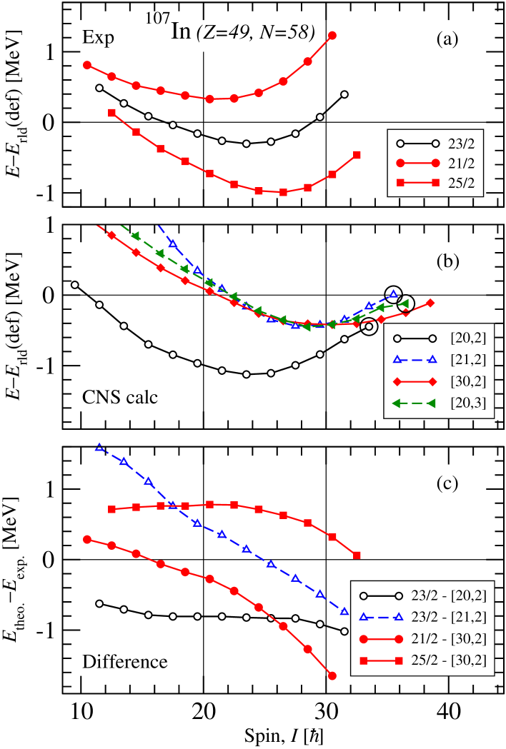
Figure 15: (Color online) Comparison between the experimentally observed $\Delta I=2$ rotational band (STB1) and the CNS predictions for selected configurations. The top panel shows the experimental band with different spin assignments $I_{0}$ for the lowest observed state. The middle panel shows the chosen predicted configurations. The bottom panel plots the energy difference between the predictions and observations.

Taking into account the uncertainty of spin-parity definition of the experimental $\Delta I=2$ band, one can consider also alternative configuration assignments. These are the [30,2], [20,3] and [21,2] configurations (Fig. 14). The [30,2] configuration involves an additional excitation from the proton $g_{9/2}$ subshell, while the [20,3] ([21,2]) configurations are built from the [20,2] configuration by moving the neutron from $(d_{5/2}\,g_{7/2})$ into $h_{11/2}$ (by moving the proton from $(d_{5/2}\,g_{7/2})$ into $h_{11/2}$). These changes require additional energy, and thus these configurations are less energetically favored than [20,2] (Figs. 14 and 15b). In addition, the spin of the lowest state in the band has to be changed either to $21/2$ or to $25/2$ if either the [30,2] or [20,3] configurations is to be assigned to the experimental band. Note that the calculated energies for the [20,3] and [30,2] configurations are similar (Fig. 15b). Thus, the [20,3] configuration is not shown in Fig. 15c. The systematics of the configuration assignments for smoothly terminating bands in the $N=58$ isotones (Fig. 20 and 23 in Ref. Smooth-PR ) also disfavors the assignment of these configurations. A ’[21’ proton configuration corresponds to $\pi(g_{9/2})^{-2}(h_{11/2})^{1}$, i.e. the first $h_{11/2}$ orbital is filled before any positive parity orbital above $Z=50$ is filled, which is clearly unexpected considering that the $h_{11/2}$ shell is located substantially higher in energy than the $g_{7/2}$ (and $d_{5/2}$) subshell. Indeed, the configurations of this type become yrast in neighboring ¹⁰⁸Sn nucleus only above $I\approx 28\hbar$. Furthermore configurations of the type [30,2] with 3 $g_{9/2}$ proton holes have not been assigned to any smooth terminating band in this region while configurations with three $g_{9/2}$ neutrons are only energetically favoured at higher spin values, $I\approx 30-40$ (Ref. Smooth-PR ).

One can see that it is only the [20,2] configuration which gives a reasonable description of the experimental data. Note that the energy difference between calculations and experiment for the [20,2] configuration (Fig. 15c) is similar to that for other terminating bands in this region, see Fig. 1 of Ref. CR.06 , with a constant and somewhat negative value around 0.5-0.8 MeV in an extended spin range before termination. All the other curves show very different features. Thus, the CNS comparison with experiment clearly selects the [20,2] configuration as the only reasonable assignment for the observed band.

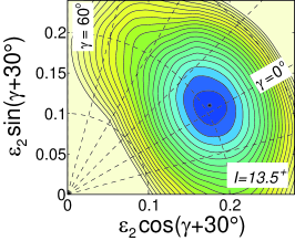
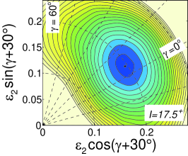
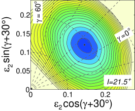
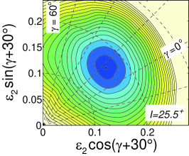
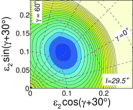
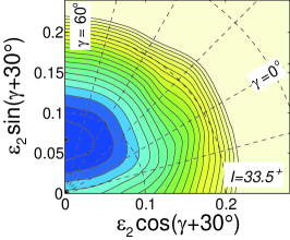
Figure 16: (Color online) Evolution of the potential energy surfaces (PES) for the [20,2] configuration in ¹⁰⁷In. The six PES figures are given in steps of $4\hbar$ from the near-prolate state at $I=13.5^{+}$ up to the terminating state at $I=33.5^{+}$. The energy difference between two neighboring equipotential lines is 0.2 MeV and the last equipotential line corresponds to 4.0 MeV excitation with respect to the minimum.

V Summary

In summary, a rotational band structure with ten E2 cascade transitions has been observed in ¹⁰⁷In. The J⁽¹⁾ and J⁽²⁾ moments of the band exhibit a gradual decrease with increasing rotational frequency, a typical characteristic of the smoothly terminating bands in this mass region. The experimental results were compared with Total Routhian Surface (TRS) and Cranked Nilsson-Strutinsky (CNS) calculations. In the former case, pairing was taken into account and in the latter, it was neglected. In both calculations, the configuration with positive parity and negative signature $(+,-1/2)$ was energetically most favored in the spin range $I=20-31\hbar$. According to the CNS calculations, the observed band has a [20,2] structure: under this configuration assignment it is one transition short of termination. However, the TRS calculations give some preference for a negative parity assignment instead, corresponding to an approximate [21,2] configuration at high spin using the CNS labels. Further experimental investigations of this nucleus will be useful to observe higher spin levels and definitely fix the spin of the observed band.

- (1) A. Gadea et al., Phys. Rev. C 55, R1 (1997).
- (2) I. Ragnarsson, V.P. Janzen, D.B. Fossan, N.C. Schmeing, and R. Wadsworth, Phys. Rev. Lett. 74, 3935 (1995).
- (3) V.P. Janzen et al., Phys. Rev. Lett., 72, 1160 (1994).
- (4) A. V. Afanasjev, D. B. Fossan, G. J. Lane and I. Ragnarsson, Phys. Rep. 322, 1 (1999).
- (5) A. O. Evans et al., Phys. Lett. B636, 25 (2006).
- (6) R. Wadsworth et al., Phys. Rev. C 53, 2763 (1996).
- (7) E. S. Paul et al., Phys. Rev. C76, 034323 (2007).
- (8) S.K. Tandel et al., Phys. Rev. C 58, 3738 (1998).
- (9) S. Sihotra et al., Eur. Phys. J. A 43, 45 (2010).
- (10) C.W. Beqausang et al., Nucl. Instrum. and Methods Phys. Res. A 313, 37 (1992).
- (11) M. Leino et al., Nucl. Instrum. and Methods Phys. Res. B 99, 653 (1995).
- (12) M. Leino et al., Nucl. Instrum. and Methods Phys. Res. B 126, 320 (1997).
- (13) R.D. Page et al., Nucl. Instrum. and Methods Phys. Res. B 204, 634 (2003).
- (14) I.H. Lazarus et al., IEEE Trans. Nucl. Sci. 48, 567 (2001).
- (15) P. Rahkila, Nucl. Instrum. and Methods Phys. Res. A 595, 637 (2008).
- (16) D.C. Radford, Nucl. Instrum. Methods Phys. Res. A361, 297 (1995).
- (17) W. Andrejtscheff et al., Z. Phys. A 328, 23 (1987).
- (18) P. Singh, R.G. Pillay, J.A. Sheikh, and H.G. Devare, Phys. Rev. C 45, 2161 (1992).
- (19) D. Jerrestam et al., Phys. Rev. C 52, 2448 (1995).
- (20) P.H. Regan et al., Nucl. Phys. A586, 351 (1995).
- (21) R. Wadsworth et al., Phys. Rev. Lett. 80, 1174 (1998).
- (22) H. Schnare et al., Phys. Rev. C 54, 1598 (1996).
- (23) E.S. Paul et al., Phys. Rev. C 61, 064320 (2000).
- (24) A. V. Afanasjev and I. Ragnarsson, Nucl. Phys. A591, 387 (1995).
- (25) R. Wadsworthet al., Nucl. Phys. A559, 461 (1993).
- (26) S. Cwiok et al., Comp. Phys. Commun. 46, 379 (1987).
- (27) W. Satula, R. Wyss, Phys. Scr. T 56, 159 (1995).
- (28) W. Satula, R. Wyss, P. Magierski, Nucl. Phys. A578, 45 (1994).
- (29) Y. Nogami, H.C. Pradhan, J. Law, Nucl. Phys. A201, 357 (1973).
- (30) J.-y. Zhang, N. Xu, D. B. Fossan, Y. Liang, R. Ma, and E. S. Paul, Phys. Rev. C 39, 714 (1989).
- (31) B. G. Carlsson, and I. Ragnarsson, Phys. Rev. C 74, 011302(R) (2006).