On Linear Operator Channels over Finite Fields

Abstract

Motivated by linear network coding, communication channels perform linear operation over finite fields, namely linear operator channels (LOCs), are studied in this paper. For such a channel, its output vector is a linear transform of its input vector, and the transformation matrix is randomly and independently generated. The transformation matrix is assumed to remain constant for every $T$ input vectors and to be unknown to both the transmitter and the receiver. There are NO constraints on the distribution of the transformation matrix and the field size.

Specifically, the optimality of subspace coding over LOCs is investigated. A lower bound on the maximum achievable rate of subspace coding is obtained and it is shown to be tight for some cases. The maximum achievable rate of constant-dimensional subspace coding is characterized and the loss of rate incurred by using constant-dimensional subspace coding is insignificant.

The maximum achievable rate of channel training is close to the lower bound on the maximum achievable rate of subspace coding. Two coding approaches based on channel training are proposed and their performances are evaluated. Our first approach makes use of rank-metric codes and its optimality depends on the existence of maximum rank distance codes. Our second approach applies linear coding and it can achieve the maximum achievable rate of channel training. Our code designs require only the knowledge of the expectation of the rank of the transformation matrix. The second scheme can also be realized ratelessly without a priori knowledge of the channel statistics.

I Introduction

Let $\mathbb{F}$ be a finite field with $q$ elements. A linear operator channel (LOC) with input $X\in\mathbb{F}^{T\times M}$ and output $Y\in\mathbb{F}^{T\times N}$ is given by

$$Y=XH,$$ (1)

where $H$ is called the transformation matrix.

Our motivation to study LOCs comes from linear network coding, a research topic that has drawn extensive interest in the past ten years. Linear network coding is a network transmission technique that can achieve the capacity of multicasting in communication networks [1, 2, 3, 4]. Different from routing, linear network coding allows network nodes to relay new packets generated by linear combinations. The point-to-point transmission of a network employing linear network coding is given by a LOC, where $H$ is the model of network transfer matrix and depends on the network topology [2, 3].

A recent research topic where LOCs have found applications is the deterministic model of wireless networks [5, 6]. This deterministic model provides a good approximation of certain wireless network behaviors and has shown its impact on the study of wireless networks. When employing linear operations in intermediate network nodes, the point-to-point transmission of the deterministic model of wireless networks is also given by a LOC [7, 8].

Even though some aspects of LOCs have been well studied in linear network coding, our understanding of LOCs is far from enough. In fact, the only case that LOCs are completely understood is that $H$ has a constant rank $M$. However, $H$ in general can have rank deficiency (i.e., $\operatorname{\text{rk}}(H)<M$) due to the change of network topology, link failure, packet loss, and so on. Even without these network related dynamics, $H$ has a random rank when random linear network coding is applied where new packets are generated by random linear combinations. Towards more sophisticated applications of linear network coding, a systematic study of LOCs becomes necessary. In this work, we study the information theoretic communication limits of LOCs with a general distribution of $H$ and discuss coding for LOCs.

I-A Some Related Works

We review some works of linear network coding that related to our discussions.

When both the transmitter and the receiver know the instances of $H$, the transmission through a LOC is called the coherent transmission. For a network with fixed and known topology, linear network codes can be designed deterministically in polynomial time [4]. The transmission through such a network is usually assumed to be coherent. For the coherent transmission, the rank of $H$ determines the capability of information transmission and it is bounded by the maximum flow form the transmitter to the receiver [2, 3, 5, 6].

In communication networks where the network topology is dynamic and/or unknown, e.g., wireless communication networks, deterministic design of network coding is difficult to realize. Random linear network coding is an efficient approach to apply network coding in such communication networks [9, 10, 11, 12, 13]. The transformation matrix of a communication network employing random linear network coding, called a random linear coding network (RLCN), is a random matrix and its instances are assumed to be unknown in both the transmitter and the receiver. Such a kind of transmission is referred to as the noncoherent transmission. The existing works on the noncoherent transmission of RLCN considers several special distributions of $H$.

In various models and applications of random linear network coding [9, 14, 15, 16, 17], $H$ is assumed to be an invertible square matrix. This assumption is based on the fact that when $H$ is a square matrix, i.e., $M=N$, it is full rank with high probability if i) $M$ is less than or equal to the maximum flow from the transmitter to the receiver, and ii) the field size for network coding is sufficiently large comparing with the number of network nodes [9, 18]. However, random linear network coding with small finite fields is attractive for low computing complexity. For example, wireless sensor networks is characterized by large network size and limited computing capability of network nodes. Using large finite field operations in sensors may not be a good choice. Moreover, the maximum flow varies due to the dynamic of wireless networks. For these reasons, full rank transformation matrices cannot be assumed in many applications.

Kötter and Kschischang [19] introduced a model of random linear network coding, called Kötter-Kschischang operator channel (or KK operator channel), that takes vector spaces as input and output, and commits fixed dimension erasures and additive errors. Their model considers a special kind of rank-deficiency of $H$ that gives fixed dimension erasures, defined as the difference of the dimension of the output and input vector spaces. They introduced subspace coding for random linear network coding that can be used to correct erasures, defined as the rank difference between the output and input matrices, as well as additive errors [19]. Silva et al. [20] constructed (unit-block) subspace codes using rank-metric codes [21], called unit-block lifted rank-metric codes here, which are nearly optimal in terms of achieving a Singleton type bound of (unit-block) subspace codes [19]. The coding scheme proposed by Ho et al.[9] for random linear network coding is a special case of unit-length lifted rank-metric codes for the transmission without erasures and errors.

Jafari et al.[22, 23] studied $H$ containing uniformly i.i.d. components—such a matrix is called a purely random matrix. However, there is no rigorous justification of why purely random matrices can reflect the properties of general random linear network coding. Moreover, the problem-specific techniques used to analyze purely matrices are difficult to be extended to the general cases.

I-B Summary of Our Work

In this paper, we study LOCs without any constraints on the distribution of $H$. The purely random transformation matrix and the invertible transformation matrix are special cases in our problem. We allow the transformation matrix has arbitrary rank and contains correlated components. We do not assume large finite fields to guarantee that the rank of $H$ is full rank with high probability. We mainly consider the noncoherent transmission of LOCs by assuming the instances of $H$ is unknown in both the transmitter and the receiver.

Our results can be applied to (random) linear network coding in both wireless and wireline networks without constraints on the network topology and the field size, as long as the input and output of the network can be modelled by a LOC. For example, link failures and packets losses, which do not change the linear relation between the input and output, can be taken into consideration. But the network transformation can also suffers from random errors and malicious modifications, for which we have to model the network transformation as

$$Y=XH+Z,$$

and there is no equivalent way to model it as a LOC. We do not consider nonzero $Z$ as discussed in [19, 14, 15].

Our results are summarized as follows.

We generalize the concept of subspace coding in [19] to multiple usages of a LOC and study its achievable rates. Let $\bar{C}$ be the capacity of a LOC and let $\bar{C}_{\text{SS}}$ be the maximum achievable rate of subspace coding for a LOC. We obtain that $(1-M/T)\operatorname{E}[\operatorname{\text{rk}}(H)]+\epsilon(T,q)\leq\bar{C}_{\text{SS}}\leq\bar{C}\leq\operatorname{E}[\operatorname{\text{rk}}(H)]$, where $\operatorname{E}[\operatorname{\text{rk}}(H)]$ is the expectation of the rank of $H$ and $0<\epsilon(T,q)<1.8/(T\log_{2}q)$. Moreover, we show that $\bar{C}_{\text{SS}}=\bar{C}$ for uniform LOCs, a class of LOCs that includes the purely random transformation matrix and the invertible transformation matrix studied in [15, 22, 23].

An unknown transformation matrix is regular if its rank can take any value from zero to $M$. A LOC is regular if its transformation matrix is regular. For regular LOCs with sufficiently large $T$, we prove that the lower bound on $\bar{C}_{\text{SS}}$ is tight, and $\bar{C}_{\text{SS}}$ is achieved by the $M$-dimensional subspace coding. For example, a purely random $H$ with $M\leq N$ is uniform and regular. Thus $M$-dimensional subspace coding achieves its capacity when $T$ is sufficiently large.

Moreover, $\bar{C}_{\text{SS}}$ can be well approximated by subspace codes using subspaces with the same dimension, called constant-dimensional subspace codes. Let $\bar{C}_{\text{C-SS}}$ be the maximum achievable rate of constant-dimensional subspace coding. We show that $\bar{C}_{\text{SS}}-\bar{C}_{\text{C-SS}}<(\log_{2}\min\{M,N\})/(T\log_{2}q)$, which is much smaller than $\bar{C}_{\text{SS}}$ for practical channel parameters. For general LOCs, we find the optimal dimension $r^{*}$ such that there exists an $r^{*}$-dimensional subspace code achieving $\bar{C}_{\text{C-SS}}$. Taking the LOCs with an invertible $H$ as an example, $M$ is the optimal dimension when $T\geq 2M+1$.

Channel training is a coding scheme for LOCs that uses parts of its input matrix to recover the instance of $H$. The maximum achievable rate of using channel training $\bar{C}_{\text{CT}}$ is $(1-M/T)\operatorname{E}[\operatorname{\text{rk}}(H)]$, which is very close to the lower bound of $\bar{C}_{\text{SS}}$. We further proposed extended channel training codes to reducing the overhead of channel training codes. We give upper and lower bounds on the maximum achievable rate of extended channel training codes and show the gap between bounds is small.

The coding scheme proposed by Ho et al.[9] and the unit-block lifted rank-metric codes proposed by Silva et al.[20] fall in the class of channel training. We show that unit-block lifted rank-metric codes can achieve $\bar{C}_{\text{CT}}$ only when $H$ has a constant rank. If $H$ have an arbitrary rank, the maximum achievable rate of unit-block lifted rank-metric codes is demonstrated to be far from $\bar{C}_{\text{CT}}$ for certain rank distribution of $H$.

To achieve $\bar{C}_{\text{CT}}$, we consider two coding schemes. In the first scheme, we extend the method of Silva et al. [20] to construct codes for LOCs by multiple uses of the channel. The constructed code is called lifted rank-metric code. The optimality of lifted rank-metric codes, in the sense of achieving $\bar{C}_{\text{CT}}$, depends on the existence of the maximum-rank-distance (MRD) codes in classical algebraic coding theory, which was first studied in [21]. Specifically, we show that if $T\gg M$, lifted rank-metric codes can approximately approach $\bar{C}_{\text{CT}}$. Otherwise, since the existence of MRD codes is unclear, it is uncertain if lifted rank-metric codes can achieve $\bar{C}_{\text{CT}}$. Exsiting decoding algorithms of rank-metric codes can be applied to lifted rank-metric codes. The decoding complexity is given by $\mathcal{O}(n^{2})$ field operations in $\mathbb{F}$, where $n$ is the block length of the codes.

We further propose a class of codes called lifted linear matrix codes, which can achieve $\bar{C}_{\text{CT}}$ for all $T\geq M$. We show that with probability more than half, a randomly choosen generator matrix gives good performance. We obain the error exponent of decoding lifted linear matrix codes. The decoding of a lifted linear matrix code has complexity given by $\mathcal{O}(n^{3})$ field operations when applying Gaussian elimination. Lifted linear matrix codes can be realized ratelessly if the channel has a neglectable rate of feedback.

Both lifted rank-metric codes and lifted linear matrix codes are universal in the sense that i) only the knowledge of $\operatorname{E}[\operatorname{\text{rk}}(H)]$ is required to design codes and ii) a code has similar performance for all LOCs with the same $\operatorname{E}[\operatorname{\text{rk}}(H)]$. Furthermore, rateless lifted linear matrix codes do not require any priori knowledge of channel statistics.

I-C Organization

This paper also provides a general framework to study LOCs. Some notations and mathematical results that are used in our discussion, including some counting problems related to projective spaces, are introduced in §II. Self-contained proofs of these counting problems are given in Appendix A. In §III, linear operator channels are formally defined, and coherent and noncoherent transmission of LOCs are discussed. In §IV we give the maximum achievable rate of a noncoherent transmission scheme: channel training and study the bounds on the maximum achievable rate of extended channel training. In §V, we reveal an intrinsic symmetric property of LOCs that holds for any distribution of the transformation matrix. These symmetric properties can help to determine the capacity-achieving input distributions of LOCs. In §VI and §VII we study subspace coding. From §VIII to §X, two coding approaches for LOCs are introduced. The last section contains the concluding remarks.

II Preliminaries

Let $\mathbb{F}$ be the finite field with $q$ elements, $\mathbb{F}^{t}$ be the $t$-dimensional vector space over $\mathbb{F}$, and $\mathbb{F}^{t\times m}$ be the set of all $t\times m$ matrices over $\mathbb{F}$. For a matrix $\mathbf{X}$, let $\operatorname{\text{rk}}(\mathbf{X})$ be its rank, let $\mathbf{X}^{\top}$ be its transpose, and let $\langle\mathbf{X}\rangle$ be its column space, the subspace spanned by the column vectors of $\mathbf{X}$. Similarly, the row space of $\mathbf{X}$ is denoted by $\langle\mathbf{X}^{\top}\rangle$. If $V$ is a subspace of $U$, we write $V\leq U$.

The projective space $\operatorname{Pj}(\mathbb{F}^{t})$ is the collection of all subspaces of $\mathbb{F}^{t}$. Let $\operatorname{Pj}(m,\mathbb{F}^{t})$ be the subset of $\operatorname{Pj}(\mathbb{F}^{t})$ that contains all the subspaces with dimension less than or equal to $m$. This paper involves some counting problems in projective space, which are discussed in Appendix A. Let $\operatorname{Fr}(\mathbb{F}^{m\times r})$ be the set of full rank matrices in $\mathbb{F}^{m\times r}$. Define

$$\chi^{m}_{r}=\left\{\begin{array}[]{ll}(q^{m}-1)(q^{m}-q)\cdots(q^{m}-q^{r-1})&r>0\\ 1&r=0\end{array}\right.$$ (2)

for $r\leq m$. By Lemma 10, $|\operatorname{Fr}(\mathbb{F}^{m\times r})|=\chi^{m}_{r}$. Define

$$\zeta^{m}_{r}=\chi^{m}_{r}q^{-mr}.$$ (3)

Since the number of $m\times r$ matrices is $q^{mr}$, $\zeta^{m}_{r}$ can be regarded as the probability that a randomly chosen $m\times r$ matrix is full rank (ref. Lemma 11). The Grassmannian $\operatorname{Gr}(r,\mathbb{F}^{t})$ is the set of all $r$-dimensional subspaces of $\mathbb{F}^{t}$. Thus $\operatorname{Pj}(m,\mathbb{F}^{t})=\bigcup_{r\leq m}\operatorname{Gr}(r,\mathbb{F}^{t})$. The Gaussian binomials are defined as

$$\begin{pmatrix}m\\ r\end{pmatrix}_{q}=\frac{\chi^{m}_{r}}{\chi^{r}_{r}}.$$

By Lemma 12, $\left({}^{t}_{r}\right)_{q}=|\operatorname{Gr}(r,\mathbb{F}^{t})|$. Let

$$\chi^{m,n}_{r}=\frac{\chi^{m}_{r}\chi^{n}_{r}}{\chi^{r}_{r}},$$ (4)

which is the number of $m\times n$ matrices with rank $r$ (see Lemma 13).

For a discrete random variable (RV) $X$, we use $p_{X}$ to denote its probability mass function (PMF). Let $X$ and $Y$ be RVs over discrete alphabets $\mathcal{X}$ and $\mathcal{Y}$, respectively. We write a transition probability (matrix) from $\mathcal{X}$ to $\mathcal{Y}$ as $P_{Y|X}(\mathbf{X}|\mathbf{Y})$, $\mathbf{X}\in\mathcal{X}$ and $\mathbf{Y}\in\mathcal{Y}$. When the context is clear, we may omit the subscript of $p_{X}$ and $P_{Y|X}$ to simplify the notations.

III Linear Operator Channels

III-A Formulations

We first introduce a vector formulation of LOCs which reveals more details than the one given in (1). Let $T$, $M$ and $N$ be nonnegative integers. A linear operator channel takes an $M$-dimensional vector as input and an $N$-dimensional vector as output. The $i$th input $x_{i}\in\mathbb{F}^{1\times M}$ and the $i$th output $y_{i}\in\mathbb{F}^{1\times N}$ are related by

$$y_{i}=x_{i}H_{i},$$

where $H_{i}$ is a random matrix over $\mathbb{F}^{M\times N}$. We consider that $H_{i}$ keeps constant for $T$ consecutive input vectors, i.e.,

$$H_{nT+1}=H_{nT+2}=\cdots=H_{nT+T},\quad n=0,1,2,\cdots;$$

and $H_{nT+1}$, $n=0,1,\cdots$, are independent and follow the same generic distribution of random variable $H$. By considering $T$ consecutive inputs/outputs as a matrix, we have the matrix formulation given in (1). Here, $T$ is called the inaction period; $M\times N$ is called the dimension of the LOC. A LOC with transformation matrix $H$ and inaction period $T$ is denoted by $\text{LOC}(H,T)$. Unless otherwise specified, we use the capital letters $M$ and $N$ for the dimension of $\text{LOC}(H,T)$. We will use the matrix formulation of the LOCs in this paper exclusively. When we talk about one use of $\text{LOC}(H,T)$, we mean the channel transmits one $T\times M$ matrix.

A communication network employing linear network coding can be modeled by a LOC. For example, when applying linear network coding in relay nodes, the transformation matrix of the network in Fig. 1 is

$$H=\begin{bmatrix}\alpha_{1}&\alpha_{2}\beta_{1}\\ 0&\beta_{2}\end{bmatrix},$$ (5)

in which $\alpha_{1},\alpha_{2},\beta_{1}$ and $\beta_{2}$ are linear combination coefficients taking value in $\mathbb{F}$. These coefficients can be fixed or random depending on the linear network coding approach. For a given network topology, the general formulation of the transformation matrix of linear network coding can be found in [3].

For wireless networks without a centralized control, the transmission of network nodes is spontaneous and the network topology is dynamic. When employing random linear network coding, the inputs and the outputs of a wireless network still have linear relations [16], but the formulation of the transformation matrix is difficult to obtain. The instances of the transformation matrix of random network coding is usually assumed to be unknown in both the transmitter and the receiver. We will mainly discuss this kind of transmission of LOCs (see §III-C).

The transmission of random linear network coding is packetized. The source node organizes its data into $M$ packages, called a batch, and each of which contains $T$ symbols from $\mathbb{F}$. Network nodes perform linear network coding among the symbols in the same position of the packages in one batch, and the coding for all the positions are the same. This packetized transmission matches our assumption that the transformation matrix keeps constant for $T$ consecutive input vectors. For this reason, the inaction period is also called the packet length. The sink node try to collect $N$ (usually, $N\geq M$) packages in this batch to decode the original packages. This gives a physical meaning of the dimension of LOCs.

Figure 1: A directed network with the source node $s$ and the sink node $t$. Each edge in the network is a communication link that can transmit a symbol from $\mathbb{F}$ without error. Node $a$ and $b$ are rely nodes that apply linear network coding. The transmitted symbols through links are labeled.

III-B Coherent Transmission of LOCs

We call the instances of the transformation matrix the channel information (CI). The transmission with known CI at both the transmitter and the receiver is called coherent transmission. When the instance of $H$ is $\mathbf{H}$, the maximum achievable rate of coherent transmission is $\max_{p_{X}}I(X;Y|H=\mathbf{H})$. Thus, the maximum achievable rate of coherent transmission (also called the coherent capacity) is

$$C_{\text{co}}(H,T) =\sum_{\mathbf{H}}p_{H}(\mathbf{H})\max_{p_{X}}I(X;Y|H=\mathbf{H}).$$

Unless otherwise specified, we use a base-$2$ logarithm in this paper so that $C_{\text{co}}(H,T)$ has a bit unit.

Similar to coherent transmission, we can consider the transmission with CI only available at the receiver. We also assume that $X$ and $H$ are independent—this assumption is consistent with the transmitter does not know the instances of $H$. The maximum achievable rate of such transmission is

$$C_{\text{R-CI}}(H,T)=\max_{p_{X}}I(X;YH).$$

A random matrix is purely random if it has uniformly independent components.

Proposition 1

$C_{\text{R-CI}}(H,T)=C_{\text{co}}(H,T)={T\log_{2}q}\operatorname{E}[\operatorname{\text{rk}}(H)]$ and both capacities are achieved by the purely random input distribution.

Proof:

We first consider the coherent transmission. We know

$$I(X;Y|H=\mathbf{H}) =H(Y|H=\mathbf{H})-H(Y|X,H=\mathbf{H})$$

$$=H(Y|H=\mathbf{H}).$$

Let $x_{i}$ and $y_{i}$ be the $i$th rows of $X$ and $Y$, respectively. Since $y_{i}=x_{i}\mathbf{H}$, i.e., $y_{i}$ is a vector in the subspace spanned by the row vectors of $\mathbf{H}$,

$$H(y_{i}|H=\mathbf{H})\leq\log_{2}q^{\operatorname{\text{rk}}(\mathbf{H})}=\operatorname{\text{rk}}(\mathbf{H})\log_{2}q,$$

in which the equality is achieved when $x_{i}$ contains uniformly independent components. Hence,

$$H(Y|H=\mathbf{H}) \leq\sum_{i=1}^{T}H(y_{i}|H=\mathbf{H})$$

$$\leq\operatorname{\text{rk}}(\mathbf{H})T\log_{2}q,$$

where the first equality is achieved when $x_{i}$, $i=1,\cdots,T$, are independent. Therefore,

$$C_{\text{co}}(H,T) =\sum_{\mathbf{H}}p_{H}(\mathbf{H})\max_{p_{X}}I(X;Y|H=\mathbf{H})$$

$$=\sum_{\mathbf{H}}p_{H}(\mathbf{H})\operatorname{\text{rk}}(\mathbf{H})T\log_{2}q$$

$$=\operatorname{E}[\operatorname{\text{rk}}(H)]T\log_{2}q.$$

Now we consider the transmission with CI only available at the receiver. We know

$$I(X;YH) =I(X;Y|H)+I(X;H)$$

$$=I(X;Y|H)$$

$$=H(Y|H)-H(Y|XH)$$

$$=H(Y|H),$$

in which $I(X;H)=0$ since $X$ and $H$ are independent. Similar to the coherent case,

$$H(Y|H) =\sum_{\mathbf{H}}p_{H}(\mathbf{H})H(Y|H=\mathbf{H})$$

$$\leq\sum_{i=1}^{T}\sum_{\mathbf{H}}p_{H}(\mathbf{H})H(y_{i}|H=\mathbf{H})$$

$$\leq\sum_{i=1}^{T}\sum_{\mathbf{H}}p_{H}(\mathbf{H})\operatorname{\text{rk}}(\mathbf{H})\log_{2}q$$

$$=\operatorname{E}[\operatorname{\text{rk}}(H)]T\log_{2}q,$$

where the equality is achieved by $X$ with uniformly independent components. ∎

Remark: Note that we do not assume $X$ and $H$ are independent for coherent transmission. In fact for coherent transmission, the transmitter can use its knowledge of $\mathbf{H}$ in encoding. Without lose of generality, we assume that the first $\operatorname{\text{rk}}(\mathbf{H})$ rows of $\mathbf{H}$ are linearly independent. So the transmitter can encode its information in an $M$-dimensional vector which contains only nonzero values in its first $\operatorname{\text{rk}}(\mathbf{H})$ components. The receiver can decode these nonzero values by solving a linear system of equations. Such scheme has transmission rate $\operatorname{\text{rk}}(\mathbf{H})T\log_{2}q$, which achieves the coherent capacity. The coding that achieves $\operatorname{E}[\operatorname{\text{rk}}(H)]T\log_{2}q$ with CI only available at the receiver, discussed in §VIII, is more involved.

III-C Noncoherent Transmission of LOCs

The transmission without the knowledge of CI in both the transmitter and the receiver is called noncoherent transmission. Same to the case with CI only available at the receiver, we assume that $H$ and $X$ are independent for noncoherent transmission. Under this assumption,

$$p_{XY}(\mathbf{X},\mathbf{Y}) =\Pr\{X=\mathbf{X},Y=\mathbf{Y}\}$$

$$=\Pr\{X=\mathbf{X},\mathbf{X}H=\mathbf{Y}\}$$

$$=\Pr\{X=\mathbf{X}\}\Pr\{\mathbf{X}H=\mathbf{Y}\}.$$

Thus, the transition probability $P_{Y|X}(\mathbf{Y}|\mathbf{X})$ of noncoherent transmission is given by

$$P_{Y|X}(\mathbf{Y}|\mathbf{X})=\Pr\{\mathbf{X}H=\mathbf{Y}\}.$$ (6)

Unless otherwise specified, we consider noncoherent transmission of LOCs in the rest of this paper. For noncoherent transmission, a LOC is a discrete memoryless channel (DMC). The (noncoherent) capacity of $\text{LOC}(H,T)$ is

$$C(H,T)=\max_{p_{X}}I(X;Y).$$

We also consider the normalized channel capacity

$$\bar{C}(H,T)=\frac{C(H,T)}{T\log_{2}q}.$$

When we talk about the normalization of a coding rate, we mean to normalize by $T\log_{2}q$.

Achieving the capacity generally involves multiple usages of the channel. A block code for $\text{LOC}(H,T)$ is a subset of $(\mathbb{F}^{T\times M})^{n}$, the $n$th Cartesian power of $\mathbb{F}^{T\times M}$. Here $n$ is the length of the block code. Since the components of codewords are matrices, such a code is called a matrix code. The channel capacity of a LOC can be approached using a sequence of matrix codes with $n\rightarrow\infty$.

In the following subsection, we give the channel capacity and the capacity achieving inputs of three LOCs. These examples show that finding the channel capacity is problem-specific. In general, it is not easy to accurately characterize the (noncoherent) capacity of a LOC. Since an input distribution contains $q^{TM}$ probability masses, a general method to maximize a mutual information, e.g., the Blahut-Arimoto algorithm, has time complexity $\mathcal{O}(q^{TM})$. Moreover, the distribution of the transformation matrix is difficult to obtain in applications like random linear network coding. Therefore, our goal is to find an efficient method to approach the capacity of LOCs with limited channel statistics.

III-D Examples of Linear Operator Channels

III-D1 $Z$-Channel

A $Z$-channel with crossover probability $p$ is a binary-input-binary-output channel that flips the input bit $1$ with probability $p$, but maps input bit $0$ to $0$ with probability $1$. A $Z$-channel is a LOC over binary field given by

$$y=xh,$$

where $\Pr\{h=0\}=p$. We know the capacity of a $Z$-channel is $C(h,1)=\log_{2}\left(1+(1-p)p^{p/(1-p)}\right)$, which is achieved by

$$p_{x}(0)=\frac{1-p^{1/(1-p)}}{1+(1-p)p^{p/(1-p)}}.$$

III-D2 Full Rank Transformation Matrix

Let $H_{\text{full}}$ be the random matrix uniformly distributed over $\operatorname{Fr}(\mathbb{F}^{M\times N})$, $M\leq N$. For $\text{LOC}(H_{\text{full}},T)$,

$$P_{Y|X}(\mathbf{Y}|\mathbf{X})=\left\{\begin{array}[]{ll}\frac{1}{\chi^{N}_{\operatorname{\text{rk}}(\mathbf{X})}}&\langle\mathbf{Y}\rangle=\langle\mathbf{X}\rangle\\ 0&o.w..\end{array}\right.$$

This kind of transformation matrix with $M=N$ has been studied in [15]. Let $M^{*}=\min\{M,T\}$. We know

$$C(H_{\text{full}},T)=\log_{2}\sum_{r\leq M^{*}}\left({}^{T}_{r}\right)_{q},$$

where $\sum_{r\leq M^{*}}\left({}^{T}_{r}\right)_{q}=|\operatorname{Pj}(M^{*},\mathbb{F}^{T})|$. Any input $p_{X}$ satisfying

$$p_{\langle X\rangle}(U)=\frac{1}{|\operatorname{Pj}(M^{*},\mathbb{F}^{T})|},\quad\forall U\in\operatorname{Pj}(M^{*},\mathbb{F}^{T}),$$

is capacity achieving. In other words, this capacity is achieved by using each subspace in $\operatorname{Pj}(M^{*},\mathbb{F}^{T})$ uniformly.

III-D3 Purely Random Transformation Matrix

Recall that a random matrix is called purely random if it contains uniformly independent components. Consider $\text{LOC}(H_{\text{pure}},T)$ with purely random $H_{\text{pure}}$ and dimension $M\times N$. We have

$$P_{Y|X}(\mathbf{Y}|\mathbf{X})=\left\{\begin{array}[]{ll}q^{-N\operatorname{\text{rk}}(\mathbf{X})}&\langle\mathbf{Y}\rangle\subseteq\langle\mathbf{X}\rangle\\ 0&o.w..\end{array}\right.$$

Such channels were studied in [22, 23], where the capacity formulas, involving big-O notations, are obtained for different cases. We will give an exact formula for sufficiently large $T$,

$$C(H_{\text{pure}},T)=\operatorname{E}\left[\log_{2}\frac{\chi^{T}_{\operatorname{\text{rk}}(H)}}{\chi^{M}_{\operatorname{\text{rk}}(H)}}\right].$$

This capacity is achieved by an input $p_{X}$ with

$$p_{X}(\mathbf{X})=\left\{\begin{array}[]{ll}1/\chi^{T}_{M}&\operatorname{\text{rk}}(\mathbf{X})=M\\ 0&o.w..\end{array}\right.$$

In other words, this capacity is achieved by using all the full rank $T\times M$ matrices with equal probability.

IV Channel Training

In noncoherent transmission, the CI is not available in either the transmitter or the receiver. But we can deliver the CI to the receiver using a simple channel training technique. When $T\geq M$, we can transmit an identity $M\times M$ matrix as a submatrix of $X$ to recover $H$ at the receiver. For example, if

$$X=\begin{bmatrix}\mathbf{I}\\ X^{\prime}\end{bmatrix},$$

then

$$Y=XH=\begin{bmatrix}H\\ X^{\prime}H\end{bmatrix}.$$

The first $M$ rows of $Y$ gives the instance of $H$. Thus the last $T-M$ rows of $Y$ can be decoded with the CI. Let $C_{\text{CT}}$ be the maximum achievable rate of such a scheme, and $\bar{C}_{\text{CT}}$ be its normalization.

Proposition 2

For $\text{LOC}(H,T)$ with dimension $M\times N$ and $T\geq M$, $\bar{C}_{\text{CT}}=(1-M/T)\operatorname{E}[\operatorname{\text{rk}}(H)]$.

Proof:

Let $\tilde{X}$ be a random matrix over $\mathbb{F}^{(T-M)\times M}$ and let $\tilde{Y}=\tilde{X}H$. If the input of $\text{LOC}(H,T)$ is $X=\begin{bmatrix}\mathbf{I}\\ \tilde{X}\end{bmatrix}$, the output is $Y=\begin{bmatrix}\mathbf{I}\\ \tilde{X}\end{bmatrix}H=\begin{bmatrix}H\\ \tilde{Y}\end{bmatrix}$. Thus,

$$\bar{C}_{\text{CT}} =\max_{p_{X}}I(X;Y)/(T\log_{2}q)$$

$$=\max_{p_{\tilde{X}}}I(\tilde{X};\tilde{Y}H)/(T\log_{2}q).$$

Since $\tilde{X}$ and $H$ are independent, we have

$$I(\tilde{X};\tilde{Y}H) =I(\tilde{X};\tilde{Y}|H)$$

$$=H(\tilde{Y}|H)$$

$$\leq\operatorname{E}[\operatorname{\text{rk}}(H)](T-M)\log_{2}q,$$

where the equality is achieved by $\tilde{X}$ with uniformly independent components. ∎

Remark: In this formula of $\bar{C}_{\text{CT}}(H,T)$, $M/T$ is just the ratio of the overhead used in channel training.

Corollary 1

$(1-M/T)\operatorname{E}[\operatorname{\text{rk}}(H)]\leq\bar{C}(H,T)\leq\operatorname{E}[\operatorname{\text{rk}}(H)]$.

Proof:

It follows from ${C}_{\text{CT}}(H,T)\leq{C}(H,T)\leq{C}_{\text{R-CI}}(H,T)$. ∎

The upper bound and the lower bound is asymptotically tight when $T$ is large. We will further improve the lower bound by showing that the inequality is strict.

Now we consider how to improve $\bar{C}_{\text{CT}}(H,T)$ by reducing the overhead ratio $M/T$. The method is to apply channel training to the new channel $\text{LOC}(GH,T)$ for a random matrix $G$ with dimension $r\times M$. See that $\bar{C}_{\text{CT}}(GH,T)=(1-r/T)\operatorname{E}[\operatorname{\text{rk}}(GH)]\leq(1-r/T)\operatorname{E}[\operatorname{\text{rk}}(H)]$. Thus, to achieve higher rate than $(1-M/T)\operatorname{E}[\operatorname{\text{rk}}(H)]$, we only need to consider $r<M$. We call this method extended channel training. The maximum achievable rate of extended channel training is

$$\bar{C}_{\text{ECT}}(H,T)=\max_{r\leq M}\sup_{p_{G}:\text{The dimension of }G\text{ is }r\times M}(1-r/T)\operatorname{E}[\operatorname{\text{rk}}(GH)].$$

Theorem 1

For $\text{LOC}(H,T)$ with dimension $M\times N$, we have

$$\bar{C}_{\text{ECT}}(H,T)\geq\max\left\{\max_{r<M}(1-r/T)\left(\sum_{k=0}^{r-1}p_{\operatorname{\text{rk}}(H)}(k)k\zeta^{r}_{k}+r\sum_{k=r}^{M}p_{\operatorname{\text{rk}}(H)}(k)\zeta^{k}_{r}\right),\bar{C}_{\text{CT}}(H,T)\right\},$$

and

$$\bar{C}_{\text{ECT}}(H,T)\leq\max_{r\leq M}(1-r/T)\left(\sum_{k=0}^{r-1}p_{\operatorname{\text{rk}}(H)}(k)k+r\sum_{k=r}^{M}p_{\operatorname{\text{rk}}(H)}(k)\right).$$

Proof:

We have that

$$\operatorname{E}[\operatorname{\text{rk}}(GH)] =\sum_{s=0}^{r}s\Pr\{\operatorname{\text{rk}}(GH)=s\}$$

$$=\sum_{s=0}^{r}s\sum_{k=s}^{M}\Pr\{\operatorname{\text{rk}}(GH)=s|\operatorname{\text{rk}}(H)=k\}p_{\operatorname{\text{rk}}(H)}(k)$$

$$=\sum_{k=0}^{M}p_{\operatorname{\text{rk}}(H)}(k)\sum_{s\leq\min\{k,r\}}s\Pr\{\operatorname{\text{rk}}(GH)=s|\operatorname{\text{rk}}(H)=k\}.$$

To prove the first inequality, we consider $G$ is purely random. By Lemma 13, $\Pr\{\operatorname{\text{rk}}(GH)=s|\operatorname{\text{rk}}(H)=k\}=\frac{\zeta^{k}_{s}\zeta^{r}_{s}}{\zeta^{s}_{s}q^{(k-s)(r-s)}}$. Then,

$$\operatorname{E}[\operatorname{\text{rk}}(GH)] =\sum_{k=0}^{M}p_{\operatorname{\text{rk}}(H)}(k)\sum_{s\leq\min\{k,r\}}s\frac{\zeta^{k}_{s}\zeta^{r}_{s}}{\zeta^{s}_{s}q^{(k-s)(r-s)}}$$

$$=\sum_{k=0}^{r-1}p_{\operatorname{\text{rk}}(H)}(k)\sum_{s\leq k}s\frac{\zeta^{k}_{s}\zeta^{r}_{s}}{\zeta^{s}_{s}q^{(k-s)(r-s)}}+\sum_{k=r}^{M}p_{\operatorname{\text{rk}}(H)}(k)\sum_{s\leq r}s\frac{\zeta^{k}_{s}\zeta^{r}_{s}}{\zeta^{s}_{s}q^{(k-s)(r-s)}}$$

$$>\sum_{k=0}^{r-1}p_{\operatorname{\text{rk}}(H)}(k)k\zeta^{r}_{k}+\sum_{k=r}^{M}p_{\operatorname{\text{rk}}(H)}(k)r\zeta^{k}_{r}.$$

Therefore

$$\bar{C}_{\text{ECT}}(H,T) =\max\left\{\max_{r<M}\sup_{p_{G}:\text{The dimension of }G\text{ is }r\times M}(1-r/T)\operatorname{E}[\operatorname{\text{rk}}(GH)],(1-M/T)\operatorname{E}[\operatorname{\text{rk}}(H)]\right\}$$

$$=\max\left\{\max_{r<M}(1-r/T)\operatorname{E}[\operatorname{\text{rk}}(GH)]|_{G\text{ is purely random}},(1-M/T)\operatorname{E}[\operatorname{\text{rk}}(GH)]\right\}$$

$$\geq\max\left\{\max_{r<M}(1-r/T)\left(\sum_{k=0}^{r-1}p_{\operatorname{\text{rk}}(H)}(k)k\zeta^{r}_{k}+\sum_{k=r}^{M}p_{\operatorname{\text{rk}}(H)}(k)r\zeta^{k}_{r}\right),(1-M/T)\operatorname{E}[\operatorname{\text{rk}}(GH)]\right\}.$$

To prove the second inequality, we see that

$$\operatorname{E}[\operatorname{\text{rk}}(GH)] =\sum_{s=0}^{r}s\Pr\{\operatorname{\text{rk}}(GH)=s\}$$

$$=\sum_{s=0}^{r}s\sum_{k=s}^{M}\Pr\{\operatorname{\text{rk}}(GH)=s|\operatorname{\text{rk}}(G)=k\}p_{\operatorname{\text{rk}}(G)}(k)$$

$$=\sum_{k=0}^{r}p_{\operatorname{\text{rk}}(G)}(k)\sum_{s\leq k}s\Pr\{\operatorname{\text{rk}}(GH)=s|\operatorname{\text{rk}}(G)=k\}.$$

By

$$\sum_{s\leq k}s\Pr\{\operatorname{\text{rk}}(GH)=s|\operatorname{\text{rk}}(G)=k\} =\sum_{r\leq k}\sum_{s\geq r}\Pr\{\operatorname{\text{rk}}(GH)=s|\operatorname{\text{rk}}(G)=k\}$$

$$=\sum_{r\leq k}\Pr\{\operatorname{\text{rk}}(GH)\geq r|\operatorname{\text{rk}}(G)=k\}$$

$$\leq\sum_{r\leq k}\Pr\{\operatorname{\text{rk}}(H)\geq r\}$$

$$=\sum_{s<k}sp_{H}(s)+k\sum_{s\geq k}p_{H}(s),$$

we have

$$\operatorname{E}[\operatorname{\text{rk}}(GH)] =\sum_{k=0}^{r}p_{\operatorname{\text{rk}}(G)}(k)\left(\sum_{s<k}sp_{H}(s)+k\sum_{s\geq k}p_{H}(s)\right)$$

$$\leq\max_{k\leq r}\left(\sum_{s<k}sp_{H}(s)+k\sum_{s\geq k}p_{H}(s)\right).$$

The proof is completed. ∎

Corollary 2

Let $\bar{C}^{\text{upper}}_{\text{ECT}}(H,T)$ and $\bar{C}^{\text{lower}}_{\text{ECT}}(H,T)$ be the upper bound and the lower bound of $\bar{C}_{\text{ECT}}(H,T)$ in Theorem 1, respectively. When $T$ is sufficiently large,

$$\bar{C}^{\text{upper}}_{\text{ECT}}(H,T)-\bar{C}^{\text{lower}}_{\text{ECT}}(H,T)\leq\operatorname{E}[\operatorname{\text{rk}}(H)]\frac{M-r^{*}}{T},$$

where $r^{*}=\max\{r:p_{\operatorname{\text{rk}}(H)}(r)>0\}$. This means that if $p_{\operatorname{\text{rk}}(H)}(M)>0$, $\bar{C}^{\text{upper}}_{\text{ECT}}(H,T)=\bar{C}^{\text{lower}}_{\text{ECT}}(H,T)$ when $T$ is sufficiently large. Fixing the rank distribution of $H$, we have

$$\lim_{q\rightarrow\infty}\bar{C}^{\text{lower}}_{\text{ECT}}(H,T)=\bar{C}^{\text{upper}}_{\text{ECT}}(H,T).$$

Proof:

By the lower bound of $\bar{C}_{\text{ECT}}(H,T)$, we have $\bar{C}^{\text{lower}}_{\text{ECT}}(H,T)\geq(1-M/T)\operatorname{E}[\operatorname{\text{rk}}(H)]$. Let

$$a(r)=\sum_{s<r}sp_{H}(s)+r\sum_{s\geq r}p_{H}(s).$$

Since $a(r)=a(r^{*})$ for all $r>r^{*}$, we only need to consider $r\leq r^{*}$ to find the upper bound of $\bar{C}_{\text{ECT}}(H,T)$, i.e.,

$$\bar{C}^{\text{upper}}_{\text{ECT}}(H,T)=\max_{r\leq r^{*}}(1-r/T)a(r).$$

Fix $r<r^{*}$. We know that $a(r)<a(r^{*})$. Hence $(1-r/T)a(r)<(1-M/T)a(M)$ when $T\geq(r^{*}a(M)-ra(r))/(a(M-a(r))$. Therefore when $T\geq\max_{r<r^{*}}(r^{*}a(M)-ra(r))/(a(M)-a(r))$, $\bar{C}_{\text{ECT}}(H,T)=(1-r^{*}/T)\operatorname{E}[\operatorname{\text{rk}}(H)]$.

The second part of this corollary follows from $\zeta^{m}_{r}\rightarrow 1$ when $q\rightarrow\infty$. ∎

In Fig. 2, we illustrate the bounds of $\bar{C}_{\text{ECT}}(H,T)$ and $\bar{C}_{\text{CT}}(H,T)$ over binary field.

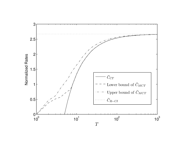
Figure 2: Here we fix an $H$ with $M=5$ and $p_{H}(M)=0$ over binary field. We plot the lower and upper bounds of $\bar{C}_{\text{ECT}}(H,T)$ and $\bar{C}_{\text{CT}}(H,T)$ for $T$ from $1$ to $1000$. Note that the bounds in this figure are only valid for integer T and hence, the curves are not necessarily smooth.

V Symmetric Property and Optimal Input Distributions

Here we introduce an intrinsic symmetric property of LOCs and show that this property is helpful to find an optimal input distribution of LOCs.

V-A Random Variables and Markov Chains Related to LOCs

We introduce several RVs related to LOCs, which are used extensively in this paper. Let $X$ be a RV over $\mathbb{F}^{t\times m}$. We denote by $\langle X\rangle$ as a RV over $\operatorname{Pj}(\mathbb{F}^{t})$ with

$$p_{\langle X\rangle}(U)=\Pr\{\langle X\rangle=U\}=\sum_{\mathbf{X}\in\mathbb{F}^{t\times m}:\langle\mathbf{X}\rangle=U}p_{X}(\mathbf{X}).$$ (7)

Denote $X^{\top}$ as a RV over $\mathbb{F}^{m\times t}$ with $p_{X^{\top}}(\mathbf{X}^{\top})=p_{X}(\mathbf{X})$. Combining the above notations, $\langle X^{\top}\rangle$ is a RV over $\operatorname{Pj}(\mathbb{F}^{m})$ with

$$p_{\langle X^{\top}\rangle}(V)=\sum_{\mathbf{X}\in\mathbb{F}^{t\times m}:\langle\mathbf{X}^{\top}\rangle=V}p_{X}(\mathbf{X}).$$

Furthermore, denote $\operatorname{\text{rk}}(X)$ as a RV with

$$p_{\operatorname{\text{rk}}(X)}(r)=\sum_{\mathbf{X}:\operatorname{\text{rk}}(\mathbf{X})=r}p_{X}(\mathbf{X}).$$ (8)

It is easy to see that $\operatorname{\text{rk}}(X)$ is a deterministic function of $\langle X\rangle$ ($\langle X^{\top}\rangle$), and $\langle X\rangle$ ($\langle X^{\top}\rangle$) is a deterministic function of $X$.

Figure 3: Random variables and Markov chains related to $\text{LOC}(H,T)$.

Now we consider $\text{LOC}(H,T)$ with dimension $M\times N$. Applying above definitions on the input $X$ and the output $Y$, we obtain the RVs shown in Fig. 3. These RVs are given as the nodes of a directed graph. All the RVs in a directed path forms a Markov chain. For example, $\operatorname{\text{rk}}(X)\rightarrow\langle X\rangle\rightarrow X\rightarrow Y\rightarrow\langle Y\rangle\rightarrow\operatorname{\text{rk}}(Y)$ forms a Markov chain. Let $r$, $U$, $\mathbf{X}$, $\mathbf{Y}$, $V$ and $s$ be the instances of $\operatorname{\text{rk}}(X)$, $\langle X\rangle$, $X$, $Y$, $\langle Y\rangle$ and $\operatorname{\text{rk}}(Y)$, respectively. To verify this Markov chain, we only need to check the deterministic relations between these RVs:

$$p(r,U,\mathbf{X},\mathbf{Y},V,s)=\left\{\begin{array}[]{ll}p(\mathbf{X},\mathbf{Y})&\text{if}\ \langle\mathbf{X}\rangle=U,\dim(U)=r,\\ &\quad\langle\mathbf{Y}\rangle=V,\dim(V)=s,\\ 0&o.w.,\end{array}\right.$$

$$p_{\operatorname{\text{rk}}(X)\langle X\rangle}(r,U)=\left\{\begin{array}[]{ll}p_{\langle X\rangle}(U)&\text{if}\ \dim(U)=r,\\ 0&o.w.,\end{array}\right.$$

and

$$p_{\langle Y\rangle\operatorname{\text{rk}}(Y)}(V,s)=\left\{\begin{array}[]{ll}p_{\langle Y\rangle}(V)&\text{if}\ \dim(V)=s,\\ 0&o.w..\end{array}\right.$$

Using the above relations, we are ready to see

$$p(r,U,\mathbf{X},\mathbf{Y},V,s)p(U)p(\mathbf{X})p(\mathbf{Y})p(V)$$

$$=p(r,U)p(U,\mathbf{X})p(\mathbf{X},\mathbf{Y})p(\mathbf{Y},V)p(V,s),$$

which matches an alternative definition of Markov chain given in [25, §2.1]. Other Markov chains shown in Fig. 3 can be verified accordingly.

V-B A Symmetric Property

The next proposition states a symmetric property of LOCs. Even though its proof is straightforward, this proposition plays a fundamental role in this paper. We say a matrix is full column (row) rank if its rank is equal to its number of columns (rows).

Proposition 3

Consider $\text{LOC}(H,T)$. For any matrix $\mathbf{B}$ with $T$ rows and full column rank,

$$P_{Y|X}(\mathbf{BE}|\mathbf{BD})=\Pr\{\mathbf{D}H=\mathbf{E}\}.$$

Proof:

We know

$$P_{Y|X}(\mathbf{BE}|\mathbf{BD}) =\Pr\{\mathbf{BD}H=\mathbf{BE}\}$$

$$=\Pr\{\mathbf{D}H=\mathbf{E}\},$$

where the last equality follows because $\mathbf{B}$ is full column rank. ∎

Let $\mathbf{B}$ be a $t\times r$ matrix with rank $r$. For a $t\times m$ matrix $\mathbf{A}$ with $\langle\mathbf{A}\rangle\subset\langle\mathbf{B}\rangle$, define $\mathbf{A}/\mathbf{B}$ be the matrix such that $\mathbf{A}=\mathbf{B}(\mathbf{A}/\mathbf{B})$. The notation “$/$” is well defined because i) there must exists $\mathbf{C}$ such that $\mathbf{A}=\mathbf{BC}$ since $\langle\mathbf{A}\rangle\subset\langle\mathbf{B}\rangle$ and ii) such $\mathbf{C}$ is unique since $\mathbf{B}$ is full column rank.

Let $\mathbf{X}$ and $\mathbf{Y}$ be the input and output matrices of a LOC, respectively, with $\langle\mathbf{Y}\rangle\leq\langle\mathbf{X}\rangle$. Fix a full column rank matrix $\mathbf{B}$ with $\langle\mathbf{X}\rangle=\langle\mathbf{B}\rangle$. Prop. 3 tells that

$$P_{Y|X}(\mathbf{Y}|\mathbf{X})=\Pr\{(\mathbf{X}/\mathbf{B})H=\mathbf{Y}/\mathbf{B}\}.$$ (9)

The dimension of $\mathbf{X}/\mathbf{B}$ is $\operatorname{\text{rk}}(\mathbf{X})\times M$ and the dimension of $\mathbf{Y}/\mathbf{B}$ is $\operatorname{\text{rk}}(\mathbf{X})\times N$. This means that the transition probability $P_{Y|X}$ does not depends on the inaction period $T$. See examples in §III-D. In the following, we give two useful forms of this symmetric property.

Corollary 3

Let $\mathbf{X}$ be an input matrix of $\text{LOC}(H,T)$. Then,

$$P_{\operatorname{\text{rk}}(Y)|X}(s|\mathbf{X})=P_{\operatorname{\text{rk}}(Y)|\langle X^{\top}\rangle}(s|\langle\mathbf{X}^{\top}\rangle)=\Pr\{\operatorname{\text{rk}}(\mathbf{D}H)=s\},$$

where $\mathbf{D}$ is any $\operatorname{\text{rk}}(\mathbf{X})\times M$ matrix with $\langle\mathbf{D}^{\top}\rangle=\langle\mathbf{X}^{\top}\rangle$.

Proof:

Fix a $\operatorname{\text{rk}}(\mathbf{X})\times M$ matrix $\mathbf{D}$ with $\langle\mathbf{X}^{\top}\rangle=\langle\mathbf{D}^{\top}\rangle$. Let $\mathbf{B}^{\top}=\mathbf{X}^{\top}/\mathbf{D}^{\top}$. We know $\mathbf{B}$ is full column rank. Since $X\rightarrow Y\rightarrow\operatorname{\text{rk}}(Y)$ forms a Markov chain,

$$P_{\operatorname{\text{rk}}(Y)|X}(s|\mathbf{X}) =\sum_{\mathbf{Y}}P_{\operatorname{\text{rk}}(Y)|Y}(s|\mathbf{Y})P_{Y|X}(\mathbf{Y}|\mathbf{X})$$

$$=\sum_{\mathbf{Y}:\operatorname{\text{rk}}(\mathbf{Y})=s}P_{Y|X}(\mathbf{Y}|\mathbf{X})$$

$$=\sum_{\mathbf{Y}:\operatorname{\text{rk}}(\mathbf{Y})=s}\Pr\{\mathbf{D}H=\mathbf{Y}/\mathbf{B}\}$$ (10)

$$=\sum_{\mathbf{E}:\operatorname{\text{rk}}(\mathbf{E})=s}\Pr\{\mathbf{D}H=\mathbf{E}\}$$

$$=\Pr\{\operatorname{\text{rk}}(\mathbf{D}H)=s\},$$

where (10) follows from (9).

Let $\tilde{U}=\langle\mathbf{X}^{\top}\rangle$. By the Markov chain $\langle X^{\top}\rangle\rightarrow X\rightarrow\operatorname{\text{rk}}(Y)$,

$$P_{\operatorname{\text{rk}}(Y)|\langle X^{\top}\rangle}(s|\tilde{U})$$

$$=\sum_{\mathbf{X}^{\prime}:\langle\mathbf{X}^{\prime\top}\rangle=\tilde{U}}P_{\operatorname{\text{rk}}(Y)|X}(s|\mathbf{X}^{\prime})P_{X|\langle X^{\top}\rangle}(\mathbf{X}^{\prime}|\tilde{U})$$

$$=\Pr\{\operatorname{\text{rk}}(\mathbf{D}H)=s\}\sum_{\mathbf{X}^{\prime}:\langle\mathbf{X}^{\prime\top}\rangle=\tilde{U}}P_{X|\langle X^{\top}\rangle}(\mathbf{X}^{\prime}|\tilde{U})$$

$$=\Pr\{\operatorname{\text{rk}}(\mathbf{D}H)=s\}.$$

The proof is completed. ∎

Corollary 4

Consider $\text{LOC}(H,T)$. For any $\Phi\in\operatorname{Fr}(\mathbb{F}^{T\times T})$,

$$P_{Y|X}(\Phi\mathbf{Y}|\Phi\mathbf{X})=P_{Y|X}(\mathbf{Y}|\mathbf{X}).$$ (11)

Proof:

This is a special cases of Prop. 3. ∎

V-C $\alpha$-type Input Distributions

For a DMC, a capacity achieving input is also referred to as an optimal input. It is well known that the channel capacity of a symmetric channel is achieved by the symmetric input distribution [24]. Even though in general LOCs are not symmetric channels, the symmetric property we have shown is still helpful to find an optimal input.

Definition 1

A PMF $p$ over $\mathbb{F}^{T\times M}$ is $\alpha$-type if $p(\mathbf{X})=p(\mathbf{X}^{\prime})$ for all $\mathbf{X},\mathbf{X}^{\prime}\in\mathbb{F}^{T\times M}$ with $\langle\mathbf{X}^{\top}\rangle=\langle\mathbf{X}^{\prime\top}\rangle$.

For example, the input distribution

$$p_{X}(\mathbf{X})=\left\{\begin{array}[]{ll}1/\chi^{T}_{M}&\operatorname{\text{rk}}(\mathbf{X})=M\\ 0&o.w.\end{array}\right.$$

is the $\alpha$-type input with $p_{\operatorname{\text{rk}}(X)}(M)=1$.

Lemma 1

A function $p:\mathbb{F}^{T\times M}\rightarrow\mathbb{R}$ is an $\alpha$-type PMF if and only if it can be written as

$$p(\mathbf{X})=Q(\langle\mathbf{X}^{\top}\rangle)/\chi^{T}_{\operatorname{\text{rk}}(\mathbf{X})}$$ (12)

for certain PMF $Q$ over $\operatorname{Pj}(\min\{M,T\},\mathbb{F}^{M})$.

Proof:

Assume $p$ is an $\alpha$-type input. Define $Q:\operatorname{Pj}(\min\{M,T\},\mathbb{F}^{M})\rightarrow\mathbb{R}$ as

$$Q(\tilde{U})=\sum_{\mathbf{X}^{\prime}\in\mathbb{F}^{T\times M}:\langle\mathbf{X}^{\prime\top}\rangle=\tilde{U}}p(\mathbf{X}^{\prime}).$$

For $\mathbf{X}\in\mathbb{F}^{T\times M}$,

$$Q(\langle\mathbf{X}^{\top}\rangle) =\sum_{\mathbf{X}^{\prime}\in\mathbb{F}^{T\times M}:\langle\mathbf{X}^{\prime\top}\rangle=\langle\mathbf{X}^{\top}\rangle}p(\mathbf{X}^{\prime})$$

$$=p(\mathbf{X})\sum_{\mathbf{X}^{\prime}\in\mathbb{F}^{T\times M}:\langle\mathbf{X}^{\prime\top}\rangle=\langle\mathbf{X}^{\top}\rangle}1$$

$$=p(\mathbf{X})\chi^{T}_{\operatorname{\text{rk}}(\mathbf{X})},$$

where the last equality follows from Lemma 20. This proves the necessary condition.

Now we prove the sufficient condition. Let $Q$ be a PMF over $\operatorname{Pj}(\min\{M,T\},\mathbb{F}^{M})$. Define a function $p:\mathbb{F}^{T\times M}\rightarrow\mathbb{R}$ as

$$p(\mathbf{X})=Q(\langle\mathbf{X}^{\top}\rangle)/\chi^{T}_{\operatorname{\text{rk}}(\mathbf{X})}.$$

We can check that for $\mathbf{X},\mathbf{X}^{\prime}\in\mathbb{F}^{T\times M}$ with $\langle\mathbf{X}^{\top}\rangle=\langle\mathbf{X}^{\prime\top}\rangle$,

$$p(\mathbf{X}) =Q(\langle\mathbf{X}^{\top}\rangle)/\chi^{T}_{\operatorname{\text{rk}}(\mathbf{X})}$$

$$=Q(\langle\mathbf{X}^{\prime\top}\rangle)/\chi^{T}_{\operatorname{\text{rk}}(\mathbf{X})}$$

$$=p(\mathbf{X}^{\prime}),$$

and

$$\sum_{\mathbf{X}}p(\mathbf{X}) =\sum_{\tilde{U}\in\operatorname{Pj}(\mathbb{F}^{M})}\sum_{\mathbf{X}:\langle\mathbf{X}^{\top}\rangle=\tilde{U}}Q(\tilde{U})/\chi^{T}_{\dim(\tilde{U})}$$

$$=\sum_{\tilde{U}\in\operatorname{Pj}(\mathbb{F}^{M})}Q(\tilde{U})/\chi^{T}_{\dim(\tilde{U})}\sum_{\mathbf{X}:\langle\mathbf{X}^{\top}\rangle=\tilde{U}}1$$

$$=\sum_{\tilde{U}\in\operatorname{Pj}(\mathbb{F}^{M})}Q(\tilde{U})$$

$$=1.$$

Thus $p$ is an $\alpha$-type PMF. ∎

The following proposition tells that we can only consider $\alpha$-type inputs to study the capacity of LOCs.

Theorem 2

For a LOC there exists an $\alpha$-type input that maximizes $I(X;Y)$.

Proof:

This proposition is proved using Cor. 4 and the concavity of mutual information as a function of input distribution. See §V-D for details. ∎

Let $M^{*}=\min\{T,M\}$. Theorem 2 narrows down the range to find an optimal input. To determine a PMF over $\operatorname{Pj}(M^{*},\mathbb{F}^{M})$, we have $|\operatorname{Pj}(M^{*},\mathbb{F}^{M})|-1$ parameters to determine. We know $|\operatorname{Pj}(M^{*},\mathbb{F}^{M})|-1<q^{M^{2}/2+\log_{q}M+c}$, where $c<1.8$ is a constant (see Lemma 17). But to determine a PMF over $\mathbb{F}^{T\times M}$, we have to fix $q^{TM}-1$ parameters. It is clear that $q^{M^{2}/2+\log_{q}M+c}/(q^{TM}-1)\rightarrow 0$ when $T\rightarrow\infty$, or when $T>M/2+1/e+c$ and $q\rightarrow\infty$. Thus, using $\alpha$-type inputs can significantly reduce the complexity to find an optimal input distribution when i) $T$ is large or ii) $T>M/2+1/e+c$ and $q$ is large.

V-D Proof of Theorem 2

Lemma 2

Let $p_{X}$ be an input distribution of $\text{LOC}(H,T)$ with dimension $M\times N$. Define $p^{\prime}_{X}:\mathbb{F}^{T\times M}\rightarrow\mathbb{R}$ as $p^{\prime}_{X}(\mathbf{X})=p_{X}(\Phi\mathbf{X})$, where $\Phi\in\operatorname{Fr}(\mathbb{F}^{T\times T})$. We have, i) $p^{\prime}_{X}$ is a PMF, ii) $I(X;Y)|_{p_{X}}=I(X;Y)|_{p^{\prime}_{X}}$ and iii) $I(\langle X\rangle;\langle Y\rangle)|_{p_{X}}=I(\langle X\rangle;\langle Y\rangle)|_{p^{\prime}_{X}}$.

Proof:

First $p^{\prime}_{X}$ is a PMF because $0\leq p^{\prime}_{X}(\mathbf{X})=p(\Phi\mathbf{X})\leq 1$ and

$$\sum_{\mathbf{X}\in\mathbb{F}^{T\times M}}p^{\prime}_{X}(\mathbf{X}) =\sum_{\mathbf{X}\in\mathbb{F}^{T\times M}}p(\Phi\mathbf{X})$$

$$=\sum_{\mathbf{X}\in\Phi\mathbb{F}^{T\times M}}p(\mathbf{X})$$

$$=\sum_{\mathbf{X}\in\mathbb{F}^{T\times M}}p(\mathbf{X})$$

$$=1.$$

Let $p_{Y}$ and $p_{Y}^{\prime}$ be the PMF of $Y$ when the inputs are $p_{X}$ and $p^{\prime}_{X}$, respectively. We have

$$p^{\prime}_{Y}(\mathbf{Y}) =\sum_{\mathbf{X}\in\mathbb{F}^{T\times M}}p^{\prime}_{X}(\mathbf{X})P_{Y|X}(\mathbf{Y}|\mathbf{X})$$

$$\stackrel{{\scriptstyle\text{(a)}}}{{=}}\sum_{\mathbf{X}\in\mathbb{F}^{T\times M}}p(\Phi\mathbf{X})P_{Y|X}(\Phi\mathbf{Y}|\Phi\mathbf{X})$$

$$\stackrel{{\scriptstyle\text{(b)}}}{{=}}\sum_{\mathbf{X}^{\prime}\in\mathbb{F}^{T\times M}}p(\mathbf{X}^{\prime})P_{Y|X}(\Phi\mathbf{Y}|\mathbf{X}^{\prime})$$

$$=p_{Y}(\Phi\mathbf{Y}).$$

where (a) follows from Cor. 4 and $p^{\prime}_{X}(\mathbf{X})=p_{X}(\Phi\mathbf{X})$, and (b) follows by letting $\mathbf{X}^{\prime}=\Phi\mathbf{X}$. Therefore,

$$I(X;Y)|_{p^{\prime}_{X}} =\sum_{\mathbf{X}}p^{\prime}_{X}(\mathbf{X})\sum_{\mathbf{Y}}P(\mathbf{Y}|\mathbf{X})\log_{2}\frac{P(\mathbf{Y}|\mathbf{X})}{p^{\prime}_{Y}(\mathbf{Y})}$$

$$\stackrel{{\scriptstyle\text{(c)}}}{{=}}\sum_{\mathbf{X}}p(\Phi\mathbf{X})\sum_{\mathbf{Y}}P(\Phi\mathbf{Y}|\Phi\mathbf{X})\log_{2}\frac{P(\Phi\mathbf{Y}|\Phi\mathbf{X})}{p(\Phi\mathbf{Y})}$$

$$=\sum_{\mathbf{X}^{\prime}}p(\mathbf{X}^{\prime})\sum_{\mathbf{Y}^{\prime}}P(\mathbf{Y}^{\prime}|\mathbf{X}^{\prime})\log_{2}\frac{P(\mathbf{Y}^{\prime}|\mathbf{X}^{\prime})}{p(\mathbf{Y}^{\prime})}$$

$$=I(X;Y)|_{p_{X}},$$

where (c) follows from Cor. 4.

The last equality in the lemma can be proved similarly. First,

$$p^{\prime}_{\langle X\rangle}(U) =\sum_{\mathbf{X}:\langle\mathbf{X}\rangle=U}p^{\prime}_{X}(\mathbf{X})$$

$$=\sum_{\mathbf{X}:\langle\mathbf{X}\rangle=U}p_{X}(\Phi\mathbf{X})$$

$$\stackrel{{\scriptstyle\text{(d)}}}{{=}}\sum_{\mathbf{X}:\langle\mathbf{X}\rangle=\Phi U}p_{X}(\mathbf{X}^{\prime})$$

$$=p_{\langle X\rangle}(\Phi U),$$

where (d) follows from Lemma 20. Let $P^{\prime}_{\langle Y\rangle|\langle X\rangle}(V|U)$ be the transition probability when the input is $p_{X}^{\prime}$. For $U\leq\mathbb{F}^{T}$ with $p_{\langle X\rangle}(U)>0$,

$$P^{\prime}_{\langle Y\rangle|\langle X\rangle}(V|U)$$

$$=\frac{\sum_{\mathbf{X},\mathbf{Y}:\langle\mathbf{X}\rangle=U,\langle\mathbf{Y}\rangle=V}P_{Y|X}(\mathbf{Y}|\mathbf{X})p^{\prime}_{X}(\mathbf{X})}{p^{\prime}_{\langle X\rangle}(U)}$$

$$=\frac{\sum_{\mathbf{X},\mathbf{Y}:\langle\mathbf{X}\rangle=U,\langle\mathbf{Y}\rangle=V}P_{Y|X}(\Phi\mathbf{Y}|\Phi\mathbf{X})p_{X}(\Phi\mathbf{X})}{p_{\langle X\rangle}(\Phi U)}$$

$$=P_{\langle Y\rangle|\langle X\rangle}(\Phi V|\Phi U).$$

Hence,

$$p^{\prime}_{\langle Y\rangle}(V) =\sum_{U}P^{\prime}_{\langle Y\rangle|\langle X\rangle}(V|U)p^{\prime}_{\langle X\rangle}(U)$$

$$=\sum_{U}P_{\langle Y\rangle|\langle X\rangle}(\Phi V|\Phi U)p_{\langle X\rangle}(\Phi U)$$

$$=p_{\langle Y\rangle}(\Phi V).$$

Therefore,

$$I(\langle X\rangle;\langle Y\rangle)|_{p^{\prime}_{X}}$$

$$=\sum_{U}p^{\prime}_{\langle X\rangle}(U)\sum_{V}P^{\prime}(V|U)\log_{2}\frac{P^{\prime}(V|U)}{P^{\prime}_{\langle Y\rangle}(V)}$$

$$=\sum_{U}p_{\langle X\rangle}(\Phi U)\sum_{V}P(\Phi V|\Phi U)\log_{2}\frac{P(\Phi V|\Phi U)}{p_{\langle Y\rangle}(\Phi V)}$$

$$=I(\langle X\rangle;\langle Y\rangle)|_{p_{X}}.$$

∎

Proof:

Consider a LOC with inaction period $T$. Let $p$ be an optimal input distribution for the channel. For $\Phi\in\operatorname{Fr}(\mathbb{F}^{T\times T})$, define $p^{\Phi}$ as $p^{\Phi}(\mathbf{X})=p(\Phi\mathbf{X})$. By Lemma 2, $p^{\Phi}(\mathbf{X})$ also achieves the capacity of the LOC. Define $p^{*}$ as

$$p^{*}(\mathbf{X})=\frac{1}{|\operatorname{Fr}(\mathbb{F}^{T\times T})|}\sum_{\Phi\in\operatorname{Fr}(\mathbb{F}^{T\times T})}p^{\Phi}(\mathbf{X}).$$

By the concavity of the mutual information, we know $p^{*}$ is also an optimal input for the channel.

Now we show that $p^{*}$ is $\alpha$-type. Consider $\mathbf{X},\mathbf{X}^{\prime}\in\mathbb{F}^{T\times M}$ with $\langle\mathbf{X}^{\top}\rangle=\langle\mathbf{X}^{\prime\top}\rangle$. By Lemma 19, there exists $\Phi_{0}\in\operatorname{Fr}(\mathbb{F}^{T\times T})$ such that $\mathbf{X}^{\prime}=\Phi_{0}\mathbf{X}$. We have

$$p^{*}(\Phi_{0}\mathbf{X}) =\frac{1}{|\operatorname{Fr}(\mathbb{F}^{T\times T})|}\sum_{\Phi\in\operatorname{Fr}(\mathbb{F}^{T\times T})}p^{\Phi}(\Phi_{0}\mathbf{X})$$

$$=\frac{1}{|\operatorname{Fr}(\mathbb{F}^{T\times T})|}\sum_{\Phi\in\operatorname{Fr}(\mathbb{F}^{T\times T})}p^{\Phi\Phi_{0}}(\mathbf{X})$$

$$=p^{*}(\mathbf{X}).$$

where in the last equality we use $\operatorname{Fr}(\mathbb{F}^{T\times T})=\Phi_{0}\operatorname{Fr}(\mathbb{F}^{T\times T})$. ∎

VI Subspace Coding for Linear Operator Channels

Subspace coding was first proposed for noncoherent transmission of RLCNs. Here we generalize the idea to LOCs and study subspace coding from a general way.

VI-A Subspace Degradation of LOCs

In this section, we are interested in the Markov chain $\langle X\rangle\rightarrow X\rightarrow Y\rightarrow\langle Y\rangle$. The transition probability from $X$ to $Y$ is given by (6). The transition probability from $Y$ to $\langle Y\rangle$ is deterministic:

$$P_{\langle Y\rangle|Y}(V|\mathbf{Y})=\left\{\begin{array}[]{ll}1&\langle\mathbf{Y}\rangle=V\\ 0&o.w..\end{array}\right.$$

Applying the property of Markov chain, we further know

$$P_{\langle Y\rangle|X}(V|\mathbf{X}) =\sum_{\mathbf{Y}}P_{\langle Y\rangle|Y}(V|\mathbf{Y})P_{Y|X}(\mathbf{Y}|\mathbf{X})$$

$$=\sum_{\mathbf{Y}:\langle\mathbf{Y}\rangle=V}P_{Y|X}(\mathbf{Y}|\mathbf{X}).$$

The transition probability $P_{X|\langle X\rangle}$ is undetermined for a LOC.

Definition 2

Consider $\text{LOC}(H,T)$ with transition probability $P_{Y|X}$. Given a transition probability $P_{X|\langle X\rangle}$, we have a new channel law given by

$$P_{\langle Y\rangle|\langle X\rangle}(V|U) =\sum_{\mathbf{X}}P_{\langle Y\rangle|X}(V|\mathbf{X})P_{X|\langle X\rangle}(\mathbf{X}|U)$$

$$=\sum_{\mathbf{X}:\langle\mathbf{X}\rangle=U}\sum_{\mathbf{Y}:\langle\mathbf{Y}\rangle=V}P_{Y|X}(\mathbf{Y}|\mathbf{X})P_{X|\langle X\rangle}(\mathbf{X}|U).$$ (13)

This channel, called a subspace degradation of $\text{LOC}(H,T)$, takes subspaces as input and output.

A subspace degradation of $\text{LOC}(H,T)$ is identified by $P_{X|\langle X\rangle}$. We take $\langle X\rangle$ and $\langle Y\rangle$ as the input and output of a subspace degradation, respectively. The mutual information between $\langle X\rangle$ and $\langle Y\rangle$ can be written as a function of $p_{\langle X\rangle}$ and $P_{\langle Y\rangle|\langle X\rangle}$, in which $P_{\langle Y\rangle|\langle X\rangle}$, given in (13), is a function of $P_{X|\langle X\rangle}(\mathbf{X}|U)$. The capacity of a subspace degradation of a LOC is $\max_{p_{\langle X\rangle}}I(\langle Y\rangle,\langle X\rangle)$. Therefore, the maximum achievable rate of subspace degradations of $\text{LOC}(H,T)$ is

$$C_{\text{SS}}(H,T)=\max_{p_{X|\langle X\rangle}}\max_{p_{\langle X\rangle}}I(\langle X\rangle;\langle Y\rangle).$$

The rate $C_{\text{SS}}(H,T)$ is achievable since $\max_{p_{\langle X\rangle}}I(\langle X\rangle;\langle Y\rangle)$ is achievable for any given $p_{X|\langle X\rangle}$.

Lemma 3

For $\text{LOC}(H,T)$, $I(\langle X\rangle;\langle Y\rangle)$ is determined by $p_{X}$ and we can write

$$C_{\text{SS}}(H,T)=\max_{p_{X}}I(\langle X\rangle;\langle Y\rangle).$$

Proof:

For a fixed LOC, we know that $I(\langle X\rangle;\langle Y\rangle)$ is determined by $p_{\langle X\rangle}$ and $P_{X|\langle X\rangle}$. We show that $p_{\langle X\rangle}(U)$ and $P_{X|\langle X\rangle}(\mathbf{X}|U)$ appeared in $I(\langle X\rangle;\langle Y\rangle)$ are determined by $p_{X}$. First, we obtain $p_{\langle X\rangle}$ from $p_{X}$ as shown in (7). Second, since

$$P_{X|\langle X\rangle}(\mathbf{X}|U)p_{\langle X\rangle}(U) =\Pr\{X=\mathbf{X},\langle X\rangle=U\}$$

$$=\left\{\begin{array}[]{ll}p_{X}(\mathbf{X})&\langle\mathbf{X}\rangle=U\\ 0&o.w..\end{array}\right.,$$

we have

$$P_{X|\langle X\rangle}(\mathbf{X}|U)=\left\{\begin{array}[]{ll}\frac{p_{X}(\mathbf{X})}{p_{\langle X\rangle}(U)}&p_{\langle X\rangle}(U)\neq 0,\ \langle\mathbf{X}\rangle=U\\ 0&\langle\mathbf{X}\rangle\neq U.\end{array}\right.$$ (14)

That means, for $U$ with $p_{\langle X\rangle}(U)>0$, $P_{X|\langle X\rangle}(\mathbf{X}|U)$ is determined by $p_{X}$. Moreover, if $p_{\langle X\rangle}(U)=0$, $P_{X|\langle X\rangle}(\mathbf{X}|U)$ does not appear in $I(\langle X\rangle;\langle Y\rangle)$. Thus, $I(\langle X\rangle;\langle Y\rangle)$ can be regarded as a function with only one variable $p_{X}$. This also implies that

$$C_{\text{SS}}(H,T)\geq\max_{p_{X}}I(\langle X\rangle;\langle Y\rangle).$$

One the other hand, given $P_{X|\langle X\rangle}$ and $p_{\langle X\rangle}$, we have a PMF of $X$ given by

$$p_{X}(\mathbf{X})=p_{\langle X\rangle}(\langle\mathbf{X}\rangle)P_{X|\langle X\rangle}(\mathbf{X}|\langle\mathbf{X}\rangle),$$

which establishes that

$$C_{\text{SS}}(H,T)\leq\max_{p_{X}}I(\langle X\rangle;\langle Y\rangle).$$

The proof is completed. ∎

In the following, we will treat $I(\langle X\rangle;\langle Y\rangle)$ as a function of $p_{X}$ for a given LOC.

Definition 3

$\text{LOC}(H,T)$ is uniform if there exists a function $\mu:\operatorname{Pj}(\mathbb{F}^{T})\times\operatorname{Pj}(\mathbb{F}^{T})\rightarrow[0\ 1]$ such that

$$\Pr\{\mathbf{Y}=\mathbf{X}H\}=\left\{\begin{array}[]{ll}\mu(\langle\mathbf{X}\rangle,\langle\mathbf{Y}\rangle)&\langle\mathbf{Y}\rangle\subseteq\langle\mathbf{X}\rangle\\ 0&o.w.,\end{array}\right.$$

We can check that the three examples of LOCs in §III-D are all uniform. $C_{\text{SS}}(H,T)$ gives a lower bound of $C(H,T)$. Moreover, this lower bound is tight for uniform LOCs.

Proposition 4

For a LOC, $I(X;Y)\geq I(\langle X\rangle;\langle Y\rangle)$ and the equality is achieved by uniform LOCs.

Proof:

See §VI-E. ∎

VI-B Subspace Coding

Since a subspace degradation of a LOC takes subspaces as input and output, the coding for this channel is called subspace coding, which was first used by Kötter and Kschischang for random linear network coding [26]. We give a generalized definition of subspace coding as follows.

Let $M^{*}=\min\{T,M\}$ and recall that $\operatorname{Pj}(M^{*},\mathbb{F}^{T})$ is the set of subspaces of $\mathbb{F}^{T}$ with dimension less than or equal to $M^{*}$. The $n$th Cartesian power of $\operatorname{Pj}(M^{*},\mathbb{F}^{T})$ is $\operatorname{Pj}^{n}(M^{*},\mathbb{F}^{T})$. An $n$-block subspace code is a subset of $\operatorname{Pj}^{n}(M^{*},\mathbb{F}^{T})$. Recall that the Grassmannian $\operatorname{Gr}(r,\mathbb{F}^{T})$ is the set of all $r$-dimensional subspaces of $\mathbb{F}^{T}$. An $r$-dimensional (constant-dimensional) subspace code is a subset of $\operatorname{Gr}^{n}(r,\mathbb{F}^{T})$, the $n$th Cartesian power of $\operatorname{Gr}(r,\mathbb{F}^{T})$.

For $\text{LOC}(H,T)$, we can choose a transition probability $P_{X|\langle X\rangle}$ and apply a subspace code to its subspace degradation with $P_{X|\langle X\rangle}$. In other word, we transmit $U\in\operatorname{Pj}(M^{*},\mathbb{F}^{T})$ through the LOC by randomly choosing a matrix $\mathbf{X}$ according to the transition probability $P_{X|\langle X\rangle}(\mathbf{X}|U)$. The decoding of a subspace code only consider the subspace spanned by the channel output. So, for two reception $\mathbf{Y}$ and $\mathbf{Y}^{\prime}$ with $\langle\mathbf{Y}\rangle=\langle\mathbf{Y}^{\prime}\rangle$, a subspace code decoder treats them as the same. The maximum achievable rate of subspace coding for $\text{LOC}(H,T)$ is given by $C_{\text{SS}}(H,T)$.

VI-C A Decomposition of Mutual Information

Theorem 3

For a LOC there exists an $\alpha$-type input that maximizes $I(\langle X\rangle;\langle Y\rangle)$.

Proof:

This proposition can be proved similar to Theorem 2 by applying Lemma 2. ∎

By Theorem 3, we know

$$C_{\text{SS}}(H,T)=\max_{p_{X}:\alpha\text{-type}}I(\langle X\rangle;\langle Y\rangle).$$

That is, we only need to consider $\alpha$-type inputs to find $C_{\text{SS}}(H,T)$.

For a random matrix $X$, recall that $\operatorname{\text{rk}}(X)$ is the RV representing the rank of $X$ (see (8) for the PMF). Similar to Lemma 3, for a LOC $I(\operatorname{\text{rk}}(X);\operatorname{\text{rk}}(Y))$ is determined by $p_{X}$ and $P_{Y|X}$. Define

$${J}(\operatorname{\text{rk}}(X);\operatorname{\text{rk}}(Y)) =\sum_{s,r}p_{\operatorname{\text{rk}}(X)\operatorname{\text{rk}}(Y)}(r,s)\log_{2}\frac{\chi^{T}_{s}}{\chi^{r}_{s}}$$

$$=\operatorname{E}\left[\log_{2}\frac{\chi^{T}_{\operatorname{\text{rk}}(Y)}}{\chi^{\operatorname{\text{rk}}(X)}_{\operatorname{\text{rk}}(Y)}}\right],$$ (15)

where $p_{\operatorname{\text{rk}}(X)\operatorname{\text{rk}}(Y)}(r,s)$ can be derived using $p_{X}$ and $P_{Y|X}$.

Lemma 4

For a LOC with $\alpha$-type inputs,

$$I(\langle X\rangle;\langle Y\rangle)=I(\operatorname{\text{rk}}(X);\operatorname{\text{rk}}(Y))+{J}(\operatorname{\text{rk}}(X);\operatorname{\text{rk}}(Y)).$$ (16)

Proof:

The proof is done by rewriting the formulation of mutual information using the symmetric property and the definition of $\alpha$-type inputs. See §VI-E for details. ∎

In (16), $I(\operatorname{\text{rk}}(X);\operatorname{\text{rk}}(Y))$ is the mutual information of the ranks of transmitted and received matrices. In other words, it is the rate transmitted using the matrix ranks. The meaning of $J(\operatorname{\text{rk}}(X);\operatorname{\text{rk}}(Y))$ has an interpretation using set packing. The capacity contributed by $r$-dimensional transmissions and $s$-dimension receptions is $\log_{2}\frac{\chi^{T}_{s}}{\chi^{r}_{s}}=\log_{2}{\left({}^{T}_{s}\right)_{q}}/{\left({}^{r}_{s}\right)_{q}}$, where $\left({}^{T}_{s}\right)_{q}$ is the total number of $s$-dimensional subspaces in $\mathbb{F}^{T}$, and $\left({}^{r}_{s}\right)_{q}$ is the total number of $s$-dimensional subspaces in an $r$-dimensional subspace. Treat an $s$-dimensional subspace in $\mathbb{F}^{T}$ as a set element. An $r$-dimension transmission can be regarded as a collection of $s$ dimensional subspaces that span it. Then, the maximum set packing problem is looking for the maximum number of pairwise disjoint collections of $s$-dimensional subspaces that has cardinality $\left({}^{M}_{r}\right)_{q}$ and spans an $M$-dimensional subspace.

VI-D Lower Bound of the Maximum Achievable Rate

Using Lemma 4, we derive two lower bounds of the maximum achievable rates of subspace coding that only depend on the rank distribution.

Theorem 4

For $\text{LOC}(H,T)$ with dimension $M\times N$ and $T\geq M$,

$$\bar{C}_{\text{SS}}(H,T) \geq\operatorname{E}\left[\log_{2}\frac{\chi^{T}_{\operatorname{\text{rk}}(H)}}{\chi^{M}_{\operatorname{\text{rk}}(H)}}\right]/(T\log_{2}q)$$

$$=(1-M/T)\operatorname{E}[\operatorname{\text{rk}}(H)]+\epsilon(T,q),$$ (17)

where

$$\epsilon(T,q)T\log_{2}q=\sum_{s}p_{\operatorname{\text{rk}}(H)}(s)\log_{2}\frac{\zeta^{T}_{s}}{\zeta^{M}_{s}}<1.8.$$

This lower bound is achieved by the $\alpha$-type input $p_{X}$ with $p_{\operatorname{\text{rk}}(X)}(M)=1$.

Proof:

See §VI-E. ∎

Remark: Note that this bound depends on the rank distribution of the transformation matrix. This lower bound is tight for certain LOCs with sufficiently large $T$ (see Theorem 5).

The RHS of (17) implies that subspace coding can achieve higher rate than channel training. As a quick summary, we see

$$(1-M/T)\operatorname{E}[\operatorname{\text{rk}}(H)]+\epsilon(T,q)\leq\bar{C}_{\text{SS}}(H,T)\leq\bar{C}(H,T)\leq\operatorname{E}[\operatorname{\text{rk}}(H)].$$ (18)

This lower bound is better than the one in Cor. 1. Furthermore,

$$\bar{C}(H,T)-\bar{C}_{\text{SS}}(H,T) \leq\operatorname{E}[\operatorname{\text{rk}}(H)]-(1-M/T)\operatorname{E}[\operatorname{\text{rk}}(H)]-\epsilon(T,q)$$

$$=M/T\operatorname{E}[\operatorname{\text{rk}}(H)]-\epsilon(T,q).$$

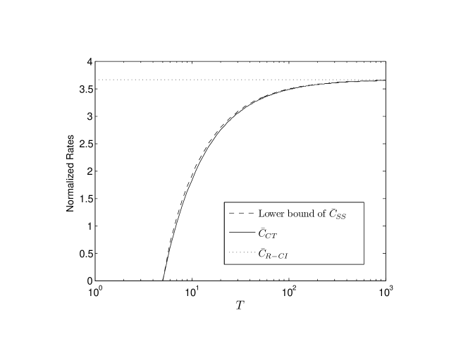
Figure 4: Here we fix an $H$ with $M=5$ over binary field. We plot the lower bounds for $T$ from $5$ to $1000$.

The gap between the lower bound of $\bar{C}_{\text{SS}}(H,T)$ and $\bar{C}_{\text{CT}}(H,T)$ is quit small, which is demonstrated in Fig. 4. Prop. 4, however, is trivial for $T\leq M$. We can use the similar method in extended channel training to obtain a better lower bound. We can foresee that the improved lower bound of $\bar{C}_{\text{SS}}(H,T)$ is close to $\bar{C}_{\text{ECT}}(H,T)$. We will not repeat the procedure here.

VI-E Proofs

Proof:

Let $\mathcal{U}=\operatorname{Pj}(\mathbb{F}^{T})$. We have

$$I(X;Y) =\sum_{\mathbf{X},\mathbf{Y}}p_{X,Y}(\mathbf{X},\mathbf{Y})\log_{2}\frac{p_{X,Y}(\mathbf{X},\mathbf{Y})}{p_{X}(\mathbf{X})p_{Y}(\mathbf{Y})}$$

$$=\sum_{V,U\in\mathcal{U}}\sum_{\begin{subarray}{c}\mathbf{X},\mathbf{Y}:\\ \langle\mathbf{X}\rangle=U,\langle\mathbf{Y}\rangle=V\end{subarray}}p(\mathbf{X},\mathbf{Y})\log_{2}\frac{p(\mathbf{X},\mathbf{Y})}{p_{X}(\mathbf{X})p_{Y}(\mathbf{Y})}$$

$$\stackrel{{\scriptstyle\text{(a)}}}{{\leq}}\sum_{V,U\in\mathcal{U}}p_{\langle X\rangle\langle Y\rangle}(U,V)\log_{2}\frac{p_{\langle X\rangle\langle Y\rangle}(U,V)}{p_{\langle X\rangle}(U)p_{\langle Y\rangle}(V)}$$

$$=I(\langle X\rangle;\langle Y\rangle),$$

where (a) follows from the log-sum inequality. To prove this proposition, we only need to show the equality in (a) holds for uniform LOCs. We need to check that $P_{Y|X}(\mathbf{Y}|\mathbf{X})/p_{Y}(\mathbf{Y})$ is a constant for all $\mathbf{X}$ and $\mathbf{Y}$ with $\langle\mathbf{Y}\rangle=V\leq\langle\mathbf{X}\rangle=U\leq\mathbb{F}^{T}$. Fix an input distribution $p_{X}$. Since the LOC is uniform,

$$p_{Y}(\mathbf{Y}) =\sum_{\mathbf{X}:V\leq\langle\mathbf{X}\rangle}P_{Y|X}(\mathbf{Y}|\mathbf{X})p_{X}(\mathbf{X})$$

$$=\sum_{U^{\prime}\leq\mathbb{F}^{T}:V\leq U^{\prime}}\mu(U,V)\sum_{\mathbf{X}:\langle\mathbf{X}\rangle=U^{\prime}}p_{X}(\mathbf{X})$$

$$=\sum_{U^{\prime}\leq\mathbb{F}^{T}:V\leq U^{\prime}}\mu(U^{\prime},V)p_{\langle X\rangle}(U^{\prime}).$$

Thus,

$$\frac{P_{Y|X}(\mathbf{Y}|\mathbf{X})}{p_{Y}(\mathbf{Y})} =\frac{\mu(U,V)}{\sum_{U^{\prime}\leq\mathbb{F}^{T}:V\leq U^{\prime}}\mu(U^{\prime},V)p_{\langle X\rangle}(U^{\prime})}.$$

This verifies the equality in (a) holding. ∎

Proof:

Fix an $\alpha$-type input $p_{X}$. For $V\leq U\leq\mathbb{F}^{T}$ with $\dim(U)=r$ and $\dim(V)=s$, we first show

$$p_{\langle X\rangle\langle Y\rangle}(U,V)=\frac{p_{\operatorname{\text{rk}}(X)\operatorname{\text{rk}}(Y)}(r,s)}{\left({}^{T}_{r}\right)_{q}\left({}^{r}_{s}\right)_{q}}.$$ (19)

We only need to show that $p_{\langle X\rangle\langle Y\rangle}(U,V)=p_{\langle X\rangle\langle Y\rangle}(U^{\prime},V^{\prime})$ for any $V\leq U\leq\mathbb{F}^{T}$ and $V^{\prime}\leq U^{\prime}\leq\mathbb{F}^{T}$ with $\dim(U)=\dim(U^{\prime})$ and $\dim(V)=\dim(V^{\prime})$, because if this is true,

$$p_{\operatorname{\text{rk}}(X)\operatorname{\text{rk}}(Y)}(r,s) =\sum_{\dim(U^{*})=r,\dim(V^{*})=s,V^{*}\subset U^{*}}p_{\langle X\rangle\langle Y\rangle}(U^{*},V^{*})$$

$$=p_{\langle X\rangle\langle Y\rangle}(U,V)\sum_{\dim(U^{*})=r,\dim(V^{*})=s,V^{*}\subset U^{*}}1$$

$$=p_{\langle X\rangle\langle Y\rangle}(U,V)\begin{pmatrix}T\\ r\end{pmatrix}_{q}\begin{pmatrix}r\\ s\end{pmatrix}_{q}.$$

Let

$$A(m,U)=\{\mathbf{X}\in\mathbb{F}^{t\times m}:\langle\mathbf{X}\rangle=U\}.$$

By Lemma 18, we can find $\Phi\in\operatorname{Fr}(\mathbb{F}^{T\times T})$ such that $\Phi U=U^{\prime}$ and $\Phi V=V^{\prime}$. Then,

$$p_{\langle X\rangle\langle Y\rangle}(U,V) ={\sum_{\mathbf{X}\in A(M,U)}p_{X}(\mathbf{X})\sum_{\mathbf{Y}\in A(N,V)}P_{Y|X}(\mathbf{Y}|\mathbf{X})}$$

$$\stackrel{{\scriptstyle\text{(b)}}}{{=}}{\sum_{\mathbf{X}\in A(M,U)}p_{X}(\Phi\mathbf{X})\sum_{\mathbf{Y}\in A(N,V)}P_{Y|X}(\Phi\mathbf{Y}|\Phi\mathbf{X})}$$

$$\stackrel{{\scriptstyle\text{(c)}}}{{=}}{\sum_{\mathbf{X}\in A(M,\Phi U)}p_{X}(\mathbf{X})\sum_{\mathbf{Y}\in A(N,\Phi V)}P_{Y|X}(\mathbf{Y}|\mathbf{X})}$$

$$=p_{\langle X\rangle\langle Y\rangle}(\Phi U,\Phi V)$$

$$=p_{\langle X\rangle\langle Y\rangle}(U^{\prime},V^{\prime}).$$

(b) follows that $p_{X}$ is $\alpha$-type ($p_{X}(\mathbf{X})=p_{X}(\Phi\mathbf{X})$) and $P_{Y|X}(\Phi\mathbf{Y}|\Phi\mathbf{X})=P_{Y|X}(\mathbf{Y}|\mathbf{X})$ follows from Cor. 4. (c) follows from $A(m,\Phi U)=\Phi A(m,U)$ (see Lemma 20). This proves (19).

Applying the property of $\alpha$-type input,

$$p_{\langle X\rangle}(U) =\sum_{\mathbf{X}\in A(M,U)}p_{X}(\mathbf{X})$$

$$=\sum_{\mathbf{X}\in A(M,U)}p_{X}(\Phi\mathbf{X})$$

$$=\sum_{\mathbf{X}\in\Phi A(M,U)}p_{X}(\mathbf{X})$$

$$\stackrel{{\scriptstyle\text{(d)}}}{{=}}\sum_{\mathbf{X}\in A(M,U^{\prime})}p_{X}(\mathbf{X})$$

$$=p_{\langle X\rangle}(U^{\prime})$$

where (d) follows from Lemma 20). Therefore,

$$p_{\langle X\rangle}(U)=\frac{p_{\operatorname{\text{rk}}(X)}(r)}{\left({}^{T}_{r}\right)_{q}}.$$ (20)

Moreover,

$$p_{\langle Y\rangle}(V) =\sum_{U:V\subset U}p_{\langle X\rangle\langle Y\rangle}(U,V)$$

$$=\sum_{r\geq s}\sum_{U:V\subset U,\dim(U)=r}p_{\langle X\rangle\langle Y\rangle}(U,V)$$

$$=\sum_{r\geq s}\frac{p_{\operatorname{\text{rk}}(X)\operatorname{\text{rk}}(Y)}(r,s)}{\left({}^{T}_{r}\right)_{q}\left({}^{r}_{s}\right)_{q}}\sum_{U:V\subset U,\dim(U)=r}1$$

$$\stackrel{{\scriptstyle\text{(e)}}}{{=}}\sum_{r\geq s}\frac{p_{\operatorname{\text{rk}}(X)\operatorname{\text{rk}}(Y)}(r,s)}{\left({}^{T}_{r}\right)_{q}\left({}^{r}_{s}\right)_{q}}\begin{pmatrix}T-s\\ r-s\end{pmatrix}_{q}$$

$$\stackrel{{\scriptstyle\text{(f)}}}{{=}}\sum_{r\geq s}\frac{p_{\operatorname{\text{rk}}(X)\operatorname{\text{rk}}(Y)}(r,s)}{\left({}^{T}_{r}\right)_{q}\left({}^{r}_{s}\right)_{q}}\begin{pmatrix}T\\ r\end{pmatrix}_{q}\frac{\chi^{r}_{s}}{\chi^{T}_{s}}$$

$$=\frac{p_{\operatorname{\text{rk}}(Y)}(s)}{\left({}^{T}_{s}\right)_{q}},$$ (21)

where (e) and (f) follow from Lemma 14. Substituting (19), (20) and (21) into $I(\langle X\rangle;\langle Y\rangle)$, we have

$$I(\langle X\rangle;\langle Y\rangle)$$

$$= \sum_{V\leq U}p_{\langle X\rangle\langle Y\rangle}(U,V)\log_{2}\frac{p_{\langle X\rangle\langle Y\rangle}(U,V)}{p_{\langle X\rangle}(U)p_{\langle Y\rangle}(V)}$$

$$= \sum_{s\leq r}\sum_{\begin{subarray}{c}V\leq U,\dim(U)=r,\\ \dim(V)=s\end{subarray}}p_{\langle X\rangle\langle Y\rangle}(U,V)\log_{2}\frac{p_{\langle X\rangle\langle Y\rangle}(U,V)}{p_{\langle X\rangle}(U)p_{\langle Y\rangle}(V)}$$

$$= \sum_{s\leq r}\sum_{\begin{subarray}{c}V\leq U,\dim(U)=r,\\ \dim(V)=s\end{subarray}}p_{\langle X\rangle\langle Y\rangle}(U,V)\log_{2}\frac{p_{\operatorname{\text{rk}}(X)\operatorname{\text{rk}}(Y)}(r,s)}{p_{\operatorname{\text{rk}}(X)}(r)p_{\operatorname{\text{rk}}(Y)}(s)}\frac{\left({}^{T}_{s}\right)_{q}}{\left({}^{r}_{s}\right)_{q}}$$

$$= \sum_{s\leq r}p_{\operatorname{\text{rk}}(X)\operatorname{\text{rk}}(Y)}(s,r)\log_{2}\frac{p_{\operatorname{\text{rk}}(X)\operatorname{\text{rk}}(Y)}(r,s)}{p_{\operatorname{\text{rk}}(X)}(r)p_{\operatorname{\text{rk}}(Y)}(s)}\frac{\left({}^{T}_{s}\right)_{q}}{\left({}^{r}_{s}\right)_{q}}$$

$$= I(\operatorname{\text{rk}}(X);\operatorname{\text{rk}}(Y))+\sum_{s\leq r}p_{\operatorname{\text{rk}}(X)\operatorname{\text{rk}}(Y)}(r,s)\log_{2}\frac{\chi^{T}_{s}}{\chi^{r}_{s}}.$$

This completes the proof. ∎

Proof:

Substituting the $\alpha$-type input with $p_{\operatorname{\text{rk}}(X)}(M)=1$ in Lemma 4, we have $I(\operatorname{\text{rk}}(X);\operatorname{\text{rk}}(Y))=0$ and $J(\operatorname{\text{rk}}(X);\operatorname{\text{rk}}(Y))=\sum_{s}P_{\operatorname{\text{rk}}(Y)|\operatorname{\text{rk}}(X)}(s|M)\log_{2}\frac{\chi^{T}_{s}}{\chi^{M}_{s}}$. Given $\mathbf{X}\in\mathbb{F}^{T\times M}$ with dimension $M$,

$$P_{\operatorname{\text{rk}}(Y)|X}(s|\mathbf{X})=\Pr\{\operatorname{\text{rk}}(\mathbf{X}H)=s\}=\Pr\{\operatorname{\text{rk}}(H)=s\}.$$

Thus, $P_{\operatorname{\text{rk}}(Y)|\operatorname{\text{rk}}(X)}(s|M)=\Pr\{\operatorname{\text{rk}}(H)=s\}$. Using the definition in (3), we can write

$$\log_{2}\frac{\chi^{T}_{s}}{\chi^{M}_{s}} =\log_{2}\frac{\zeta^{T}_{s}q^{Ts}}{\zeta^{M}_{s}q^{Ms}}$$

$$=(T-M)s\log_{2}q+\log_{2}\frac{\zeta^{T}_{s}}{\zeta^{M}_{s}}.$$

Since $\zeta^{T}_{s}<1$,

$$\log_{2}\frac{\zeta^{T}_{s}}{\zeta^{M}_{s}}<\log_{2}\frac{1}{\zeta^{M}_{s}}<1.8,$$ (22)

where the last inequality follows from Lemma 15. So

$$J(\operatorname{\text{rk}}(X);\operatorname{\text{rk}}(Y)) =\sum_{s}p_{\operatorname{\text{rk}}(H)}(s)(T-M)s\log_{2}q+$$

$$\quad\sum_{s}p_{\operatorname{\text{rk}}(H)}(s)\log_{2}\frac{\zeta^{T}_{s}}{\zeta^{M}_{s}}$$

$$=(T-M)\log_{2}q\operatorname{E}[\operatorname{\text{rk}}(H)]+\epsilon(T,q)T\log_{2}q,$$

where $\epsilon(T,q)=\sum_{s}p_{\operatorname{\text{rk}}(H)}(s)\log_{2}\frac{\zeta^{T}_{s}}{\zeta^{M}_{s}}/(T\log_{2}q)<1.8/(T\log_{2}q)$. The proof is complete by $C_{\text{SS}}(H,T)\geq J(\operatorname{\text{rk}}(X);\operatorname{\text{rk}}(Y))$. ∎

VII Optimal Inputs for Subspace Coding

In this section, we show that using constant-dimensional subspace coding is almost as good as the general (multi-dimensional) subspace coding.

VII-A A Formulation of $\alpha$-type Inputs

Lemma 5

A function $p:\mathbb{F}^{T\times M}\rightarrow\mathbb{R}$ is an $\alpha$-type PMF if and only if it can be written as

$$p(\mathbf{X})=R(\operatorname{\text{rk}}(\mathbf{X}))\frac{Q_{\operatorname{\text{rk}}(\mathbf{X})}(\langle\mathbf{X}^{\top}\rangle)}{\chi^{T}_{\operatorname{\text{rk}}(\mathbf{X})}}$$ (23)

where $Q_{r}(\cdot)$ is a PMF over $\operatorname{Gr}(r,\mathbb{F}^{M})$ and $R(\cdot)$ be a PMF over $\{0,1,\cdots,M\}$.

Proof:

If $p$ can be written as (23), by Lemma 1, $p$ is an $\alpha$-type PMF. On the other hand, if $p$ is an $\alpha$-type PMF, it can be written as (12). Let

$$R(r)=\sum_{\tilde{U}:\operatorname{\text{rk}}(\tilde{U})=r}Q(\tilde{U}).$$

For $r$ such that $R(r)>0$, let

$$Q_{r}(\tilde{U})=\left\{\begin{array}[]{ll}Q(\tilde{U})/R(r)&\dim(\tilde{U})=r\\ 0&o.w..\end{array}\right.$$

For $r$ such that $R(r)=0$, let $Q_{r}(\cdot)$ be any PMF over $\operatorname{Gr}(r,\mathbb{F}^{M})$. Since $Q_{\dim(\tilde{U})}(\tilde{U})R(\dim(\tilde{U}))=Q(\tilde{U})$, we see that $p$ can be written as (23). ∎

When using the formulation in (23), $I(\operatorname{\text{rk}}(X);\operatorname{\text{rk}}(Y))$ and $J(\operatorname{\text{rk}}(X);\operatorname{\text{rk}}(Y))$ can be written as functions of $Q_{r}(\tilde{U})$ and $R(r)$ as follows. Using the property of Markov chain,

$$P_{\operatorname{\text{rk}}(Y)|\operatorname{\text{rk}}(X)}(s|r)$$

$$=\sum_{\tilde{U}\in\operatorname{Gr}(r,\mathbb{F}^{M})}P_{\operatorname{\text{rk}}(Y)|\langle X^{\top}\rangle}(s|\tilde{U})P_{\langle X^{\top}\rangle|\operatorname{\text{rk}}(X)}(\tilde{U}|r)$$

$$=\sum_{\tilde{U}\in\operatorname{Gr}(r,\mathbb{F}^{M})}P_{\operatorname{\text{rk}}(Y)|\langle X^{\top}\rangle}(s|\tilde{U})Q_{r}(\tilde{U}),$$ (24)

in which $P_{\operatorname{\text{rk}}(Y)|\langle X^{\top}\rangle}(s|\tilde{U})$, given in Coro. 3, is a function of $p_{H}$ and is not related to $Q_{r}(\tilde{U})$ and $R(r)$. Thus, we can write

$${I(\operatorname{\text{rk}}(X);\operatorname{\text{rk}}(Y))}=\sum_{r}R(r)\sum_{s}P(s|r)\log_{2}\frac{P(s|r)}{\sum_{r^{\prime}}P(s|r^{\prime})R(r^{\prime})},$$ (25)

in which $P(s|r)=P_{\operatorname{\text{rk}}(Y)|\operatorname{\text{rk}}(X)}(s|r)$ is given in (24); and

$${J}(\operatorname{\text{rk}}(X);\operatorname{\text{rk}}(Y)) =\sum_{r}R(r)\sum_{\tilde{U}\in\operatorname{Gr}(r,\mathbb{F}^{M})}Q_{r}(\tilde{U})g(\tilde{U}),$$

in which

$$g(\tilde{U})\triangleq\sum_{s}P_{\operatorname{\text{rk}}(Y)|\langle X^{\top}\rangle}(s|\tilde{U})\log_{2}\frac{\chi^{T}_{s}}{\chi^{\dim(\tilde{U})}_{s}}.$$ (26)

Note that $g(\tilde{U})$ only depends on the distribution of $H$, but does not depend on the input. Define

$$\operatorname{\text{rk}}^{*}(H)=\max\{r:\Pr\{\operatorname{\text{rk}}(H)=r\}>0\},$$

i.e., the maximum nonzero rank of the transformation matrix.

Lemma 6

Consider $\text{LOC}(H,T)$ with dimension $M\times N$ and $T\geq M$. Fix an $\alpha$-type input. For $\tilde{V}\leq\mathbb{F}^{M}$ with $\dim(\tilde{V})=r<\operatorname{\text{rk}}^{*}(H)$,

$$g(\mathbb{F}^{M})-g(\tilde{V})>\Theta(T,r,H)\log_{2}q,$$

where

$$\Theta(T,r,H) =(T-M)(\operatorname{\text{rk}}^{*}(H)-r)p_{\operatorname{\text{rk}}(H)}(\operatorname{\text{rk}}^{*}(H))$$

$$\qquad-r(M-r)+\log_{q}\zeta^{r}_{r}.$$

Proof:

See §VII-E. ∎

VII-B Optimal Inputs for Subspace Coding

We treat $Q_{r}(\mathbf{X})$ and $R(r)$ as the variables to maximize $I(\langle X\rangle;\langle Y\rangle)$. By the KKT conditions, a set of necessary and sufficient conditions such that an $\alpha$-type input with variables $Q_{r}(\mathbf{X})$ and $R(r)$ to achieve $C_{\text{SS}}(H,T)$ is that

$$\frac{\partial I(\operatorname{\text{rk}}(X);\operatorname{\text{rk}}(Y))}{\partial Q_{r}(\tilde{U})} +R(r)g(\tilde{U})=\lambda_{r}$$

$$\forall r,\tilde{U}\in\operatorname{Gr}(r,\mathbb{F}^{M}):Q_{r}(\tilde{U})>0,$$ (27a)

$$\frac{\partial I(\operatorname{\text{rk}}(X);\operatorname{\text{rk}}(Y))}{\partial Q_{r}(\tilde{U})} +R(r)g(\tilde{U})\leq\lambda_{r}$$

$$\forall r,\tilde{U}\in\operatorname{Gr}(r,\mathbb{F}^{M}):Q_{r}(\tilde{U})=0,$$ (27b)

$$\frac{\partial I(\operatorname{\text{rk}}(X);\operatorname{\text{rk}}(Y))}{\partial R(r)} +\sum_{\tilde{U}\in\operatorname{Gr}(r,\mathbb{F}^{M})}Q_{r}(\tilde{U})g(\tilde{U})=\bar{\lambda}$$

$$\forall r:R(r)>0,$$ (27c)

$$\frac{\partial I(\operatorname{\text{rk}}(X);\operatorname{\text{rk}}(Y))}{\partial R(r)} +\sum_{\tilde{U}\in\operatorname{Gr}(r,\mathbb{F}^{M})}Q_{r}(\tilde{U})g(\tilde{U})\leq\bar{\lambda}$$

$$\forall r:R(r)=0,$$ (27d)

where the partial derivatives are

$$\frac{\partial I(\operatorname{\text{rk}}(X);\operatorname{\text{rk}}(Y))}{\partial Q_{r}(\tilde{U})}$$

$$=R(r)\sum_{s}P_{\operatorname{\text{rk}}(Y)|\langle X^{\top}\rangle}(s|\tilde{U})\log_{2}\frac{P_{\operatorname{\text{rk}}(Y)|\operatorname{\text{rk}}(X)}(s|r)}{P_{\operatorname{\text{rk}}(Y)}(s)}-\log_{2}e,$$

and

$$\frac{\partial I(\operatorname{\text{rk}}(X);\operatorname{\text{rk}}(Y))}{\partial R(r)}$$

$$=\sum_{s}P_{\operatorname{\text{rk}}(Y)|\operatorname{\text{rk}}(X)}(s|r)\log_{2}\frac{P_{\operatorname{\text{rk}}(Y)|\operatorname{\text{rk}}(X)}(s|r)}{P_{\operatorname{\text{rk}}(Y)}(s)}-\log_{2}e.$$

We can check that

$$C_{\text{SS}}(H,T)=\lambda+\log_{2}e,$$

and

$$\lambda=\sum_{r}\lambda_{r}+(M-1)\log_{2}e.$$

The above optimization problem to find an optimal input for subspace coding is in general hard. We have already shown that for large $T$, the $M$-dimensional $\alpha$-type input gives a good approximation of the channel capacity (see Prop. 4). Here, we can further improve the result for a class of LOCs

Definition 4

A random matrix $H$ with dimension $M\times N$ is regular if $p_{\operatorname{\text{rk}}(H)}(s)>0$ for $0\leq s\leq M$. $\text{LOC}(H,T)$ is regular if $H$ is regular.

Theorem 5

Consider regular $\text{LOC}(H,T)$ with dimension $M\times N$. There exists $T_{1}$ such that when $T\geq T_{1}$, $C_{\text{SS}}$ is achieved by the $\alpha$-type input with $R(M)=1$. In this case $C_{\text{SS}}(H,T)=g(\mathbb{F}^{M})=\sum_{s}p_{\operatorname{\text{rk}}(H)}(s)\log_{2}\frac{\chi^{T}_{s}}{\chi^{M}_{s}}=\operatorname{E}\left[\log_{2}\frac{\chi^{T}_{\operatorname{\text{rk}}(H)}}{\chi^{M}_{\operatorname{\text{rk}}(H)}}\right]$.

Proof:

See §VII-E. ∎

Assume $M\leq N$. Since $p_{\operatorname{\text{rk}}(H_{\text{pure}})}(r)=\chi^{M,N}_{r}q^{-MN}$ for $r\leq M$, $H_{\text{pure}}$ is regular.

VII-C Optimal Constant-Rank Inputs

An input for a LOC with $p_{\operatorname{\text{rk}}(X)}(r)=1$ is called a constant-rank or rank-$r$ input distribution. When talking about subspace coding, rank-$r$ input is corresponding to $r$-dimensional subspace coding. Our discussion of constant-rank inputs for subspace coding is equivalent to the discussion of constant-dimensional subspace coding.

Let

$$C_{\text{C-SS}}(H,T)=\max_{p_{X}:\text{constant-rank}}I(\langle X\rangle;\langle Y\rangle)$$

so that $C_{\text{C-SS}}(H,T)$ is the maximum achievable rates of constant-dimensional subspace coding. Let $\bar{C}_{\text{C-SS}}(H,T)$ be the normalization of $C_{\text{C-SS}}(H,T)$ by $T\log_{2}q$. The rank of a constant-rank input that achieves $C_{\text{C-SS}}(H,T)$ is called an optimal input rank. We show that to find an optimal input rank, we only need to consider $\alpha$-type inputs. Moreover, we can determine $C_{\text{C-SS}}(H,T)$ and an optimal input rank based on sufficient channel statistics such that we can calculate $g(\tilde{U})$. See Prop. 6 and Theorem 7 for details.

Theorem 6

For any LOCs, there exists a constant-rank $\alpha$-type input that achieves $C_{\text{C-SS}}(H,T)$.

Proof:

The proof is similar to the proof of Proposition 2. See §VII-E. ∎

Theorem 7

For $\text{LOC}(H,T)$ with dimension $M\times N$, let

$$U^{*}=\arg\max_{\tilde{U}\in\operatorname{Pj}(M^{*},\mathbb{F}^{M})}g(\tilde{U}).$$

Then, $r^{*}=\dim(\tilde{U}^{*})$ is an optimal input rank and $C_{\text{C-SS}}(H,T)=g(\tilde{U}^{*})$. Furthermore,

$$\bar{C}_{\text{SS}}(H,T)-\bar{C}_{\text{C-SS}}(H,T)\leq\frac{\log_{2}\min\{M,N\}}{T\log_{2}q}.$$

Proof:

See §VII-E. ∎

Theorem 7 also bounds the loss of rate when using constant-dimensional subspace coding. Assume $M=N=5$, $T=10$, $q=4$ and $\operatorname{E}[\operatorname{\text{rk}}(H)]=M/4$. We have

$$\frac{\bar{C}_{\text{SS}}(H,T)-\bar{C}_{\text{C-SS}}(H,T)}{\bar{C}_{\text{SS}}(H,T)} <\frac{\log_{2}M}{T\log_{2}q(1-M/T)\operatorname{E}[\operatorname{\text{rk}}(H)]}$$

$$=9.8\$$

So the loss of rate is marginal for typical channel parameters.

VII-D Optimal Input Rank

To evaluate the results in Theorems 6 and Theorem 7, we require the distribution of the transformation matrix. Now we show that in some cases, we can relax this requirement significantly. For $\text{LOC}(H,T)$, recall that

$$\operatorname{\text{rk}}^{*}(H)=\max\{r:\Pr\{\operatorname{\text{rk}}(H)=r\}>0\}.$$

Theorem 8

For $\text{LOC}(H,T)$, there exists $T_{0}$ such that when $T\geq T_{0}$, $r^{*}\geq\operatorname{\text{rk}}^{*}(H)$, where $r^{*}$ is the optimal input rank given in Theorem 7.

Proof:

Suppose the dimension of the LOC is $M\times N$. Fix $T_{0}$ such that $\Theta(T_{0},r,H)\geq 0$ for all $r<\operatorname{\text{rk}}^{*}(H)$. This is possible because $\Theta(T,r,H)$ is a linearly increase function of $T$ for all $r<\operatorname{\text{rk}}^{*}(H)$. Assume $T\geq T_{0}$ and $r^{*}<\operatorname{\text{rk}}^{*}(H)$. For any $\tilde{V}\leq\mathbb{F}^{M}$ with $\dim(\tilde{V})<\operatorname{\text{rk}}^{*}(H)\leq M$, by Lemma 6,

$$g(\mathbb{F}^{M})>g(\tilde{V}).$$

Thus, we have a contradiction to $r^{*}<\operatorname{\text{rk}}^{*}(H)$. ∎

Theorem 8 narrows down the range to search an optimal input rank for large $T$. When $\operatorname{\text{rk}}^{*}(H)=M$, it tells that $M$ is an optimal input rank when $T$ is sufficiently large. The proof of Theorem 8 tells how to find a $T_{0}$.

As an example, let us check the optimal input rank of $\text{LOC}(H_{\text{full}},T)$. We know $\operatorname{\text{rk}}^{*}(H_{\text{full}})=M$ and $p_{\operatorname{\text{rk}}(H_{\text{full}})}(M)=1$. By Theorem 8, there exists $T_{0}$ such that when $T>T_{0}$, $r^{*}=M$. Now we want to know the value of $T_{0}$. From the proof of Theorem 8, we know that $T_{0}$ should satisfy

$$\Theta(T_{0},r,H_{\text{full}})\geq 0,\quad\forall r<M.$$

In other words, $T_{0}$ should satisfy

$$(r-T_{0}/2)^{2}-(T_{0}/2-M)^{2}+\log_{q}\zeta^{r}_{r}\geq 0,\quad\forall r<M.$$ (28)

If $M\leq T_{0}\leq 2M-1$, (28) does not hold for $r=M-1$. If $T_{0}=2M$, the minimum value of the RHS of (28) is obtained for $r=M-1$, i.e., $1+\log_{q}\zeta^{M}_{M}$, which is positive when $q>2$. Similarly, we can check that $T_{0}=2M+1$ is sufficient for any field size. As a conclusion, when i) $q>2$ and $T\geq 2M$ or ii) $q=2$ and $T\geq 2M+1$, the $M$-dimensional $\alpha$-type input is an optimal constant-rank input for $(H_{\text{full}},T)$.

VII-E proofs

Proof:

Let $\tilde{U}=\mathbb{F}^{M}$. Since $\tilde{V}\leq\tilde{U}$, we can find a full rank $M\times M$ matrix

$$\mathbf{D}=\begin{bmatrix}\mathbf{D}_{0}\\ \mathbf{D}_{1}\end{bmatrix}$$

such that $\langle\mathbf{D}^{\top}\rangle=\tilde{U}$ and $\langle\mathbf{D}_{1}^{\top}\rangle=\tilde{V}$. By Coro. 3,

$$\sum_{s^{\prime}\geq s}P_{\operatorname{\text{rk}}(Y)|\langle X^{\top}\rangle}(s^{\prime}|\tilde{V}) =\Pr\{\operatorname{\text{rk}}(\mathbf{D_{1}}H)\geq s\},$$

and

$$P_{\operatorname{\text{rk}}(Y)|\langle X^{\top}\rangle}(s|\tilde{U}) =\Pr\{\operatorname{\text{rk}}(\mathbf{D}H)=s\}$$

$$=\Pr\{\operatorname{\text{rk}}(H)=s\}.$$

We know $\Pr\{\operatorname{\text{rk}}(H)\geq s\}\geq\Pr\{\operatorname{\text{rk}}(\mathbf{D_{1}}H)\geq s\}$. So

$$\sum_{s^{\prime}\geq s}P_{\operatorname{\text{rk}}(Y)|\langle X^{\top}\rangle}(s^{\prime}|\tilde{U})\geq\sum_{s^{\prime}\geq s}P_{\operatorname{\text{rk}}(Y)|\langle X^{\top}\rangle}(s^{\prime}|\tilde{V}).$$

Moreover, for $s$ such that $r<s\leq\operatorname{\text{rk}}^{*}(H)$,

$$\sum_{s^{\prime}\geq s}P_{\operatorname{\text{rk}}(Y)|\langle X^{\top}\rangle}(s^{\prime}|\tilde{V})=0.$$

Thus,

$$\sum_{s}s(P_{\operatorname{\text{rk}}(Y)|\langle X^{\top}\rangle}(s|\tilde{U})-P_{\operatorname{\text{rk}}(Y)|\langle X^{\top}\rangle}(s|\tilde{V}))$$

$$=\sum_{k}\sum_{s\geq k}(P_{\operatorname{\text{rk}}(Y)|\langle X^{\top}\rangle}(s|\tilde{U})-P_{\operatorname{\text{rk}}(Y)|\langle X^{\top}\rangle}(s|\tilde{V}))$$

$$\geq\sum_{k:\operatorname{\text{rk}}^{*}(H)\geq k>r}\sum_{s:s\geq k}P_{\operatorname{\text{rk}}(Y)|\langle X^{\top}\rangle}(s|\tilde{U})$$

$$\geq\sum_{k:\operatorname{\text{rk}}^{*}(H)\geq k>r}\Pr\{\operatorname{\text{rk}}(H)=\operatorname{\text{rk}}^{*}(H)\}$$

$$=(\operatorname{\text{rk}}^{*}(H)-r)\Pr\{\operatorname{\text{rk}}(H)=\operatorname{\text{rk}}^{*}(H)\}.$$ (29)

By definition,

$$\frac{g(\tilde{U})-g(\tilde{V})}{\log_{2}q}$$

$$=\sum_{s}P_{\operatorname{\text{rk}}(Y)|\langle X^{\top}\rangle}(s|\tilde{U})\left((T-M)s+\log_{q}\frac{\zeta^{T}_{s}}{\zeta^{M}_{s}}\right)$$

$$\qquad-\sum_{s}P_{\operatorname{\text{rk}}(Y)|\langle X^{\top}\rangle}(s|\tilde{V})\left((T-r)s+\log_{q}\frac{\zeta^{T}_{s}}{\zeta^{r}_{s}}\right)$$

$$=(T-M)\sum_{s}s(P_{\operatorname{\text{rk}}(Y)|\langle X^{\top}\rangle}(s|\tilde{U})-P_{\operatorname{\text{rk}}(Y)|\langle X^{\top}\rangle}(s|\tilde{V}))$$

$$\qquad-(M-r)\sum_{s}sP_{\operatorname{\text{rk}}(Y)|\langle X^{\top}\rangle}(s|\tilde{V})$$

$$\qquad+\sum_{s}P_{\operatorname{\text{rk}}(Y)|\langle X^{\top}\rangle}(s|\tilde{U})\log_{q}\frac{\zeta^{T}_{s}}{\zeta^{M}_{s}}$$

$$\qquad-\sum_{s}P_{\operatorname{\text{rk}}(Y)|\langle X^{\top}\rangle}(s|\tilde{V})\log_{q}\frac{\zeta^{T}_{s}}{\zeta^{r}_{s}}$$

$$>(T-M)(\operatorname{\text{rk}}^{*}(H)-r)\Pr\{\operatorname{\text{rk}}(H)=\operatorname{\text{rk}}^{*}(H)\}$$

$$\qquad-r(M-r)+\log_{q}\zeta^{r}_{r},$$

where the last inequality follows from (29). Therefore

$$(M-r)\sum_{s}sP_{\operatorname{\text{rk}}(Y)|\langle X^{\top}\rangle}(s|\tilde{V})\leq r(M-r),$$

$$\sum_{s}P_{\operatorname{\text{rk}}(Y)|\langle X^{\top}\rangle}(s|\tilde{U})\log_{q}\frac{\zeta^{T}_{s}}{\zeta^{M}_{s}}\geq 0,$$

and

$$\sum_{s}P_{\operatorname{\text{rk}}(Y)|\langle X^{\top}\rangle}(s|\tilde{V})\log_{q}\frac{\zeta^{T}_{s}}{\zeta^{r}_{s}}<\sum_{s}P_{\operatorname{\text{rk}}(Y)|\langle X^{\top}\rangle}(s|\tilde{V})\log_{q}\frac{1}{\zeta^{r}_{s}}\leq\log_{q}\frac{1}{\zeta^{r}_{r}}.$$

∎

Proof:

To prove the theorem, we only need to check that the $\alpha$-type input with $R(M)=1$ satisfies (27). Conditions (27a) and (27b) with $r<M$ are satisfied by $\lambda_{r}=\log_{2}e$ because $R(r)=0$. Since $Q_{M}(\mathbb{F}^{M})=1$, we check condition (27a) with $r=M$. Since $P_{\operatorname{\text{rk}}(Y)|\operatorname{\text{rk}}(X)}(s|M)=P_{\operatorname{\text{rk}}(Y)}(s)$,

$$\left.\frac{\partial I(\operatorname{\text{rk}}(X);\operatorname{\text{rk}}(Y))}{\partial Q_{M}(\mathbb{F}^{M})}\right|_{R(M)=1}=-\log_{2}e.$$

So, (27a) with $r=M$ is satisfied by $\lambda_{M}=g(\mathbb{F}^{M})-\log_{2}e$. This completes the verification of (27a) and (27b).

The above analysis also tells that $\bar{\lambda}=\lambda_{M}$. Now we check (27c) and (27d) with $\bar{\lambda}=g(\mathbb{F}^{M})-\log_{2}e$. Since $R(M)=1$, condition (27c) should be satisfied with $r=M$. This is true since

$$\left.\frac{\partial I(\operatorname{\text{rk}}(X);\operatorname{\text{rk}}(Y))}{\partial R(M)}\right|_{R(M)=1}+g(\mathbb{F}^{M})=-\log_{2}e+g(\mathbb{F}^{M}).$$

Next, we check condition (27d) for $r<M$. We know

$$\left.\frac{\partial I(\operatorname{\text{rk}}(X);\operatorname{\text{rk}}(Y))}{\partial R(r)}\right|_{R(M)=1}$$

$$=\underbrace{\sum_{s}P_{\operatorname{\text{rk}}(Y)|\operatorname{\text{rk}}(X)}(s|r)\log_{2}\frac{P_{\operatorname{\text{rk}}(Y)|\operatorname{\text{rk}}(X)}(s|r)}{P_{\operatorname{\text{rk}}(Y)|\operatorname{\text{rk}}(X)}(s|M)}}_{(A)}-\log_{2}e.$$

Since

$$P_{\operatorname{\text{rk}}(Y)|\operatorname{\text{rk}}(X)}(s|M) =P_{\operatorname{\text{rk}}(Y)|\langle X^{\top}\rangle}(s|\mathbb{F}^{M})$$

$$=\Pr\{\operatorname{\text{rk}}(\mathbf{D}H)=s\}$$

$$=\Pr\{\operatorname{\text{rk}}(H)=s\},$$

we have

$$(A) \leq\sum_{s}P_{\operatorname{\text{rk}}(Y)|\operatorname{\text{rk}}(X)}(s|r)\log_{2}\frac{1}{P_{\operatorname{\text{rk}}(Y)|\operatorname{\text{rk}}(X)}(s|M)}$$

$$=\sum_{s}P_{\operatorname{\text{rk}}(Y)|\operatorname{\text{rk}}(X)}(s|r)\log_{2}\frac{1}{p_{\operatorname{\text{rk}}(H)}(s)}$$

$$\leq-\log_{2}\min_{0\leq s<M}p_{\operatorname{\text{rk}}(H)}(s).$$

That is

$$\left.\frac{\partial I(\operatorname{\text{rk}}(X);\operatorname{\text{rk}}(Y))}{\partial R(r)}\right|_{R(M)=1}\leq-\log_{2}\min_{0\leq s\leq M}p_{\operatorname{\text{rk}}(H)}(s)-\log_{2}e.$$

Fix $T_{1}$ such that $\Theta(T_{1},r,H)\geq-\log_{2}\min_{0\leq s<M}p_{\operatorname{\text{rk}}(H)}(s)$ for all $r<M$. This is possible because $\Theta(T,r,H)$ is linearly increase with $T$ and $-\log_{2}\min_{0\leq s<M}p_{\operatorname{\text{rk}}(H)}(s)$ does not change with $T$. By Lemma 6, $g(\mathbb{F}^{M})\geq g(\tilde{U})-\log_{2}\min_{0\leq s\leq M}p_{\operatorname{\text{rk}}(H)}(s)$ for all $\tilde{U}\in\operatorname{Gr}(r,\mathbb{F}^{M})$. Thus

$$\bar{\lambda} =g(\mathbb{F}^{M})-\log_{2}e$$

$$\geq\max_{\tilde{U}\in\operatorname{Gr}(r,\mathbb{F}^{M})}g(\tilde{U})-\log_{2}\min_{0\leq s\leq M}p_{\operatorname{\text{rk}}(H)}(s)-\log_{2}e$$

$$\geq\sum_{\tilde{U}\in\operatorname{Gr}(r,\mathbb{F}^{M})}Q_{r}(\tilde{U})g(\tilde{U})+\left.\frac{\partial I(\operatorname{\text{rk}}(X);\operatorname{\text{rk}}(Y))}{\partial R(r)}\right|_{R(M)=1}.$$

Hence, condition (27d) with $r<M$ is satisfied. ∎

Proof:

Consider a LOC with block length $T$. Let $p_{X}(\mathbf{X})$ be an optimal constant-rank input with $p_{\operatorname{\text{rk}}(X)}(r^{*})=1$. For $\Phi\in\operatorname{Fr}(\mathbb{F}^{T\times T})$, define $p^{\Phi}$ as $p_{X}^{\Phi}(\mathbf{X})=p_{X}(\Phi\mathbf{X})$. It is clear that $p^{\Phi}_{\operatorname{\text{rk}}(X}(r^{*})=1$. By Lemma 2, $p_{X}^{\Phi}(\mathbf{X})$ is also an optimal constant-rank input. Define $p_{X}^{*}$ as

$$p_{X}^{*}(\mathbf{X})=\frac{1}{|\operatorname{Fr}(\mathbb{F}^{T\times T})|}\sum_{\Phi\in\operatorname{Fr}(\mathbb{F}^{T\times T})}p_{X}^{\Phi}(\mathbf{X}).$$

By the concavity of the mutual information, we know $p_{X}^{*}$ is also an optimal constant-rank input. We can check that $p_{X}^{*}$ is $\alpha$-type as in the proof of Proposition 2. ∎

Proof:

For an $r$-dimensional $\alpha$-type input,

$$I(\langle X\rangle;\langle Y\rangle) =\sum_{\tilde{U}\in\operatorname{Gr}(r,\mathbb{F}^{M})}Q_{r}(\tilde{U})g(\tilde{U})$$

$$\leq\max_{\tilde{U}\in\operatorname{Gr}(r,\mathbb{F}^{M})}g(\tilde{U})$$

$$\leq g(\tilde{U}^{*}).$$

Thus $C_{\text{C-SS}}\leq g(\tilde{U}^{*})$. On the other hand, for the $r^{*}$-dimensional $\alpha$-type input with $p_{\langle X^{\top}\rangle}(\tilde{U}^{*})=1$, $C_{\text{C-SS}}\geq I(\langle X\rangle;\langle Y\rangle)=g(\tilde{U}^{*})$.

Furthermore, for an $\alpha$-type input

$$I(\langle X\rangle;\langle Y\rangle)-C_{\text{C-SS}} =I(\operatorname{\text{rk}}(X);\operatorname{\text{rk}}(Y))+J(\operatorname{\text{rk}}{X};\operatorname{\text{rk}}{Y})-g(\tilde{U}^{*})$$

$$\leq I(\operatorname{\text{rk}}(X);\operatorname{\text{rk}}(Y))$$

$$\leq\log_{2}\min\{M,N\}.$$

Thus, $C_{\text{SS}}-C_{\text{C-SS}}=\max_{p_{X}:\alpha-\text{type}}I(\langle X\rangle;\langle Y\rangle)-C_{\text{C-SS}}\leq\log_{2}\min\{M,N\}$. ∎

VIII Coding for Linear Operator Channels

From this section, we consider coding design for $\text{LOC}(H,T)$.

VIII-A Using Channel Training or Subspace Coding

We have considered two kinds of coding schemes for noncoherent LOCs: channel training and subspace coding. For channel training, all the input matrices $\mathbf{X}$ have the form

$$\mathbf{X}=\begin{bmatrix}\mathbf{I}\\ \tilde{\mathbf{X}}\end{bmatrix},$$ (30)

where $\mathbf{I}$ is an identity matrix. For such a transmission, the received matrix

$$\mathbf{Y}=\begin{bmatrix}\mathbf{I}\\ \tilde{\mathbf{X}}\end{bmatrix}\mathbf{H}=\begin{bmatrix}\mathbf{H}\\ \tilde{\mathbf{X}}\mathbf{H}\end{bmatrix},$$

where $\mathbf{H}$ is the instance of $H$. The receiver can use the first part of $\mathbf{Y}$ to recover $\mathbf{H}$ and use this information to decode $\tilde{\mathbf{X}}$. We have shown that the normalized maximum achievable rate using channel training is

$$\bar{C}_{\text{CT}}(H,T)=(1-M/T)\operatorname{E}[\operatorname{\text{rk}}(H)].$$

For subspace coding, a codeword contains a sequence of subspaces and the transmission of a subspace through LOCs involves the transformation of a subspace to a matrix. The decoding also only depends on the subspace spanned by the received matrix. For more details, see our discuss in §VI-B. We have shown that the normalized maximum achievable rate using subspace coding satisfies

$$\operatorname{E}[\operatorname{\text{rk}}(H)]\geq\bar{C}_{\text{SS}}(H,T)\geq(1-M/T)\operatorname{E}[\operatorname{\text{rk}}(H)]+\epsilon(T,q),$$

where $0<\epsilon(T,q)<1.8/(T\log_{2}q)$. We have shown the lower bound of $\bar{C}_{\text{SS}}(H,T)$ is tight for regular LOCs when $T$ is sufficiently large. Therefore

$$\epsilon(T,q)\leq\bar{C}_{\text{SS}}(H,T)-\bar{C}_{\text{CT}}(H,T)<M/T\operatorname{E}[\operatorname{\text{rk}}(H)].$$

So using channel training does not loss much in rates, especially when $T$ is large.

For encoding, a channel training code can be regarded as a special subspace code. But the decoding of channel training codes uses the received matrices, while the decoding of subspace codes uses the subspaces spanned by the received matrices. However, we can just decode a subspace code using the matrices received. If we apply this decoding method of subspace codes, channel training can be regarded as a special case of subspace coding. This is the reason that even some existing subspace coding schemes use channel training [20, 28].

In this paper, we only study the design of channel training codes.

VIII-B Some Existing Channel Training Codes

Existing coding schemes for RLCN also works for LOCs, even though a RLCN is a special LOC with its transformation matrix depends on the network topology. In fact, most coding practice of RLCN is based on channel training. We first introduce two coding schemes for RLCN.

The first coding scheme was introduced by Ho et al.[9]. They assumed that the transformation matrix has rank $M$. In their scheme, a codeword has the form in (30) where any matrix in $\mathbb{F}^{(T-M)\times M}$ can be used as $\tilde{\mathbf{X}}$. We call such codes the classical channel training codes. A received matrix has the form

$$\mathbf{Y}=\begin{bmatrix}\mathbf{I}\\ \tilde{\mathbf{X}}\end{bmatrix}\mathbf{H}=\begin{bmatrix}\mathbf{H}\\ \tilde{\mathbf{X}}\mathbf{H}\end{bmatrix}.$$

Since $\mathbf{H}$ has rank $M$, the receiver can decode $\tilde{\mathbf{X}}$ by solving a system of linear equations. The rateless realization of random linear network codes found in [16, 17] applies a classical channel training code over $\text{LOC}(GH,T)$, where $\text{LOC}(H,T)$ is the original channel and $G$ is an $r\times M$ purely random matrix. We will give a general discussion of this approach and show that we only need to consider $r<M$.

Silva et al. [20] proposed a more general method in which $\tilde{\mathbf{X}}$ in (30) can only be chosen from a rank-metric code. The redundancy in the rank-metric code can be used to correct the rank deficiency of $H$ as well as additive errors, which are not considered in this work. This code construction is nearly optimal in terms of a Singleton type coding bound on one-block subspace codes [19].

Both of the works [9, 20] construct channel training codes with unit block, which in general cannot achieve the channel capacity of LOCs. Two more recent works [27, 28] considers design of channel training codes with non-unit length. The authors proposed a multilevel code construction approach in [27]. Parallel to our work, this approach is used explicitly to construct “multishot rank-metric codes” [27]. Note that the multishot rank-metric codes constructed in [27] is different to the codes we will proposed here, even though we both apply rank metric. For the lack of a performance evaluation of their codes, we cannot see whether their codes achieve $\bar{C}_{\text{CT}}$.

VIII-C Achieve Higher Rate than $\bar{C}_{\text{CT}}$

In the following, we will introduce two constructions of channel training codes for LOCs, called lifted rank-metric codes and lifted linear matrix codes, respectively. We will prove that lifted linear matrix codes can achieve $\bar{C}_{\text{CT}}$. But our codes can also used to achieve higher rate than $\bar{C}_{\text{CT}}$ using extended channel training. The approach is to use $\text{LOC}(H,T)$ as $\text{LOC}(GH,T)$ for any $r\times M$ random matrix $G$. As we discussed in §IV, we only need to consider $r<M$ and Theorem 1 implies that a purely random $G$ is good enough.

VIII-D Formulation of Channel Training Codes

A matrix code $\mathcal{C}^{(n)}\subset\mathbb{F}^{(T-M)\times nM}$ induces a channel training code for $\text{LOC}(H,T)$ with dimension $M\times N$ as follows. For $\tilde{\mathbf{X}}^{(n)}\in\mathcal{C}^{(n)}$, we write

$$\tilde{\mathbf{X}}^{(n)}=\begin{bmatrix}\tilde{\mathbf{X}}_{1}&\tilde{\mathbf{X}}_{2}&\cdots&\tilde{\mathbf{X}}_{n}\end{bmatrix},$$

where $\mathbf{X}_{i}\in\mathbb{F}^{(T-M)\times M}$. Define the $M$-lifting of $\tilde{\mathbf{X}}^{(n)}$, which extends the definition of lifting in [20], as

$$L_{M}(\tilde{\mathbf{X}}^{(n)})=\left(\begin{bmatrix}\mathbf{I}_{M}\\ \tilde{\mathbf{X}}_{1}\end{bmatrix},\begin{bmatrix}\mathbf{I}_{M}\\ \tilde{\mathbf{X}}_{2}\end{bmatrix},\cdots,\begin{bmatrix}\mathbf{I}_{M}\\ \tilde{\mathbf{X}}_{n}\end{bmatrix}\right),$$

where $\mathbf{I}_{M}$ is an $M\times M$ identity matrix. We see $L_{M}(\tilde{\mathbf{X}}^{(n)})\in(\mathbb{F}^{T\times M})^{n}$. Define the $M$-lifting of $\mathcal{C}^{(n)}$ as

$$L_{M}(\mathcal{C}^{(n)})=\{L_{M}(\tilde{\mathbf{X}}^{(n)}):\tilde{\mathbf{X}}^{(n)}\in\mathcal{C}^{(n)}\}.$$

We call $L_{M}(\mathcal{C}^{(n)})$ the lifted matrix code of $\mathcal{C}^{(n)}$. When the context is clear, we write $L(\tilde{\mathbf{X}}^{(n)})$ for $L_{M}(\tilde{\mathbf{X}}^{(n)})$ and $L(\mathcal{C}^{(n)})$ for $L_{M}(\mathcal{C}^{(n)})$. The rate $\mathcal{R}^{(n)}$ of $L(\mathcal{C}^{(n)})$ is

$$\mathcal{R}^{(n)}=\frac{\log_{2}|L(\mathcal{C}^{(n)})|}{nT\log_{2}q}=\frac{\log_{2}|\mathcal{C}^{(n)}|}{nT\log_{2}q}.$$

Suppose that the transmitted codeword is $L(\tilde{\mathbf{X}}^{(n)})$. Each use of $\text{LOC}(H,T)$ can transmit one component of $L(\tilde{\mathbf{X}}^{(n)})$. The $i$th output matrix of $\text{LOC}(H,T)$ is

$$\mathbf{Y}_{i}=\begin{bmatrix}\mathbf{I}_{M}\\ \tilde{\mathbf{X}}_{i}\end{bmatrix}\mathbf{H}_{i}=\begin{bmatrix}\mathbf{H}_{i}\\ \tilde{\mathbf{Y}}_{i}\end{bmatrix},$$ (31)

where $\mathbf{H}_{i}$ is the $i$th instance of $H$ and $\tilde{\mathbf{Y}}_{i}=\tilde{\mathbf{X}}_{i}\mathbf{H}_{i}$. Let

$$\mathbf{H}^{(n)}=\begin{bmatrix}\mathbf{H}_{1}&&&&\\ &\mathbf{H}_{2}&&&\\ &&\ddots&&\\ &&&\mathbf{H}_{n}\end{bmatrix},$$

and

$$\tilde{\mathbf{Y}}^{(n)}=\begin{bmatrix}\tilde{\mathbf{Y}}_{1}&\tilde{\mathbf{Y}}_{2}&\cdots&\tilde{\mathbf{Y}}_{n}\end{bmatrix}.$$

We obtain the decoding equation of the lifted matrix code $L(\mathcal{C}^{(n)})$ as

$$\tilde{\mathbf{Y}}^{(n)}=\tilde{\mathbf{X}}^{(n)}\mathbf{H}^{(n)}.$$ (32)

The decoding of $\tilde{\mathbf{Y}}^{(n)}$ can use the knowledge of $\mathbf{H}^{(n)}$.

IX Rank-Metric Codes for LOCs

In this section, we extend the rank-metric approach of Silva et al. to construct matrix codes for LOCs.

IX-A Rank-Metric Codes

Define the rank distance between $\mathbf{X},\mathbf{X}^{\prime}\in\mathbb{F}^{t\times m}$ as

$$d(\mathbf{X},\mathbf{X}^{\prime})=\operatorname{\text{rk}}(\mathbf{X}-\mathbf{X}^{\prime}).$$

A rank metric code is a unit-length matrix code with the rank distance [21]. The minimum distance of a rank-metric code $\mathcal{C}\subset\mathbb{F}^{t\times m}$ is

$$D(\mathcal{C})=\min_{\mathbf{X}\neq\mathbf{X}^{\prime}\in\mathcal{C}}d(\mathbf{X},\mathbf{X}^{\prime}).$$

When $t\geq m$, we have

$$\frac{\log_{2}|\mathcal{C}|}{t\log_{2}q}\leq m-D(\mathcal{C})+1,$$ (33)

which is called the Singleton bound for rank-metric codes [21] (see also [20] and the reference therein). Codes that achieve this bound are called maximum-rank-distance (MRD) codes. Gabidulin described a class of MRD codes for $t\geq m$, which are analogs of generalized Reed-Solomon codes [21].

Suppose the transmitted codeword is $\mathbf{X}_{0}\in\mathcal{C}$ and the received matrix is $\mathbf{Y}=\mathbf{X}_{0}\mathbf{H}$. If $\mathbf{H}$ is known at the receiver, we can decode $\mathbf{Y}$ using the minimum distance decoder defined as

$$\hat{\mathbf{X}}=\arg\min_{\mathbf{X}\in\mathcal{C}}d(\mathbf{Y},\mathbf{X}\mathbf{H}).$$ (34)

Proposition 5

The minimum distance decoder is guaranteed to return $\hat{\mathbf{X}}=\mathbf{X}_{0}$ for all $\mathbf{H}$ with $\operatorname{\text{rk}}(\mathbf{H})\geq r$ if and only if $D(\mathcal{C})\geq m-r+1$, where $0<r\leq m$.

Remark: Silva et al. only proved the sufficient condition in Prop. 5 when considering additive errors. In fact, the necessary condition also holds without considering the additive errors as [19, 20].

Proof:

We first prove the sufficient condition. Assume $D(\mathcal{C})\geq m-r+1$ and $\operatorname{\text{rk}}(\mathbf{H})\geq r$. We know $d(\mathbf{Y},\mathbf{X}_{0}\mathbf{H})=0$. Suppose that there exists a different codeword $\mathbf{X}_{1}\in\mathcal{C}$ with $d(\mathbf{Y},\mathbf{X}_{1}\mathbf{H})=0$. We have $(\mathbf{X}_{0}-\mathbf{X}_{1})\mathbf{H}=\mathbf{0}$. Using the rank-nullity theorem of linear algebra, $d(\mathbf{X}_{0},\mathbf{X}_{1})=\operatorname{\text{rk}}(\mathbf{X}_{0}-\mathbf{X}_{1})\leq M-\operatorname{\text{rk}}(\mathbf{H})\leq m-r$, i.e., a contradiction to $D(\mathcal{C})\geq m-r+1$.

Now we prove the necessary condition. Assume $D(\mathcal{C})\leq m-r$. There must exist $\mathbf{X}_{1},\mathbf{X}_{2}\in\mathcal{C}$ such that $d(\mathbf{X}_{1},\mathbf{X}_{2})=\operatorname{\text{rk}}(\mathbf{X}_{1}-\mathbf{X}_{2})\leq m-r$. Let

$$B=\{\mathbf{h}\in\mathbb{F}^{m\times 1}:(\mathbf{X}_{1}-\mathbf{X}_{2})\mathbf{h}=\mathbf{0}\}.$$

We know $\dim(B)=m-\operatorname{\text{rk}}(\mathbf{X}_{1}-\mathbf{X}_{2})\geq r$. By juxtaposing the vectors in $B$, we can obtain a matrix $\mathbf{H}$ with $\operatorname{\text{rk}}(\mathbf{H})\geq r$. We know $(\mathbf{X}_{1}-\mathbf{X}_{2})\mathbf{H}=\mathbf{0}$. So if the transformation matrix is $\mathbf{H}$, the decoder cannot always output the correct codeword. ∎

IX-B Lifted Rank-Metric Codes

Consider $\text{LOC}(H,T)$ with dimension $M\times N$. The lifted matrix codes $L(\mathcal{C}^{(n)})$, where $\mathcal{C}^{(n)}\in\mathbb{F}^{(T-M)\times nM}$ is a rank-metric code, is also called lifted rank-metric code. The unit-block (one-shot) lifted rank-metric code ($n=1$) is first used by Silva et al. in random network coding [20]. Here we extend their approach to multiple usages of the channel.

By the Singleton bound of rank-metric codes in (33),

$$\frac{\log_{2}|\mathcal{C}^{(n)}|}{(T-M)\log_{2}q}\leq nM-D(\mathcal{C}^{(n)})+1.$$

Thus the rate of $L_{M}(\mathcal{C}^{(n)})$

$$\mathcal{R}^{(n)} =\frac{\log_{2}|\mathcal{C}^{(n)}|}{nT\log_{2}q}$$

$$\stackrel{{\scriptstyle\text{(a)}}}{{\leq}}\frac{(nM-D(\mathcal{C}^{(n)})+1)(T-M)\log_{2}q}{nT\log_{2}q}$$

$$=(1-M/T)(M-D(\mathcal{C}^{(n)})/n+1/n),$$ (35)

where the equality in (a) is achieved by MRD codes.

Suppose that the transmitted codeword is $L(\tilde{\mathbf{X}}_{0}^{(n)})$. By the decoding equality in (32), we can decode $\tilde{\mathbf{Y}}^{(n)}$ using the minimum distance decoder defined in (34). By Prop. 5, the minimum distance decoder is guaranteed to return $\hat{\mathbf{X}}^{(n)}=\tilde{\mathbf{X}}_{0}^{(n)}$ for all $\mathbf{H}^{(n)}$ with $\operatorname{\text{rk}}(\mathbf{H}^{(n)})\geq nM-D(\mathcal{C}^{(n)})+1$.

IX-C Throughput of Lifted Rank-Metric Codes

Let

$$H^{(n)}=\begin{bmatrix}H_{1}&&&&\\ &H_{2}&&&\\ &&\ddots&&\\ &&&H_{n}\end{bmatrix},$$ (36)

in which $H_{i}$, $i=1,\cdots,n$, are independent and follow the same distribution of $H$. By our analysis above, a receiver using the minimum distance decoder can judge if its decoding is guaranteed to be correct by checking $\operatorname{\text{rk}}(\mathbf{H}^{(n)})$, which is an instance of $H^{(n)}$. If $\operatorname{\text{rk}}(\mathbf{H}^{(n)})\geq nM-D(\mathcal{C}^{(n)})+1$, the decoding is guaranteed to be correction. Otherwise, if $\operatorname{\text{rk}}(\mathbf{H}^{(n)})<nM-D(\mathcal{C}^{(n)})+1$, correct decoding cannot be guaranteed. Define the throughput of $L(\mathcal{C}^{(n)})$ as

$$TP_{\text{RM}}(\mathcal{C}^{(n)})\triangleq\mathcal{R}^{(n)}\Pr\{\operatorname{\text{rk}}(H^{(n)})\geq nM-D(\mathcal{C}^{(n)})+1\},$$

where RM stands for rank metric. Note that this is the zero-error maximum achievable rate of lifted rank-metric codes. For any rate higher than $TP_{\text{RM}}(\mathcal{C}^{(n)})$, we cannot guarantee error-free decoding.

Since lifted rank-metric codes are special channel training coding method, we have $TP_{\text{RM}}(\mathcal{C}^{(n)})\leq\bar{C}_{\text{CT}}(H,T)$. Now we look at whether lifted rank-metric codes achieve $\bar{C}_{\text{CT}}(H,T)$.

Theorem 9

For any positive integer $n$,

$$\max_{\mathcal{C}^{(n)}\subset\mathbb{F}^{(T-M)\times nM}}TP_{\text{RM}}(\mathcal{C}^{(n)})\leq\rho^{(n)}\bar{C}_{\text{CT}}(H,T),$$ (37)

where $\rho^{(n)}\leq 1$ and the equality in (37) holds if there exist MRD codes $\mathcal{C}^{(n)}\subset\mathbb{F}^{(T-M)\times nM}$ with $D(\mathcal{C}^{(n)})=nM-r+1$ for $r=1,2,\cdots,nN^{*}$. Moreover, i) $\rho^{(n)}=1$ if and only if $H$ has a constant rank; ii) $\lim_{n\rightarrow\infty}\rho^{(n)}=1$.

Proof:

Let $N^{*}=\min\{M,N\}$, the maximum possible rank of $H$. Let $\theta(\mathcal{C}^{(n)})=nM-D(\mathcal{C}^{(n)})+1$. By (35),

$$TP_{\text{RM}}(\mathcal{C}^{(n)})\leq\left(1-\frac{M}{T}\right)\frac{\theta(\mathcal{C}^{(n)})}{n}\Pr\left\{{\operatorname{\text{rk}}(H^{(n)})}\geq\theta(\mathcal{C}^{(n)})\right\},$$

where the equality holds for MRD codes. Thus

$$\frac{\max_{\mathcal{C}^{(n)}\subset\mathbb{F}^{(T-M)\times M}}TP_{\text{RM}}(\mathcal{C}^{(n)})}{\bar{C}_{\text{CT}}(H,T)} =\frac{\max_{r\leq nN^{*}}\max_{\mathcal{C}^{(n)}\subset\mathbb{F}^{(T-M)\times nM}:\theta(\mathcal{C}^{(n)})=r}T_{\text{MDD}}(\mathcal{C}^{(n)})}{(1-M/T)\operatorname{E}[\operatorname{\text{rk}}(H)]}$$

$$\stackrel{{\scriptstyle\text{(b)}}}{{\leq}}\frac{\max_{r\leq nN^{*}}r\Pr\{\operatorname{\text{rk}}(H^{(n)})\geq r\}}{n\operatorname{E}[\operatorname{\text{rk}}(H)]}$$

$$\triangleq\rho^{(n)},$$

where the equality in (b) holds if there exist MRD codes $\mathcal{C}^{(n)}\subset\mathbb{F}^{(T-M)\times nM}$ with $D(\mathcal{C}^{(n)})=nM-r+1$ for $r=1,2,\cdots,nN^{*}$.

Now we look at the property of $\rho^{(n)}$. For any $0\leq r\leq nN^{*}$, we have

$$\operatorname{E}[\operatorname{\text{rk}}(H^{(n)})] =\sum_{s}sp_{\operatorname{\text{rk}}(H^{(n)})}(s)$$

$$\stackrel{{\scriptstyle\text{(c)}}}{{\geq}}\sum_{s\geq r}sp_{\operatorname{\text{rk}}(H^{(n)})}(s)$$

$$\stackrel{{\scriptstyle\text{(d)}}}{{\geq}}\sum_{s\geq r}rp_{\operatorname{\text{rk}}(H^{(n)})}(s)$$

$$=r\Pr\{\operatorname{\text{rk}}(H^{(n)})\geq r\}.$$

Thus, $\rho^{(n)}\leq 1$. Now we check the condition that $\rho^{(n)}=1$. First, if $p_{\operatorname{\text{rk}}(H)}(r_{0})=1$ for some $0\leq r_{0}\leq M$, then $\rho^{(n)}=1$. Second, if $\operatorname{E}[\operatorname{\text{rk}}(H^{(n)})]=r_{n}\Pr\{\operatorname{\text{rk}}(H^{(n)})\geq r_{n}\}$ for some $0\leq r_{n}\leq nN^{*}$, then the equalities in (c) and (d) hold, which give $\Pr\{\operatorname{\text{rk}}(H^{n})=r_{n}\}=1$. Hence, $\Pr\{\operatorname{\text{rk}}(H)=r_{n}/n\}=1$.

Let $\mu=\operatorname{E}[\operatorname{\text{rk}}(H)]$. By the weak law of large numbers, for any $\delta>0$ and $\epsilon>0$ there exists $n_{0}$ such that when $n>n_{0}$

$$\Pr\{|\operatorname{\text{rk}}(H^{(n)})/n-\mu|\leq\delta/2\}\geq 1-\epsilon.$$

Hence,

$$\Pr\{\operatorname{\text{rk}}(H^{(n)})/n\geq\mu-\delta/2\}\geq 1-\epsilon.$$

Further, for the same $\delta$ when $n>2/\delta$, there exists integer $r_{0}$ between $n(\mu-\delta)$ and $n(\mu-\delta/2)$. So, when $n>\max\{n_{0},2/\delta\}$,

$$\rho^{(n)} \geq\frac{r_{0}\Pr\{\operatorname{\text{rk}}(H^{(n)})\geq r_{0}\}}{n\mu}$$

$$\geq\frac{n(\mu-\delta)\Pr\{\operatorname{\text{rk}}(H^{(n)})\geq n(\mu-\delta/2)\}}{n\mu}$$

$$\geq\frac{(\mu-\delta)(1-\epsilon)}{\mu}$$

$$>1-(\delta/\mu+\epsilon).$$

Therefore, $\lim_{n\rightarrow\infty}\rho^{(n)}=1$. ∎

We know that when $T-M\geq nM$, for any $0<r\leq nN^{*}$ MRD code $\mathcal{C}^{(n)}$ with $D(\mathcal{C}^{(n)})=nM-r+1$ can be constructed using Gabidulin codes[21]. If we use Gabidulin codes the equality in (37) holds when $n\leq T/M-1$. Let us see two cases: i) $H$ has a constant rank. Now $\rho^{(1)}=1$. Thus when $T\geq 2M$, lifted Gabidulin codes can achieve $\bar{C}_{\text{CT}}$. ii) $H$ has a random rank we require a sufficiently large $n_{0}$ to guarantee that $\rho^{(n_{0})}$ is close to $1$. If $T\geq(n_{0}+1)M$, lifted Gabidulin codes can approach $\bar{C}_{\text{CT}}$. The unknown part is $T<(n_{0}+1)M$, for which we do not know if lifted rank-metric codes achieve $C_{\text{CT}}$.

IX-D Insufficiency of Unit-block Lifted Rank-Metric Codes

In general, we need $n>1$ to have $\rho^{(n)}$ close to $1$. We will not study problems like that how large $n$ is sufficient to have $1-\rho^{(n)}<\epsilon$ in this paper. But we want to see whether $n=1$ is good enough because of its low encoding/decoding complexity. As we show in the follows, however, unit-length lifted rank-metric codes cannot achieve $\bar{C}_{\text{CT}}(H,T)$ in general and the gap between the maximum achievable rate of unit-block lifted rank-metric codes to $\bar{C}_{\text{CT}}(H,T)$ can be large. Our evaluation reflects the performance of such codes for random linear network coding.

Recall that $N^{*}=\min\{M,N\}$. For $0<c\leq 1$ and $N^{*}>0$ define

$$\rho_{\min}(c,N^{*}) =\min_{p_{\operatorname{\text{rk}}(H)}:\operatorname{E}[\operatorname{\text{rk}}(H)]=c,\operatorname{\text{rk}}(H)\leq N^{*}}\rho^{(1)}.$$

Considering $T\geq 2M$, there exists a rank distribution of $H$ such that

$$\max_{\mathcal{C}\subset\mathbb{F}^{(T-M)\times M}}TP_{\text{RM}}(\mathcal{C})=\rho_{\min}(c,N^{*})\bar{C}_{\text{CT}}(H,T).$$

Linear programming algorithms can be applied to find $\rho_{\min}(c,N^{*})$. In Table I, we show the values $\rho_{\min}(c,6)$ for $c=1,\cdots,6$. We see $\rho_{\min}(6,6)=1$, which is the case that the channel has a constant rank. For $c<6$, $\rho_{\min}(c,6)$ is less than $0.65$. In Fig. 5, we show that the value of $\rho_{\min}(3,N^{*})$ decreases with $N^{*}$. $\rho_{\min}(3,200)$ is even less than one-fifth, which means that unit-block lifted rank-metric codes can achieve less than one-fifth of $\bar{C}_{\text{CT}}(H,T)$.

TABLE I: The values $\rho_{\min}(c,6)$

$c$	1	2	3	4	5	6
$\rho_{\min}(c,6)$	0.408	0.408	0.460	0.526	0.649	1.0

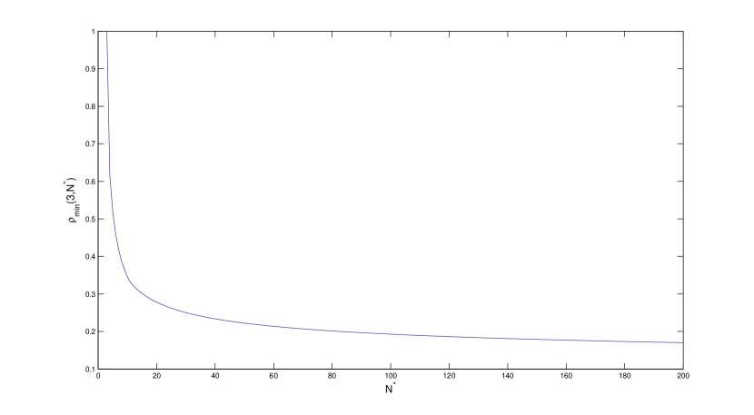
Figure 5: The value of $\rho_{\min}(3,N^{*})$ for $N^{*}=3,4,\cdots,200$.

IX-E Complexity of Lifted Rank-Metric Codes

If we apply Gabidulin codes, a family of MRD codes, the encoding requires $\mathcal{O}((T-M)n^{2}sM)$ operations in $\mathbb{F}$. For decoding, we can apply the algorithm in [20], the complexity of decoding algorithm is given by $\mathcal{O}(D(\mathcal{C}^{(n)})(T-M)n^{2}s^{2})$ operations in $\mathbb{F}$. (Here we consider that one field operation in $GF(q^{m})$ require $\mathcal{O}(m^{2})$ field operations in $\mathbb{F}$.)

X Linear Matrix Codes for LOCs

In general, we require $T>>M$ to achieve $\bar{C}_{\text{CT}}(H,T)$ using lifted rank-metric codes. In this section, we propose another coding scheme that can achieve $\bar{C}_{\text{CT}}$ for all $T\geq M$.

X-A Linear Matrix Codes

Consider $\text{LOC}(H,T)$ with dimension $M\times N$. For any positive real number $s\leq N$, let $\mathbf{G}^{(n)}$ be an $\lfloor ns\rfloor\times nM$ matrix, called the generator matrix. The matrix code generated by $\mathbf{G}^{(n)}$ is

$$\mathcal{G}_{T-M}^{(n)}=\{\mathbf{BG}^{(n)}:\mathbf{B}\in\mathbb{F}^{(T-M)\times\lfloor ns\rfloor}\}.$$

The code for $\text{LOC}(H,T)$ is the lifted matrix code $L(\mathcal{G}_{T-M}^{(n)})$, called lifted linear matrix code. The rate of $L(\mathcal{G}^{(n)})$ is

$$\mathcal{R}^{(n)} =\frac{\log_{2}|\mathbb{F}^{(T-M)\times\lfloor ns\rfloor}|}{nT\log_{2}q}$$

$$=(1-M/T)\lfloor ns\rfloor/n.$$

When $n\rightarrow\infty$, $\mathcal{R}^{(n)}\rightarrow(1-M/T)s$.

Suppose that the transmitted codeword is $L(\mathbf{B}_{0}\mathbf{G}^{(n)})$. The received matrix is given by (31). The decoding equation in (32) now becomes

$$\tilde{\mathbf{Y}}^{(n)}=\mathbf{B}_{0}\mathbf{G}^{(n)}\mathbf{H}^{(n)}.$$ (38)

Since the receiver knows $\mathbf{H}^{(n)}$ and $\mathbf{G}^{(n)}$, the information $\mathbf{B}_{0}$ can be uniquely determined if and only if $\mathbf{G}^{(n)}\mathbf{H}^{(n)}$ is full rank. Thus, the decoding error $P_{e}^{(n)}$ using (38) satisfies

$$P_{e}^{(n)}\leq\Pr\{\operatorname{\text{rk}}(\mathbf{G}^{(n)}H^{(n)})<\lfloor ns\rfloor\}.$$

We can prove the following result in the next subsection.

Theorem 10

Consider linear matrix codes for $\text{LOC}(H,T)$ with dimension $M\times N$, and $(s,\epsilon)$ satisfying $0<s<s+\epsilon<\operatorname{E}[\operatorname{\text{rk}}(H)]$. More than half of the matrices $\mathbf{G}^{(n)}\in\mathbb{F}^{\lfloor ns\rfloor\times nM}$, when used as the generator matrix, give that

$$P_{e}^{(n)}\leq\Pr\{\operatorname{\text{rk}}(\mathbf{G}^{(n)}H^{(n)})<\lfloor ns\rfloor\}<2\left(\frac{q^{-\lfloor n\epsilon\rfloor}}{q-1}+g{(s+\epsilon)}^{n}\right)$$

where $g{(s+\epsilon)}<1$ is defined in (39).

Thus for any $R<\operatorname{E}[\operatorname{\text{rk}}(H)]$, there exists a sequence of lifted linear matrix codes with rate $\mathcal{R}^{(n)}\rightarrow R$ and $P_{e}^{(n)}\rightarrow 0$ as $n\rightarrow\infty$. Moreover, $P_{e}^{(n)}$ decreases exponentially with the increasing of $n$. So lifted linear matrix codes can achieve the rate $(1-T/M)\operatorname{E}[\operatorname{\text{rk}}(H)]$.

X-B Performance of Linear Matrix Codes

Lemma 7 (Chernoff Bound)

Let $\tau_{i}$, $i=1,\cdots,n$, are independent random variables with the same distribution of $\tau\in\{0,1,\cdots,m\}$. For $\alpha<\operatorname{E}[\tau]$,

$$\Pr\left\{\sum_{i}\tau_{i}<n\alpha\right\}\leq g(\alpha)^{n},$$

where

$$g(\alpha) =\operatorname{E}[(A/B)^{(\tau-\alpha)/m}]<1,$$ (39)

$$A =\sum_{r<\alpha}(\alpha-r)p_{\tau}(r),$$

$$B =\sum_{r>\alpha}(r-\alpha)p_{\tau}(r).$$

Proof:

For any $t>0$,

$$\Pr\left\{\sum_{i}\tau_{i}<n\alpha\right\} =\Pr\left\{e^{-t\sum_{i}\tau_{i}}>e^{-tn\alpha}\right\}$$

$$\stackrel{{\scriptstyle\text{(a)}}}{{\leq}}e^{tn\alpha}\operatorname{E}[e^{-t\sum_{i}\tau_{i}}]$$

$$\stackrel{{\scriptstyle\text{(b)}}}{{=}}e^{tn\alpha}\prod_{i}\operatorname{E}[e^{-t\tau_{i}}]$$

$$=\left(e^{t\alpha}\operatorname{E}[e^{-t\tau}]\right)^{n},$$ (40)

where (a) follows from Markov’s inequality and (b) follows from independence.

Now assume $\alpha<\operatorname{E}[\tau]$. Let $f(t)=e^{t\alpha}\operatorname{E}[e^{-t\tau}]$. We know that $f(t)$ is a continuous function for $t\geq 0$ and $f(0)=1$. The first and the second derivatives of $f(t)$ are

$$f^{\prime}(t) =\sum_{r}(\alpha-r)e^{t(\alpha-r)}p_{\tau}(r),\quad\text{and}$$

$$f^{\prime\prime}(t) =\sum_{r}(\alpha-r)^{2}e^{t(\alpha-r)}p_{\tau}(r),$$

respectively. We see that $f^{\prime}(0)=\alpha-\operatorname{E}[\tau]<0$ and $f^{\prime\prime}(t)>0$. Thus, there exists $t_{0}>0$ such that $f^{\prime}(t_{0})=0$ and $f^{\prime}(t)<0$ for $0\leq t<t_{0}$. We give a bound on $t_{0}$ in the following. Let

$$A(t) =\sum_{r<\alpha}(\alpha-r)e^{t(\alpha-r)}p_{\tau}(r),\quad\text{and}$$

$$B(t) =\sum_{r>\alpha}(r-\alpha)e^{t(\alpha-r)}p_{\tau}(r).$$

We see that $A(t)$ and $B(t)$ are monotonically increasing and decreasing, respectively. Since $f^{\prime}(t)=A(t)-B(t)$, we have $A(t_{0})=B(t_{0})$ and $A(0)<B(0)$. Observe that

$$A(t) \leq A(0)e^{t\alpha},$$

$$B(t) \geq B(0)e^{-t(M-\alpha)}.$$

Let $t_{1}$ such that

$$A(0)e^{t_{1}\alpha}=B(0)e^{-t_{1}(M-\alpha)}$$ (41)

We know that $0<t_{1}\leq t_{0}$. Thus, $f(t_{0})\leq f(t_{1})<1$.

By (40),

$$\Pr\left\{\sum_{i}\tau_{i}<n\alpha\right\} \leq\min_{t}f^{n}(t)$$

$$=f^{n}(t_{0})$$

$$\leq f^{n}(t_{1}).$$

Using (41) we have $e^{t_{1}}=(B(0)/A(0))^{1/M}$. The proof is completed by letting $g(\alpha)=f(t_{1})$. ∎

Remark: An alternative to the Chernoff bound is Hoeffding’s inequality, which gives

$$\Pr\left\{\sum_{i}\tau_{i}<n\alpha\right\}\leq\exp\left\{-n\frac{2(\alpha-E[\tau])^{2}}{m^{2}}\right\}.$$

But in our simulation, the error exponent obtained by the Chernoff bound is better than the one obtained using Heoffding’s inequality.

Lemma 8

Suppose that $G^{(n)}$ is an $\lfloor ns\rfloor\times nM$ purely random matrix and independent with $H^{(n)}$. For any $s$ and $\epsilon$ such that $0<s<s+\epsilon<\operatorname{E}[\operatorname{\text{rk}}(H)]$,

$$\Pr\{\operatorname{\text{rk}}(G^{(n)}H^{(n)})<\lfloor ns\rfloor\}<\frac{q^{-\lfloor n\epsilon\rfloor}}{q-1}+g{(s+\epsilon)}^{n},$$

where $g(s+\epsilon)<1$ is defined in (39).

Proof:

Let $F^{(n)}=G^{(n)}H^{(n)}$ and let

$$a_{n}(i)\triangleq\Pr\left\{\operatorname{\text{rk}}(F^{(n)})=\lfloor ns\rfloor|\operatorname{\text{rk}}(H^{(n)})=i\right\}.$$

Let $F_{i}$ be the $i$th row of $F^{(n)}$. Since $G^{(n)}$ contains uniformly independent components, $F_{i}$, $i=1,\cdots,\lfloor ns\rfloor$, are independent and uniformly distributed in the vector space spanned by the row vectors of $H^{(n)}$. For $i\geq\lfloor n(s+\epsilon)\rfloor$,

$$a_{n}(i) \stackrel{{\scriptstyle\text{(a)}}}{{=}}\zeta^{i}_{\lfloor ns\rfloor}$$

$$=\prod_{k=i-\lfloor ns\rfloor+1}^{i}(1-q^{-k})$$

$$>\prod_{k=\lfloor n(s+\epsilon)\rfloor-\lfloor ns\rfloor+1}^{\infty}(1-q^{-k})$$

$$\geq\prod_{k=\lfloor n\epsilon\rfloor+1}^{\infty}(1-q^{-k})$$

$$\geq 1-\sum_{k=\lfloor n\epsilon\rfloor+1}^{\infty}q^{-k}$$

$$=1-q^{-\lfloor n\epsilon\rfloor}/(q-1),$$

where (a) follows from Lemma 11. Moreover, using the Chernoff bound in Lemma 7,

$$\Pr\{\operatorname{\text{rk}}(H^{(n)})<\lfloor n(s+\epsilon)\rfloor\} \leq\Pr\{\operatorname{\text{rk}}(H^{(n)})<n(s+\epsilon)\}$$

$$\leq\left(g(s+\epsilon)\right)^{n},$$

where $g(\cdot)$ is defined in (39) and $g{(s+\epsilon)}<1$. Therefore,

$$\Pr\{\operatorname{\text{rk}}(F^{(n)})=\lfloor ns\rfloor\}$$

$$\geq\sum_{i\geq\lfloor n(s+\epsilon)\rfloor}a_{n}(i)p_{\operatorname{\text{rk}}(H^{(n)})}(i),$$

$$>\left(1-\frac{q^{-\lfloor n\epsilon\rfloor}}{q-1}\right)\Pr\{\operatorname{\text{rk}}(H^{(n)})\geq\lfloor n(s+\epsilon\rfloor\}$$

$$\geq\left(1-\frac{q^{-\lfloor n\epsilon\rfloor}}{q-1}\right)\left(1-g(s+\epsilon)^{-n}\right)$$

$$>1-\frac{q^{-\lfloor n\epsilon\rfloor}}{q-1}-g{(s+\epsilon)}^{n}.$$

The proof is completed. ∎

Lemma 9

Let $0\leq b_{i}\leq 1$, $i=1,\cdots,n$, be a sequence of real numbers. If $\sum_{i=0}^{n}b_{i}/n\leq\epsilon/2$ for some $\epsilon>0$, then there are more than half of the numbers in the sequence with values at most $\epsilon$.

Proof:

Let $\mathcal{A}=\{b_{i}:b_{i}\leq\epsilon\}$. If $|\mathcal{A}|\leq n/2$, then

$$\sum_{i=0}^{n}b_{i} =\sum_{i\in\mathcal{A}}b_{i}+\sum_{i\notin\mathcal{A}}b_{i}$$

$$>\epsilon(n-|\mathcal{A}|)$$

$$\geq n\epsilon/2.$$

We have a contradiction to $\sum_{i=0}^{n}b_{i}/n\leq\epsilon/2$. Thus, $|\mathcal{A}|>n/2$. ∎

Proof:

There are totally $q^{n\lfloor ns\rfloor M}$ $\lfloor ns\rfloor\times nM$ matrices. The average probability of error, when using these matrices uniformly, is upper bounded by

$$\sum_{\mathbf{G}^{(n)}\in\mathbb{F}^{\lfloor ns\rfloor\times nM}}\Pr\{\operatorname{\text{rk}}(\mathbf{G}^{(n)}H^{(n)})<\lfloor ns\rfloor\}q^{-n\lfloor ns\rfloor M}$$

$$=\sum_{\mathbf{G}^{(n)}\in\mathbb{F}^{\lfloor ns\rfloor\times nM}}\Pr\{\operatorname{\text{rk}}(\mathbf{G}^{(n)}H^{(n)})<\lfloor ns\rfloor\}p_{G^{(n)}}(\mathbf{G}^{(n)})$$

$$=\Pr\{\operatorname{\text{rk}}(G^{(n)}H^{(n)})<\lfloor ns\rfloor\}$$

$$\leq\frac{q^{-\lfloor n\epsilon\rfloor}}{q-1}+g{(s+\epsilon)}^{n},$$

where $G^{(n)}$ is a purely random matrix and the last inequality follows from Lemma 8. Thus by Lemma 9, half of these matrices give a probability lower than $2(\frac{q^{-\lfloor n\epsilon\rfloor}}{q-1}+g{(s+\epsilon)}^{n})$. ∎

X-C Complexity of Lifted Linear Matrix Codes

In practice, we can use a pseudorandom generator to generate matrix $\mathbf{G}^{(n)}$, called pseudorandom generator matrix, and share the pseudorandom generator in both the transmitter and the receiver. Discussion of the pseudorandom generator design is out of the scope of this paper. The encoding complexity using a pseudorandom generator matrix is $\mathcal{O}((T-M)Msn^{2})$ and the decoding based on Gaussian elimination requires $\mathcal{O}(n^{3}s^{3}+(T-M)n^{2}s^{2})$ operations in $\mathbb{F}$.

Compared with the lifted Gabidulin Codes, the complexity of decoding a lifted linear Matrix code using Gaussian elimination is higher. To reduce the complexity of encoding and decoding is an important future work to make lifted linear matrix codes practical.

X-D Rateless Coding

Our coding schemes, both the lifted rank-metric codes1 and the lifted linear matrix codes, require only $\operatorname{E}[\operatorname{\text{rk}}(H)]$. Here we show that the lifted linear matrix codes can be realized ratelessly without the knowledge of $\operatorname{E}[\operatorname{\text{rk}}(H)]$ if there exists one-bit feedback from the receiver to the transmitter.

Suppose that we have a sequence of $R\times M$ matrices $\mathbf{G}_{i}$, $i=1,2,\cdots$, called the series of the generator matrices of rateless lifted linear matrix codes, which is known by both the transmitter and the receiver. Here $R$ is a design parameter. Write

$$\mathbf{G}^{(n)}=\begin{bmatrix}\mathbf{G}_{1}&\mathbf{G}_{2}&\cdots&\mathbf{G}_{n}\end{bmatrix}.$$

The transmitter forms its messages into a $(T-M)\times R$ message matrix $\mathbf{B}$, and it keeps on transmitting $L(\mathbf{BG}_{i})$, $i=1,2,\cdots$, until it receives a feedback from the receiver. The $i$th output of the channel is given in (31). After collecting the $n$th output, the receiver checks that if $\mathbf{G}^{(n)}\mathbf{H}^{(n)}$ has rank $R$. If $\mathbf{G}^{(n)}\mathbf{H}^{(n)}$ has rank $R$, the receiver sends a feedback to the transmitter and decodes the message matrix $\mathbf{B}$ by solving the equation $\tilde{\mathbf{Y}}^{n}=\mathbf{B}\mathbf{G}^{(n)}\mathbf{H}^{(n)}$. After received the feedback, the transmitter can transmit another message matrix.

Applying Theorem 10, we can evaluate the performance of the rateless code. The rateless lifted linear matrix codes can achieve the rate $(1-M/T)\operatorname{E}[\operatorname{\text{rk}}(H)]$.

Corollary 5

Consider rateless linear matrix codes for $\text{LOC}(H,T)$ with dimension $M\times N$. There exists a series of generator matrices of rateless lifted linear matrix code $\mathbf{G}_{i}\in\mathbb{F}^{R\times M},i=1,2,\dots$, such that the transmission of one message matrix can be successful decoded with probability at least

$$1-2\left(\frac{q^{-\lfloor n\epsilon\rfloor}}{q-1}+g{(R/n+\epsilon)}^{n}\right)$$

after $n>R/\operatorname{E}[\operatorname{\text{rk}}(H)]$ transmission, where $0<\epsilon<\operatorname{E}[\operatorname{\text{rk}}(H)-R/n$ and $g{(R/n+\epsilon)}<1$ is defined in (39).

XI Concluding Remarks

Linear operator channel is a general channel model that including linear network coding as well as the classical $Z$-channel as special cases. We studied LOCs with general distributions of transformation matrices.

This work showed that the expectation of the rank of the transformation matrix $\operatorname{E}[\operatorname{\text{rk}}(H)]$ is an important parameter of $\text{LOC}(H,T)$. Essentially, this is the best rate that noncoherent transmission can asymptotically achieve when $T$ goes to infinity. We show that both subspace coding and channel training can achieve at least $(1-M/T)\operatorname{E}[\operatorname{\text{rk}}(H)]$.

This work studied subspace coding from an information theoretic point of view. Compared with general subspace coding, constant-dimensional subspace coding can achieve almost the same rate. Given a LOC, we determined the maximum achievable rate of using constant-dimensional subspace coding, as well as the optimal dimension.

We determined the maximum achievable rate of using channel training. The advantage of subspace coding over channel training in terms of rates is not significant for typical channel parameters. So considering channel training for LOCs is sufficient for most scenarios. We proposed two coding approaches for LOCs based on channel training and evaluate their performance.

Many problems about LOCs need further investigation. For small $T$ (e.g., $T\leq M$), we are still lack of good bounds and coding schemes. It is possible to extend this work to LOCs with additive errors and multi-user communication scenarios. Moreover, efficient encoding and decoding algorithms for the coding approaches we proposed are required for practical applications.

Appendix A Counting

Parts of the counting problems here can be found in various sources, e.g., [29, 30] and reference therein. Here we give the self-contained proofs.

Lemma 10

When $0\leq r\leq m$, $|\operatorname{Fr}(\mathbb{F}^{m\times r})|=\chi^{m}_{r}$

Proof:

The lemma is trivial for $r=0$, so we consider $r>0$. We can count the number of full rank matrices in $\mathbb{F}^{m\times r}$ by the columns. For the first column, we can choose all vectors in $\mathbb{F}^{m}$ except the zero vector. Thus we have $q^{m}-1$ choices. Fixed the first column, say $v_{1}$, we want to choose the second column $v_{2}$ in $\mathbb{F}^{m}$ but is linear independent with $v_{1}$. Hence, we have $q^{m}-q$ choices of $v_{2}$. Repeat this process, we can obtain that the number of full rank $m\times r$ matrices is $(q^{m}-1)(q^{m}-q)\cdots(q^{m}-q^{r-1})=\chi^{m}_{r}$. ∎

Recall

$$\zeta^{m}_{r}=\left\{\begin{array}[]{ll}(1-q^{-m})(1-q^{-m+1})\cdots(1-q^{-m+r-1})&r>0\\ 1&r=0\end{array}\right.$$

for $r\leq m$.

Lemma 11

Let $G$ be an $s\times m$ random matrix with uniformly independent components over $\mathbb{F}$. Then for $r\leq m$,

$$p_{\operatorname{\text{rk}}(GH)|\operatorname{\text{rk}}(H)}(s|r)=\zeta^{s}_{r},$$

where $H$ is any $m\times n$ random matrix.

Proof:

Fix an $m\times n$ matrix $\mathbf{H}$ with $\operatorname{\text{rk}}(\mathbf{H})=r$. Let $F=G\mathbf{H}$ and let $g_{i}$ and $f_{i}$ be the $i$th row of $G$ and $F$, respectively. Since $g_{i}$ contains uniformly independent components,

$$\Pr\{{g_{i}}=\mathbf{g}\}=q^{-m}.$$

For $\mathbf{f}$ with $\mathbf{f}^{\top}\in\langle\mathbf{H}^{\top}\rangle$,

$$\Pr\{g_{i}\mathbf{H}=\mathbf{f}\} =q^{-m}|\text{Ker}(\mathbf{H})|$$

$$=q^{-r},$$

where $\text{Ker}(\mathbf{H})=\{\mathbf{g}:\mathbf{gH}=\mathbf{0}\}$ and $|\text{Ker}(\mathbf{H})|=q^{m-\operatorname{\text{rk}}(\mathbf{H})}$. So for $\mathbf{F}$ with $\langle\mathbf{F}^{\top}\rangle\leq\langle\mathbf{H}^{\top}\rangle$,

$$p_{GH|H}(\mathbf{F}|\mathbf{H}) =\Pr\{g_{i}\mathbf{H}=\mathbf{f}_{i},i=1,\cdots,s\}$$

$$=\prod_{i=1}^{s}\Pr\{g_{i}\mathbf{H}=\mathbf{f}_{i}\}$$

$$=q^{-sr}.$$ (42)

Thus,

$$p_{\operatorname{\text{rk}}(GH)|H}(s|\mathbf{H}) =q^{-mr}|\{\mathbf{F}:\langle\mathbf{F}^{\top}\rangle\leq\langle\mathbf{H}^{\top}\rangle,\operatorname{\text{rk}}(\mathbf{F})=s\}|$$

$$=q^{-mr}\chi^{r}_{s}$$

$$=\zeta^{r}_{s},$$

where $|\{\mathbf{F}:\langle\mathbf{F}^{\top}\rangle\leq\langle\mathbf{H}^{\top}\rangle,\operatorname{\text{rk}}(\mathbf{F})=s\}|=\chi^{r}_{s}$ follows from Lemma 10. Last, since $\operatorname{\text{rk}}(H)\rightarrow H\rightarrow\operatorname{\text{rk}}(GH)$ forms a Markov chain,

$$p_{\operatorname{\text{rk}}(GH)|\operatorname{\text{rk}}(H)}(s|r) =\sum_{\mathbf{H}:\operatorname{\text{rk}}(\mathbf{H})=r}p_{\operatorname{\text{rk}}(GH)|H}(s|\mathbf{H})p_{H|\operatorname{\text{rk}}(H)}(\mathbf{H}|r)$$

$$=\zeta^{r}_{s}\sum_{\mathbf{H}:\operatorname{\text{rk}}(\mathbf{H})=r}p_{H|\operatorname{\text{rk}}(H)}(\mathbf{H}|r)$$

$$=\zeta^{r}_{s}.$$

The proof is complete. ∎

Lemma 12

The number of $r$-dimensional subspace in $\mathbb{F}^{m}$ is given by the Gaussian binomials.

Proof:

Define an equivalent relation on $\mathcal{M}(\mathbb{F}^{m\times r})$ by $\mathbf{X}\sim\mathbf{X}^{\prime}$ if $\langle\mathbf{X}\rangle=\langle\mathbf{X}^{\prime}\rangle$. The equivalent class $[\mathbf{X}]$ is the set of all matrices that equivalent to $\mathbf{X}$. We have $[\mathbf{X}]=\{\mathbf{X}\Phi:\Phi\in\mathcal{M}(\mathbb{F}^{r\times r})\}$. Thus $|[\mathbf{X}]|=|\mathcal{M}(\mathbb{F}^{r\times r})|=\chi^{r}_{r}$. Since $\operatorname{Gr}(r,\mathbb{F}^{T})=\mathcal{M}(\mathbb{F}^{m\times r})/\sim$, the quotient set of $\mathcal{M}(\mathbb{F}^{m\times r})$ by $\sim$, we have $|\operatorname{Gr}(r,\mathbb{F}^{T})|=|\mathcal{M}(\mathbb{F}^{m\times r})|/|[\mathbf{X}]|={\chi^{m}_{r}}/{\chi^{r}_{r}}$. ∎

Lemma 13

For $m\geq r^{\prime}$ and $r\geq r^{\prime}$, define a set $S=\{\mathbf{X}\in\mathbb{F}^{m\times r}:\operatorname{\text{rk}}(\mathbf{X})=r^{\prime}\}$. Then

$$|S|=\frac{\chi^{m}_{r^{\prime}}\chi^{r}_{r^{\prime}}}{\chi^{r^{\prime}}_{r^{\prime}}}=\chi^{m,r}_{r^{\prime}}.$$ (43)

Furthermore,

$$\sum_{r^{\prime}}\chi^{m,r}_{r^{\prime}}=q^{mr}.$$ (44)

Proof:

The column vectors of $\mathbf{X}\in S$ span an $r^{\prime}$-dimensional subspace in a $m$-dimensional vector space. Let $\{{V}_{1},{V}_{2},\ldots{V}_{n}\}$ be the set of $r^{\prime}$-dimensional subspace in a $m$-dimensional vector space, where $n=\left({}^{m}_{r^{\prime}}\right)_{q}$. Let $S_{{V}_{i}}=\{\mathbf{X}\in\mathbb{F}^{m\times r}:\langle\mathbf{X}\rangle={V}_{i}\}$ and the set $\{S_{{V}_{i}}\}$ is a partition of $S$. By $|\{S_{{V}_{i}}\}|=\chi^{r}_{r^{\prime}}$. Therefore,

$$|S|=n|S_{{V}_{i}}|=\left({}^{m}_{r^{\prime}}\right)_{q}\chi^{r}_{r^{\prime}}=\chi^{m,r}_{r^{\prime}}.$$ (45)

The equality in (44) follows because both sides are the number of $m\times r$ matrices. ∎

Lemma 14

Let $V\leq\mathbb{F}^{m}$ be a $s$-dimensional subspace. Then, the number of subspace $U$ with $V\leq U$ and $\dim(U)=r$ is

$$\left({}^{m-s}_{r-s}\right)_{q}=\left({}^{m}_{r}\right)_{q}\frac{\chi^{r}_{s}}{\chi^{m}_{s}}.$$ (46)

Proof:

Let $U$ be a subspace with $V\leq U$ and $\dim(U)=r$. Then we can write $U=V+U^{\prime}$ where $U^{\prime}$ is a $\dim(U^{\prime})=r-s$ and $V\cap U^{\prime}=\{0\}$. Given $U$, such $U^{\prime}$ is unique. The number of $U^{\prime}$ is the number of $(r-s)$-dimensional subspace in an $(m-s)$-dimensional space, i.e., $\left({}^{m-s}_{r-s}\right)_{q}$. The equality in (46) is the direct result of the definitions. ∎

Appendix B Useful Results

Lemma 15

For $r\leq m$, $-\log_{2}\zeta^{m}_{r}<1.8$.

Proof:

Define

$$\Xi_{q}(s)=\prod_{i=s}^{\infty}(1-q^{-i}).$$ (47)

So $\zeta^{m}_{r}>\Xi_{q}(m-r+1)$. We know $\Xi_{q}(s+1)>\Xi_{q}(s)>\Xi_{q-1}(s)\geq\Xi_{2}(1)$, where $\Xi_{2}(1)$ is a mathematics constant with approximate value $0.28879$ [30]. Thus $-\log_{2}\zeta^{m}_{r}\leq-\log_{2}\Xi_{2}(1)<-\log_{2}0.2887<1.8$. ∎

Lemma 16

$\lim_{T\rightarrow\infty}\frac{\log_{2}\chi^{T}_{r}}{T\log_{2}q}=r$.

Proof:

$$\lim_{T\rightarrow\infty}\frac{\log_{2}\chi^{T}_{r}}{T\log_{2}q} =\lim_{T\rightarrow\infty}\frac{\log_{2}\zeta^{T}_{r}q^{Tr}}{T\log_{2}q}$$

$$=\lim_{T\rightarrow\infty}\frac{\log_{2}\zeta^{T}_{r}}{T\log_{2}q}+\lim_{T\rightarrow\infty}\frac{\log_{2}q^{Tr}}{T\log_{2}q}$$

$$=0+r.$$

∎

Lemma 17

$|\operatorname{Pj}(\mathbb{F}^{m})|<q^{m^{2}/2+\log_{q}m+c}$, where $c<1.8$ is a constant.

Proof:

Refer to the proof of Lemma 15. We have

$$|\operatorname{Pj}(\mathbb{F}^{m})| =\sum_{r\leq m}\begin{pmatrix}m\\ r\end{pmatrix}_{q}$$

$$=\sum_{r\leq m}q^{(m-r)r}\frac{\zeta^{m}_{r}}{\zeta^{r}_{r}}$$

$$<\sum_{r\leq m}q^{(m-r)r}\frac{1}{\Xi_{q}(1)}$$

$$<\frac{m}{\Xi_{q}(1)}q^{m^{2}/2}$$

$$=q^{m^{2}/2+\log_{q}(m/\Xi_{q}(1))}$$

$$<q^{m^{2}/2+\log_{q}m+\log_{2}(1/\Xi_{2}(1))}.$$

Let $c=\log_{2}(1/\Xi_{2}(1))$. By $\Xi_{2}(1)\approx 0.28879$, we obtain $c<1.8$. ∎

Lemma 18

For $V\leq U\leq\mathbb{F}^{T}$ and $V^{\prime}\leq U^{\prime}\leq\mathbb{F}^{T}$ with $\dim(U)=\dim(U^{\prime})$ and $\dim(V)=\dim(V^{\prime})$, we can find $\Phi\in\operatorname{Fr}(\mathbb{F}^{T\times T})$ such that $\Phi U=U^{\prime}$ and $\Phi V=V^{\prime}$.

Proof:

Find a basis $\{\mathbf{b}_{i}:i=1,\cdots,T\}$ of $\mathbb{F}^{T}$ such that $\{\mathbf{b}_{i}:i=1,\cdots,r\}$ is a basis of $U$ and $\{\mathbf{b}_{i}:i=1,\cdots,s\}$ is a basis of $V$. We can do this by first finding a basis of $V$, extending the basis to a basis of $U$ and further extending to a basis of $\mathbb{F}^{T}$. Similarly, find a basis $\{\mathbf{b}^{\prime}_{i}:i=1,\cdots,T\}$ of $\mathbb{F}^{T}$ such that $\{\mathbf{b}^{\prime}_{i}:i=1,\cdots,r\}$ is a basis of $U$ and $\{\mathbf{b}^{\prime}_{i}:i=1,\cdots,s\}$ is a basis of $V$. Consider the linear system of equations

$$\Phi\mathbf{b}_{i}=\mathbf{b}_{i}^{\prime},\quad i=1,\cdots,T.$$

We know there exists unique $\Phi\in\operatorname{Fr}(\mathbb{F}^{T\times T})$ satisfying this linear system and $\Phi V=V^{\prime}$ and $\Phi U=U^{\prime}$. ∎

Lemma 19

For $\mathbf{X},\mathbf{X}^{\prime}\in\mathbb{F}^{T\times M}$, $\langle\mathbf{X}^{\top}\rangle=\langle\mathbf{X}^{\prime\top}\rangle$ if and only if there exists $\Phi\in\operatorname{Fr}(\mathbb{F}^{T\times T})$ such that $\mathbf{X}^{\prime}=\Phi\mathbf{X}$.

Proof:

Let $r=\operatorname{\text{rk}}(\mathbf{X})$. First, show a) $\Rightarrow$ c). Fix one full-rank decomposition $\mathbf{X}=\mathbf{B}\mathbf{D}$. Since $\langle\mathbf{D}^{\top}\rangle=\langle\mathbf{X}^{\top}\rangle=\langle\mathbf{X}^{\prime\top}\rangle$, we can find a decomposition $\mathbf{X}^{\prime}=\mathbf{B}^{\prime}\mathbf{D}$ using the same procedure we described by first fixing $\mathbf{D}$. Second, show c) $\Rightarrow$ b). With the decomposition in c), we can find $\Phi\in\operatorname{Fr}(\mathbb{F}^{T\times T})$ such that $\Phi\mathbf{B}=\mathbf{B}^{\prime}$. Extend $\mathbf{B}$ and $\mathbf{B}^{\prime}$ to $T\times T$ matrices $[\mathbf{B}\ \mathbf{B}_{0}]$ and $[\mathbf{B}^{\prime}\ \mathbf{B}_{0}^{\prime}]$. Then, $\Phi=[\mathbf{B}^{\prime}\ \mathbf{B}_{0}^{\prime}][\mathbf{B}\ \mathbf{B}_{0}]^{-1}$ is one such matrix we want since $\Phi[\mathbf{B}\ \mathbf{B}_{0}]=[\mathbf{B}^{\prime}\ \mathbf{B}_{0}^{\prime}]$. Last, we have b) $\Rightarrow$ a). ∎

Lemma 20

For $U\leq\mathbb{F}^{t}$ with $\dim(U)=r\leq m$, let

$$A(m,U)=\{\mathbf{X}\in\mathbb{F}^{t\times m}:\langle\mathbf{X}\rangle=U\}.$$

Then,

$$|A(m,U)|=\chi^{m}_{r},$$

and for $\Phi\in\operatorname{Fr}(\mathbb{F}^{t\times t})$

$$A(m,\Phi U)=\Phi A(m,U).$$

Proof:

Find a $t\times r$ matrix $\mathbf{B}$ with $\langle\mathbf{B}\rangle=U$. Then, we have

$$A(m,U)=\{\mathbf{BD}:\mathbf{D}\in\operatorname{Fr}(\mathbb{F}^{r\times m})\}=\mathbf{B}\operatorname{Fr}(\mathbb{F}^{r\times m}).$$

Thus, $|A(m,U)|=|\operatorname{Fr}(\mathbb{F}^{r\times m})|=\chi^{m}_{r}$. For $\Phi\in\operatorname{Fr}(\mathbb{F}^{t\times t})$, $\langle\Phi\mathbf{B}\rangle=\Phi U$. So $A(m,\Phi U)=\Phi\mathbf{B}\operatorname{Fr}(\mathbb{F}^{r\times M})=\Phi A(m,U)$. ∎

References

- [1] R. Ahlswede, N. Cai, S.-Y. R. Li, and R. W. Yeung, “Network information flow,” IEEE Trans. Inform. Theory, vol. 46, no. 4, pp. 1204–1216, Jul. 2000.
- [2] S.-Y. R. Li, R. W. Yeung, and N. Cai, “Linear network coding,” IEEE Trans. Inform. Theory, vol. 49, no. 2, pp. 371–381, Feb. 2003.
- [3] R. Koetter and M. Medard, “An algebraic approach to network coding,” IEEE/ACM Trans. Networking, vol. 11, no. 5, pp. 782–795, Oct. 2003.
- [4] S. Jaggi, P. Sanders, P. A. Chou, M. Effros, S. Egner, K. Jain, and L. Tolhuizen, “Polynomial time algorithms for multicast network code construction,” IEEE Trans. Inform. Theory, vol. 51, no. 6, pp. 1973 – 1982, Jun. 2005.
- [5] S. Avestimehr, S. N. Diggavi, and N. D. C. Tse, “Wireless network information flow,” in Proc. Allerton Conference 2007, 2007.
- [6] ——, “A deterministic approach to wireless relay networks,” in Proc. Allerton Conference 2007, 2007.
- [7] J. Ebrahimi and C. Fragouli, “Combinatorial algorithms for wireless information flow,” arXiv:0909.4808.
- [8] ——, “Multicasting algorithms for deterministic networks,” in Proc. ITW 2010, 2010.
- [9] T. Ho, M. Medard, R. Koetter, D. R, Karger, M. Effros, J. Shi, and B. Leong, “A random linear network coding approach to multicast,” IEEE Trans. Inform. Theory, vol. 52, no. 10, pp. 4413–4430, Oct. 2006.
- [10] C.Gkantsidis and P.R.Rodriguez, “Network coding for large scale content distribution,” in Proc. INFOCOM, 2005.
- [11] A. G. Dimakis, P. B. Godfrey, M. J. Wainwright, and K. Ramchandran, “Network coding for distributed storage systems,” in Proc. INFOCOM 2007, 2007. [Online]. Available: arXiv:cs/0702015v1
- [12] C. Fragouli, J. Widmer, and J.-Y. L. Boudec, “Efficient broadcasting using network coding,” IEEE/ACM Transactions on Networking, vol. 16, no. 2, 2008.
- [13] M. Xiao and M. Skoglund, “Design of network codes for multiple-user multiple-relay wireless networks,” in Proc. IEEE ISIT’09, Jul. 2009.
- [14] A. Montanari and R. Urbanke, “Coding for network coding,” Nov. 2007, preprint. [Online]. Available: http://arxiv.org/abs/0711.3935
- [15] D. Silva, F. R. Kschischang, and R. Koetter, “Communication over finite-field matrix channels,” Jul. 2009. [Online]. Available: http://arxiv.org/abs/0807.1372
- [16] S. Chachulski, M. Jennings, S. Katti, and D. Katabi, “Trading structure for randomness in wireless opportunistic routing,” in Proc. ACM SIGCOMM, 2007.
- [17] S. Katti, D. Katabi, H. Balakrishnan, and M. Medard, “Symbol-level network coding for wireless mesh networks,” in Proc. ACM SIGCOMM, 2008.
- [18] H. Balli, X. Yan, and Z. Zhang, “Error correction capability of random network error correction codes,” in Proc. IEEE ISIT’07, Jun. 2007.
- [19] R. Koetter and F. R. Kschischang, “Coding for errors and erasures in random network coding,” IEEE Trans. Inform. Theory, vol. 54, no. 8, pp. 3579–3591, Aug. 2008.
- [20] D. Silva, F. Kschischang, and R. Koetter, “A rank-metric approach to error control in random network coding,” IEEE Trans. Inform. Theory, vol. 54, no. 9, pp. 3951–3967, Sept. 2008.
- [21] E. M. Gabidulin, “Theory of codes with maximum rank distance,” Probl. Inform. Transm, vol. 21, no. 1, pp. 1–12, 1985.
- [22] M. J. Siavoshani, C. Fragouli, and S. Diggavi, “Noncoherent multisource network coding,” in Proc. IEEE ISIT’08, Jul. 2008.
- [23] M. Jafari, S. Mohajer, C. Fragouli, and S. Diggavi, “On the capacity of non-coherent network coding,” in Proc. IEEE ISIT’09, Jul. 2009.
- [24] R. G. Gallager, Information Theory and Reliable Communication. John Wiley and Sons, Inc, 1968.
- [25] R. W. Yeung, Information Theory and Network Coding. Springer, 2008.
- [26] R. Koetter and F. R. Kschischang, “Coding for errors and erasures in random network coding,” IEEE Trans. Inform. Theory, vol. 54, no. 8, pp. 3579–3591, Aug. 2008.
- [27] R. W. Nóbrega and B. F. Uchôa-Filho, “Multishot codes for network coding: bounds and a multilevel construction,” in Proc. IEEE ISIT’09, Jul. 2009.
- [28] ——, “Multishot codes for network coding using rank-metric codes,” 2010, submitted to ISIT’10.
- [29] “Wikipedia,” online, http://en.wikipedia.org.
- [30] C. Cooper, “On the distribution of rank of a random matrix over a finite field,” Random Struct. Algorithms, vol. 17, no. 3-4, pp. 197–212, 2000.