Extending canonical Monte Carlo methods II

Abstract

Previously, we have presented a methodology to extend canonical Monte Carlo methods inspired on a suitable extension of the canonical fluctuation relation $C=\beta^{2}\left\langle\delta E^{2}\right\rangle$ compatible with negative heat capacities $C<0$. Now, we improve this methodology by introducing a better treatment of finite size effects affecting the precision of a direct determination of the microcanonical caloric curve $\beta\left(E\right)=\partial S\left(E\right)/\partial E$, as well as a better implementation of MC schemes. We shall show that despite the modifications considered, the extended canonical MC methods possibility an impressive overcome of the so-called super-critical slowing down observed close to the region of a temperature driven first-order phase transition. In this case, the dependence of the decorrelation time $\tau$ with the system size $N$ is reduced from an exponential growth to a weak power-law behavior $\tau(N)\propto N^{\alpha}$, which is shown in the particular case of the 2D seven-state Potts model where the exponent $\alpha=0.14-0.18$.

1 Introduction

In a previous paper [1], we have proposed a methodology that enables Monte Carlo (MC) methods based on the Gibbs canonical ensemble:

$$dp_{c}\left(E\left|\beta_{B}\right.\right)=\frac{1}{Z\left(\beta_{B}\right)}\exp\left(-\beta_{B}E\right)\Omega\left(E\right)dE$$ (1)

to account for the existence of an anomalous region with negative heat capacities $C<0$ [2, 3, 4, 5, 6, 7] and to overcome the so-called supercritical slowing down observed near of first-order phase transition [8]. This development is inspired on the consideration of a recently obtained fluctuation relation [9, 10, 11]:

$$C=\beta^{2}\left\langle\delta E^{2}\right\rangle+C\left\langle\delta\beta_{\omega}\delta E\right\rangle,$$ (2)

which appears as a suitable extension of the known canonical identity $C=\beta^{2}\left\langle\delta E^{2}\right\rangle$ involving the heat capacity $C$ and the energy fluctuations $\left\langle\delta E^{2}\right\rangle$. This last expression accounts for the realistic perturbation provoked on the internal state of a certain environment as a consequence of the underlying thermodynamic interaction with the system under study, which is characterized here in terms of the correlation function $\left\langle\delta\beta_{\omega}\delta E\right\rangle$ between the system internal energy $E$ and the environment inverse temperature $\beta_{\omega}$. While the canonical ensemble (1) dismisses the existence of this feedback effect (due to the constancy of the inverse temperature $\beta_{B}$ associated with this ensemble) and it is only compatible with positive heat capacities, the general case possibilities to access anomalous macrostates with negative heat capacities $C<0$ as long as the condition $\left\langle\delta\beta_{\omega}\delta E\right\rangle>1$ is obeyed.

The incidence of non-vanishing correlated fluctuations $\left\langle\delta\beta_{\omega}\delta E\right\rangle$ can be easily implemented in MC simulations. Roughly speaking, the extension of canonical MC methods is achieved by replacing the canonical inverse temperature $\beta_{B}$ with a variable inverse temperature $\beta_{\omega}\left(E\right)$. The resulting framework constitutes a suitable extension of the Gerling and Hüller methodology on the basis of the so-called dynamic ensemble [12], where the microcanonical curve $\beta\left(E\right)=\partial S\left(E\right)/\partial E$ and the heat capacity $C\left(E\right)$ can be estimated in terms of the energy and temperature expectation values $\left\langle E\right\rangle$ and $\left\langle\beta_{\omega}\right\rangle$ as well as their fluctuating behavior described by Eq.(2). This method successfully reduces the exponential divergence of decorrelation time $\tau\propto\exp\left(\lambda N\right)$ with the increase of the system size $N$ of canonical MC methods to a weak power-law divergence $\tau\propto N^{\alpha}$, with a typical exponent $\alpha\simeq 0$.$2$ for the case of $2D$ ten-state Potts model [1]. By combining this type of argument with cluster algorithms, one obtains very efficient MC schemes that constitute attractive alternatives of the known multicanonical method and its variants [8]. In this work, we shall improve the present methodology to consider the existence of finite size effects that reduces the precision of a direct determination of the microcanonical caloric curve $\beta\left(E\right)=\partial S\left(E\right)/\partial E$, as well as a better implementation of MC schemes.

2 Methodology

2.1 Overview

The simplest way to implement the existence of non-vanishing correlations $\left\langle\delta\beta_{\omega}\delta E\right\rangle$ corresponds to a linear coupling of the environment inverse temperature $\beta_{\omega}$ with the thermal fluctuations of the system energy:

$$\beta_{\omega}\left(E\right)=\beta_{e}+\lambda\delta E/N,$$ (3)

where $\lambda$ is a coupling constant that appears here as an additional control parameter. While the case with $\lambda=0$ corresponds to the canonical ensemble (1), where $\beta_{\omega}=const$, in general, the constancy of the inverse temperature $\beta_{e}$ can be only ensured in the average sense, $\beta_{e}=\left\langle\beta_{\omega}\right\rangle$. Eq.(3) can be substituted into Eq.(2) to obtain the following results:

$$\left(\Delta E\right)^{2}=\frac{N}{\beta^{2}N/C+\lambda},~{}\left(\Delta\beta_{\omega}\right)^{2}=\frac{1}{N}\frac{\lambda^{2}}{\beta^{2}N/C+\lambda},$$ (4)

where $\Delta x\equiv\sqrt{\left\langle\delta x^{2}\right\rangle}$ denotes the thermal dispersion of a given quantity $x$. Since $\Delta\beta_{\omega}$ and $\Delta E$ should be nonnegative, one arrives at the following stability condition:

$$\beta^{2}N/C+\lambda>0.$$ (5)

For $\lambda=0$, one derives the ordinary constraint $C>0$ that emphasizes the unstable character of macrostates with negative heat capacities $C<0$ within the canonical description. However, these anomalous macrostates can be observed in a stable way in a general situation with $\lambda\not=0$ when this control parameter satisfies Eq.(5). By assuming an extensive character of the heat capacity $C\sim N$ in short-range interacting systems, the energy dispersion $\Delta E$ grows with the increase of the system size $N$ as $\Delta E\sim\sqrt{N}$, so that, the dispersion of the energy per particle $\varepsilon=E/N$ behaves as $\Delta\varepsilon\sim 1/\sqrt{N}$. Since $\delta\beta_{\omega}\equiv\lambda\delta E/N$ in the case of the ansatz (3), the dispersion of the inverse temperature also behaves as $\Delta\beta_{\omega}\sim 1/\sqrt{N}$. Thus, the present equilibrium situation constitutes a physical scenario that ensures the stability of macrostates with negative heat capacities $C<0$ with the incidence of small thermal fluctuations.

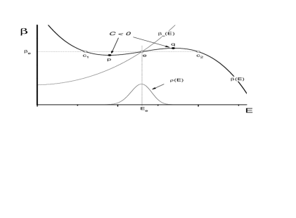
Figure 1: Schematic representation of the typical microcanonical caloric curve $\beta\left(E\right)=\partial S\left(E\right)/\partial E$ associated with a finite short-range interacting system undergoing a first-order phase transition, as well as the energy distribution function $\rho\left(E\right)$ resulting from the thermal coupling of this system with a certain environment with inverse temperature $\beta_{\omega}\left(E\right)$. For further explanations, see the text.

This type of equilibrium situation is schematically represented in FIG.1. Here, it is shown the typical microcanonical caloric curve $\beta\left(E\right)=\partial S\left(E\right)/\partial E$ corresponding to a finite short-range interacting system that undergoes a first-order phase transition, as well as the energy distribution function $\rho\left(E\right)$ associated with the thermal coupling of this system with an environment with inverse temperature $\beta_{\omega}\left(E\right)$. The intersection points $E_{e}$ derived from the condition of thermal equilibrium:

$$\beta\left(E_{e}\right)=\beta_{\omega}\left(E_{e}\right)$$ (6)

determine the position of maxima and minima of the distribution function $\rho\left(E\right)$. Note that the linear ansatz (3) can be considered as the first-order approximation of the power expansion of a general dependence $\beta_{\omega}(E)$:

$$\beta_{\omega}(E)=\beta_{e}+\sum^{\infty}_{n=1}a_{n}(E-E_{e})^{n},$$ (7)

where $a_{1}=\partial\beta_{\omega}(E_{e})/\partial E\equiv\lambda/N$. While in the canonical ensemble there could exist three intersections points ($e$, $c_{1}$ and $c_{2}$) because of the constancy of the inverse temperature, it is possible to ensure the existence of only one intersection point $E_{e}$ by appropriately choosing the inverse temperature dependence $\beta_{\omega}\left(E\right)$. If the system size $N$ is sufficiently large, the energy distribution function $\rho\left(E\right)$ adopts a bell shape, which is approximately described with the Gaussian distribution:

$$\rho\left(E\right)\simeq A\exp\left[-\frac{1}{2\sigma_{E}^{2}}\left(E-E_{e}\right)^{2}\right],$$ (8)

where $\sigma_{E}=\Delta E$. The expectation values $\left\langle E\right\rangle$ and $\left\langle\beta_{\omega}\right\rangle$ provide a direct estimation of the energy $E_{e}$ and inverse temperature $\beta_{e}=\beta\left(E_{e}\right)$ at the intersection point illustrated in FIG.1:

$$E_{e}=\left\langle E\right\rangle,~{}\beta_{e}=\left\langle\beta_{\omega}\right\rangle.$$ (9)

The procedure previously described is equivalent to the one employed by Gerling and Hüller in the framework of the dynamical ensemble [12]:

$$\omega_{D}\left(E\right)=A\left(E_{T}-E\right)^{B},$$ (10)

which accounts for the thermal coupling of the system with a bath exhibiting a constant heat capacity, e.g., an ideal gas, whose inverse temperature obeys the following dependence on the system energy $E$:

$$\beta_{\omega}\left(E\right)=B/\left(E_{T}-E\right).$$ (11)

Our proposal considers some improvements to the Gerling and Huller’s methodology. In fact, the energy dependence (11) is less convenient for calculations than the linear ansatz (3), which is a feature particularly useful to perform the analysis of finite size effects (see subsection 2.2 below). Moreover, one can also obtain the value of the heat capacity $C\left(E\right)$, or more exactly, the so-called curvature curve $\kappa\left(E\right)$:

$$\kappa\left(E\right)=\beta^{2}N/C\equiv-N\frac{\partial^{2}S\left(E\right)}{\partial E^{2}}$$ (12)

at the intersection point $E_{e}$, $\kappa_{e}=\kappa\left(E_{e}\right)$, through the energy dispersion $\Delta E$ in analogous way of MC calculation by using the canonical ensemble (1):

$$\kappa_{e}=\frac{1-\lambda\left(\Delta E\right)^{2}/N}{\left(\Delta E\right)^{2}/N}.$$ (13)

This last equation was obtained from Eq.(12) by rewriting the first relation of Eq.(4).

Since the energy and the inverse temperature dispersions in Eq.(4) are controlled by the coupling constant $\lambda$, it is desirable to reduce them as low as possible. One can verify that the energy dispersion $\Delta E$ decreases with the increase of the coupling constant $\lambda$. However, the value of this parameter should not be excessively large. Its increment leads to the increase of the inverse temperature dispersion $\Delta\beta_{\omega}$, which affects the precision of the inverse temperature $\beta_{e}$ of the system indirectly derived from the expectation value $\left\langle\beta_{\omega}\right\rangle$. A thermodynamic criterion to provide an optimal value for the coupling constant $\lambda$ can be obtained by minimizing the total dispersion $\Delta_{T}^{2}$:

$$\Delta_{T}^{2}=\frac{\left(\Delta E\right)^{2}}{N}+N\left(\Delta\beta_{\omega}\right)^{2}=\frac{1+\lambda^{2}}{\lambda+\kappa_{e}},$$ (14)

which talks about the precision in the determination of the intersection point $\left(E_{e},\beta_{e}\right)$. This analysis leads to the following result:

$$\lambda_{\Delta}=\lambda_{\Delta}\left(\kappa_{e}\right)=\sqrt{1+\kappa_{e}^{2}}-\kappa_{e},~{}\min\Delta_{T}^{2}=2\lambda_{\Delta}$$ (15)

2.2 Finite size effects

The energy distribution function corresponding to the thermal coupling of the system with an environment can be expressed by the following equation:

$$\rho\left(E\right)dE=\omega\left(E\right)\Omega\left(E\right)dE.$$ (16)

Here, $\omega\left(E\right)$ is a probabilistic weight that characterizes such a thermodynamic influence, which is related to the environment inverse temperature $\beta_{\omega}\left(E\right)$ as follows:

$$\beta_{\omega}\left(E\right)=-\frac{\partial\log\omega\left(E\right)}{\partial E}.$$ (17)

A direct integration allows us to verify that the probabilistic weight associated with the linear ansatz (3) is simply the Gaussian ensemble [15]:

$$\omega_{G}\left(E\right)=\frac{1}{Z_{\lambda}\left(\beta_{e}\right)}\exp\left[-\beta_{e}E-\frac{1}{2N}\lambda\left(E-E_{e}\right)^{2}\right]$$ (18)

introduced by Hetherington [16], which approaches in the limit $\lambda\rightarrow+\infty$ to the microcanonical ensemble:

$$\omega_{M}=\frac{1}{\Omega}\delta\left(E-E_{e}\right).$$ (19)

As already explained, the estimation of the microcanonical caloric curve $\beta\left(E\right)$, as well as the fluctuation relation (2), are based on the consideration of a Gaussian shape for the energy distribution function $\rho\left(E\right)$. Such an approximation naturally arises as the asymptotic distribution as long as the system size $N$ be sufficiently large. If the system size $N$ is not so large, small deviations from the Gaussian profile (8) are naturally expected. Fortunately, the particular mathematical form of the Gaussian ensemble (18) possibilities to consider some simple corrections formulae to deal with the existence of these finite size effects and to improve the precision of the present methodology.

Let us denote the energy distribution function in terms of the energy per particle $\varepsilon=E/N$ as follows:

$$\rho\left(\varepsilon\right)=\frac{1}{Z_{\lambda}}\exp\left[-N\phi\left(\varepsilon\right)\right],$$ (20)

where the function $\phi\left(\varepsilon\right)\equiv\beta_{e}\varepsilon+\frac{1}{2}\lambda\left(\varepsilon-\varepsilon_{e}\right)^{2}-s\left(\varepsilon\right)$, with $s\left(\varepsilon\right)$ being the entropy per particle, and $\beta_{e}$:

$$\beta_{e}=\frac{\partial s\left(\varepsilon_{e}\right)}{\partial\varepsilon},$$ (21)

the system inverse temperature at the stationary point $\varepsilon_{e}$. Let us now develop a power-expansion:

$$\phi\left(\varepsilon_{e}+x\right)=\phi\left(\varepsilon_{e}\right)+\frac{1}{2}\left(\lambda+\kappa_{e}\right)x^{2}+\sum_{n=3}^{\infty}a_{n}x^{n},$$ (22)

with $\kappa_{e}=-\partial^{2}s\left(\varepsilon_{e}\right)/\partial\varepsilon^{2}$ being the curvature. The Gaussian approximation is developed by dismissing those terms with $n>2$. Here, the energy deviation $x$ obeys a Gaussian distribution:

$$\rho^{\left(0\right)}\left(x\right)dx\simeq\frac{1}{\sqrt{2\pi}\sigma}\exp\left(-\frac{x^{2}}{2\sigma^{2}}\right)dx$$ (23)

with standard deviation $\sigma$:

$$\sigma^{2}=\frac{1}{N\left(\lambda+\kappa_{e}\right)},$$ (24)

and the partition function $Z_{\lambda}$ can be approximated as:

$$Z_{\lambda}=e^{-N\phi(\varepsilon_{e})}\sqrt{2\pi}\sigma.$$ (25)

Note that Eq.(24) is fully equivalent to Eq.(13) since the standard deviation $\sigma\equiv\Delta E/N$. Eq.(25) can be rewritten as follows:

$$P_{\lambda}\simeq\beta_{e}E_{e}-S\left(E_{e}\right)+\frac{1}{2}\log\left(2\pi\sigma^{2}\right),$$ (26)

where $P_{\lambda}=-\log Z_{\lambda}$ can be referred to as the Plank thermodynamic potential corresponding to the Gaussian ensemble (18). By performing the thermodynamic limit $N\rightarrow\infty$, this thermodynamic function can be related to the known Legendre transformation with the microcanonical entropy:

$$p_{\lambda}=\lim_{N\rightarrow\infty}\frac{P_{\lambda}}{N}=\beta_{e}\varepsilon_{e}-s\left(\varepsilon_{e}\right).$$ (27)

Clearly, the Gaussian ensemble (18) provides a suitable extension of the Gibbs canonical ensemble (1) that is able to deal with the existence of macrostates with negative heat capacities $C<0$. In fact, it is a particular example of the so-called generalized canonical ensembles that preserve some of its more relevant features [11, 17, 18].

The first correction of the Gaussian approximation (23) is obtained by dismissing terms with $n>3$ in the power expansion (22):

$$N\phi\left(x\right)=N\phi_{0}+\frac{1}{2\sigma^{2}}x^{2}+\xi x^{3}+O\left(x^{4}\right),$$ (28)

where:

$$\xi=-\frac{1}{6}N\frac{\partial^{3}s\left(\varepsilon_{e}\right)}{\partial\varepsilon^{3}}.$$ (29)

It is convenient to introduce the dimensionless variable $\theta=x/\sigma$. By considering the size dependencies $\xi\sim N$ and $\sigma\sim 1/\sqrt{N}$, it is possible to verify that the cubic term $\xi x^{3}\equiv\xi\sigma^{3}\theta^{3}$ decreases as $1/\sqrt{N}$ with the increase of the system size $N$. Thus, one arrives at the distribution function:

$$\rho^{\left(1\right)}\left(\theta\right)d\theta\simeq\frac{1}{\sqrt{2\pi}}e^{-\frac{1}{2}\theta^{2}}\left(1-\xi\sigma^{3}\theta^{3}\right)d\theta.$$ (30)

This last result leads to the following expectation values:

$$\left\langle\theta\right\rangle=-3\xi\sigma^{3},~{}\left\langle\theta^{2}\right\rangle=1,~{}\left\langle\theta^{3}\right\rangle=-15\xi\sigma^{3},$$ (31)

which allow to express the expectation value of the energy deviation $\left\langle x\right\rangle$ as well as its second and third order dispersions, $\left\langle\delta x^{2}\right\rangle$ and $\left\langle\delta x^{3}\right\rangle$, as follows:

$$\left\langle x\right\rangle = -3\xi\sigma^{4}+O\left(\frac{1}{N^{2}}\right),\left\langle\delta x^{2}\right\rangle=\sigma^{2}+O\left(\frac{1}{N^{2}}\right),$$ (32)

$$~{}\left\langle\delta x^{3}\right\rangle = -6\xi\sigma^{6}+O\left(\frac{1}{N^{3}}\right).$$ (33)

The previous results can be combined with the linear ansatz (3) to obtain the following first-order correction of Eq.(9):

$$E_{e} =\left\langle E\right\rangle-\frac{1}{2\left\langle\delta E^{2}\right\rangle}\left\langle\delta E^{3}\right\rangle,$$ (34)

$$\beta_{e} =\left\langle\beta_{\omega}\right\rangle-\lambda\frac{1}{2N\left\langle\delta E^{2}\right\rangle}\left\langle\delta E^{3}\right\rangle.$$ (35)

The second-order correction of the Gaussian constributions is carried out by dismissing terms with $n>4$ in power expansion (22):

$$N\phi\left(x\right)=\frac{1}{2\sigma^{2}}x^{2}+\xi x^{3}+\xi_{2}x^{4}+O\left(x^{5}\right),$$ (36)

where:

$$\xi_{2}=-\frac{1}{24}N\frac{\partial^{4}s\left(\varepsilon_{e}\right)}{\partial\varepsilon^{4}}.$$ (37)

These terms lead to the following correction of the distribution function:

$$\rho^{\left(2\right)}\left(\theta\right)d\theta\simeq\frac{e^{-\frac{1}{2}\theta^{2}}}{A\sqrt{2\pi}}\left(1-\xi\sigma^{3}\theta^{3}-\xi_{2}\sigma^{4}\theta^{4}+\frac{1}{2}\xi^{2}\sigma^{6}\theta^{6}\right)d\theta.$$ (38)

whose third and fourth terms account for finite size effects of order $O\left(1/N\right)$. By denoting the auxiliary constants $C_{1}$ and $C_{2}$ as follows:

$$C_{1}=\xi\sigma^{3},~{}C_{2}=\xi_{2}\sigma^{4},$$ (39)

direct calculations allow to obtain the normalization constant $A$:

$$A=1-3C_{2}+\frac{15}{2}C_{1}^{2},$$ (40)

as well as the following expectation values:

$$\left\langle\theta\right\rangle =-3C_{1},~{}\left\langle\theta^{2}\right\rangle=1-12C_{2}+45C_{1}^{2},$$ (41)

$$\left\langle\theta^{3}\right\rangle =-15C_{1},~{}\left\langle\theta^{4}\right\rangle=3-102C_{2}+465C_{1}^{2}.$$ (42)

While the expressions (32) and (33) for the expectation values $\left\langle x\right\rangle$ and $\left\langle\delta x^{3}\right\rangle$ remain invariable under the second-order approximation, the second and fourth order dispersions $\left\langle\delta x^{2}\right\rangle$ and $\left\langle\delta x^{4}\right\rangle$ exhibit the following corrections:

$$\left\langle\delta x^{2}\right\rangle =\sigma^{2}\left(1-12C_{2}+36C_{1}^{2}\right)+O\left(\frac{1}{N^{3}}\right),$$ (43)

$$\left\langle\delta x^{4}\right\rangle =\left(3-102C_{2}+339C_{1}^{2}\right)\sigma^{4}+O\left(\frac{1}{N^{4}}\right).$$ (44)

By introducing the cumulants $\epsilon_{1}$ and $\epsilon_{2}$:

$$\epsilon_{1}=\frac{\left\langle\delta E^{3}\right\rangle^{2}}{\left\langle\delta E^{2}\right\rangle^{3}},~{}\epsilon_{2}=1-\frac{\left\langle\delta E^{4}\right\rangle}{3\left\langle\delta E^{2}\right\rangle^{2}},$$ (45)

the auxiliary constants $C_{1}^{2}$ and $C_{2}$ can be expressed as follows:

$$C_{1}^{2}=\frac{1}{36}\epsilon_{1},~{}C_{2}=\frac{1}{10}\epsilon_{2}+\frac{41}{360}\epsilon_{1}$$ (46)

Thus, the main work equations (9) and (13) can be expressed in this second-order approximation as follows:

$$E_{e} =\left\langle E\right\rangle-\frac{1-\psi_{1}}{2\left\langle\delta E^{2}\right\rangle}\left\langle\delta E^{3}\right\rangle,$$ (47)

$$\beta_{e} =\left\langle\beta_{\omega}\right\rangle-\lambda\frac{1-\psi_{1}}{2N\left\langle\delta E^{2}\right\rangle}\left\langle\delta E^{3}\right\rangle,$$ (48)

$$\kappa_{e} =\frac{1-\psi_{1}-\lambda\left(\Delta E\right)^{2}/N}{\left(\Delta E\right)^{2}/N},$$ (49)

where $\psi_{1}$ is a second-order term defined by the cumulants $\epsilon_{1}$ and $\epsilon_{2}$ as:

$$\psi_{1}\equiv\frac{6}{5}\epsilon_{2}+\frac{11}{30}\epsilon_{1}.$$ (50)

It is easy to verify that the surviving finite size effects of the above correction for the caloric curve $\beta$ in terms of the energy per particle $\varepsilon$ are of order $O\left(1/N^{3}\right)$, while the ones corresponding to the curvature curve $\kappa$ versus $\varepsilon$ are of order $O\left(1/N^{2}\right)$.

As a by-product of the previous analysis, one can obtain the third and fourth derivatives of the entropy per particle $s\left(\varepsilon\right)$ as follows:

$$\zeta_{e}^{3} =\frac{\partial^{3}s\left(\varepsilon_{e}\right)}{\partial\varepsilon^{3}}=N^{2}\frac{\left\langle\delta E^{3}\right\rangle}{\left\langle\delta E^{2}\right\rangle^{3}}\left(1-3\psi_{1}\right),$$ (51)

$$\zeta_{e}^{4} =\frac{\partial^{4}s\left(\varepsilon_{e}\right)}{\partial\varepsilon^{4}}=-\psi_{2}\frac{N^{3}}{\left\langle\delta E^{2}\right\rangle^{2}},$$ (52)

where $\psi_{2}$ is another second-order term defined by cumulants $\epsilon_{1}$ and $\epsilon_{2}$ as:

$$\psi_{2}=\frac{12}{5}\epsilon_{2}+\frac{41}{15}\epsilon_{1}.$$ (53)

The underlying finite size effects of the dependence $\zeta_{3}$ versus $\varepsilon$ estimated by Eq.(51) are of order $O\left(1/N^{2}\right)$, while the ones corresponding to the dependence $\xi_{4}$ versus $\varepsilon$ estimated by Eq.(52) are of order $O\left(1/N\right)$.

2.3 Implementation

As already commented in the introductory section, a general way to extend a particular canonical MC algorithm with transition probability $W\left(X_{i}\rightarrow X_{f};\beta_{B}\right)$ by using the present methodology is achieved by replacing the inverse temperature $\beta_{B}$ of the canonical ensemble (1) with a variable inverse temperature, $\beta_{B}\rightarrow\beta_{\omega}\left(E\right)$. The fulfilment of the detailed balance condition:

$$p_{\omega}\left(X_{i}\right)W\left(X_{i}\rightarrow X_{j};\beta_{\omega}^{t}\right)=p_{\omega}\left(X_{j}\right)W\left(X_{j}\rightarrow X_{i};\beta_{\omega}^{t}\right)$$ (54)

demands to use a certain value $\beta_{\omega}^{t}$ of the environment inverse temperature $\beta_{B}$ for both the direct and reverse process defined from the condition:

$$\frac{p_{\omega}\left(X_{i}\right)}{p_{\omega}\left(X_{f}\right)}=\exp\left(\beta_{\omega}^{t}\delta E_{if}\right),$$ (55)

which is hereafter referred to as the transition inverse temperature. Here, $p_{\omega}\left(X\right)\equiv\omega\left[E\left(X\right)\right]$ represents the distribution function associated with the environment inverse temperature $\beta_{\omega}\left(E\right)$, and $\delta E_{if}=E_{j}-E_{i}$, the energy varying of the system during the transition, where $E_{i}=E\left(X_{i}\right)$ and $E_{f}=E\left(X_{f}\right)$. The case of the linear ansatz (3) is special, since its transition inverse temperature $\beta_{\omega}^{t}$ is simply given by:

$$\beta_{\omega}^{t}=\frac{1}{2}\left(\beta_{\omega}^{i}+\beta_{\omega}^{f}\right),$$ (56)

where $\beta_{\omega}^{i}$ and $\beta_{\omega}^{f}$ are the bath inverse temperatures at the initial and the final configurations respectively, $\beta_{\omega}^{i}=\beta_{\omega}\left(E_{i}\right)$ and $\beta_{\omega}^{f}=\beta_{\omega}\left(E_{f}\right)$.

The direct applicability of the above result is restricted due to the final configuration $X_{f}$ must be previously known in order to obtain the exact value of the transition inverse temperature $\beta_{\omega}^{t}$ . While such a requirement can be always satisfied in a local MC such as Metropolis importance sample [19, 20], the final configuration $X_{f}$ is a priori unknown in non-local MC methods such as clusters algorithms [21, 22, 23, 24, 25, 26, 27, 28, 29]. For these cases, one is forced to employ an approximated value of the transition inverse temperature $\beta_{\omega}^{t}$, e.g.: the inverse temperature $\beta_{\omega}^{i}$ at the initial configuration, $\beta_{\omega}^{i}=\beta_{\omega}\left(E_{i}\right)$. Although the resulting MC algorithm does not obey the detailed balance, we have shown that the deviation of the asymptotic distribution function $\tilde{p}_{\omega}\left(X\right)$ from the exact distribution function $p_{\omega}\left(X\right)$ can be disregarded for $N$ sufficiently large. This is the reason why this method is particularly useful to overcome slow sampling problems in large scale MC simulations.

The use of an approximated value for the transition inverse temperature $\beta_{\omega}^{t}$ is not longer appropriated when one is also interested in the study of systems with size $N$ relatively small. Such an approximation introduces uncontrollable finite size effects that cannot be dealt by using work equations (47-49). In this case, it is necessary to fulfil the detailed balance condition (54) to obtain the Gaussian profile (18) as asymptotic distribution function. The most general way to achieve this aim is to introduce a posteriori acceptance probability $w_{i\rightarrow f}$:

$$w_{i\rightarrow f}=\min\left\{1,\frac{W_{f\rightarrow i}}{W_{i\rightarrow f}}\exp\left(-\beta_{\omega}^{t}\delta E_{if}\right)\right\}$$ (57)

to accept or reject the final configuration $X_{f}$. Here, the terms:

$$W_{i\rightarrow f}=W\left[X_{i}\rightarrow X_{f};\beta_{\omega}^{i}\right],W_{f\rightarrow i}=W\left[X_{f}\rightarrow X_{i};\beta_{\omega}^{f}\right]$$ (58)

represent the transition probabilities of the direct and the reverse process, respectively, which should be calculated for the given canonical clusters MC algorithm.

2.4 Iterative schemes

Given a certain dependence of the environment inverse temperature $\beta_{\omega}^{\left(i\right)}\left(E\right)$, one can obtain from a MC run a punctual estimation of the system inverse temperature $\beta_{i}$, the curvature $\kappa_{i}$, as well as the third and fourth derivatives of the entropy per particle $\zeta_{i}^{3}$ and $\zeta_{i}^{4}$ at the $i$-th intersection point $\varepsilon_{i}$. These values can be considered to provide the next dependence $\beta_{\omega}^{\left(i+1\right)}\left(E\right)$. The linear ansatz (3) can be rewritten in terms of the energy per particle as follows:

$$\beta_{\omega}=\beta_{i}^{\ast}+\lambda_{i}\left(\varepsilon-\varepsilon_{i}^{\ast}\right),$$ (59)

where $\varepsilon_{i}^{\ast}$ and $\beta_{i}^{\ast}$ are roughly estimations of the correct values $\varepsilon_{i}$ and $\beta_{i}$, which are employed here as seed parameters. The coupling constant $\lambda_{i}$ is provided by its optimal dependence (15):

$$\lambda_{i}=\lambda_{\Delta}\left(\kappa_{i}^{\ast}\right)$$ (60)

by using an estimation $\kappa_{i}^{\ast}$ of the curvature at the intersection point $\varepsilon_{i}$. The seed values $\left(\varepsilon_{i}^{\ast},\beta_{i}^{\ast},\kappa_{i}^{\ast}\right)$ can be obtained from the previous estimated values $\left(\varepsilon_{i},\beta_{i},\kappa_{i}\right)$ by using the power expansions:

$$\varepsilon_{i+1}^{\ast} =\varepsilon_{i}+\Delta e$$ (61)

$$\beta_{i+1}^{\ast} =\beta_{i}-\kappa_{i}\Delta e+\frac{1}{2}\zeta_{i}^{3}\Delta e^{2},$$ (62)

$$\kappa_{i+1}^{\ast} =\kappa_{i}-\zeta_{i}^{3}\Delta e,$$ (63)

where $\Delta e$ is the energy step. Here, it is convenient to consider the power-expansion up to the third derivative of the entropy per particle $\zeta_{i}^{3}$, since the calculation of the fourth derivative $\zeta_{i}^{4}$ can be only obtained with a sufficient precision after performing a very large MC run.

2.5 Efficiency

The efficiency of MC methods is commonly characterized in terms of the so-called decorrelation time $\tau$, that is, the minimum number of MC steps needed to generate effectively independent, identically distributed samples in the Markov chain [8]. Its calculation in this approach can be performed by using the expression:

$$\tau=\lim_{M\rightarrow\infty}\tau_{M}=\lim_{M\rightarrow\infty}\frac{M\cdot var\left(\varepsilon_{M}\right)}{var\left(\varepsilon_{1}\right)},$$ (64)

where $var\left(\varepsilon_{M}\right)=\left\langle\varepsilon_{M}^{2}\right\rangle-\left\langle\varepsilon_{M}\right\rangle^{2}$ is the variance of $\varepsilon_{M}$, which is defined as the arithmetic mean of the energy per particle $\varepsilon$ over $M$ samples (consecutive MC steps):

$$\varepsilon_{M}=\frac{1}{M}\sum_{i=1}^{M}\varepsilon_{i}.$$ (65)

However, the decorrelation time $\tau$ only provides a partial view of the efficiency in the case of the extended canonical MC methods discussed in this work. In general, the efficiency is more appropriately characterized by the number of MC steps $S$ needed to achieve the convergence of a given run. The question is that the number of MC steps $S$ needed to achieve a convergence of the expectation value $\left\langle x\right\rangle$ of a given observable $x$ also depends on its thermal dispersion $\triangle x$. For example, to obtain an estimation of the expectation value $\left\langle x\right\rangle$ with a statistical error $\epsilon_{x}<a$, the number of MC steps $S$ should obey the following inequality:

$$S>\frac{\tau\left(\Delta x\right)^{2}}{a^{2}}$$ (66)

While the fluctuating behavior of a given observable $x$ is an intrinsic system feature in canonical MC methods, this is not longer valid in the present framework. In this case, the fluctuating behavior crucially depends on the nature of the external influence acting on the system, e.g.: the thermal dispersion of the system energy $\triangle E$ depends on the coupling constant $\lambda$ in Eq.(4). In particular, the number of MC steps $S$ needed to obtain a point of the caloric curve $\left(\varepsilon,\beta\right)$ with a precision $\sqrt{\epsilon_{\varepsilon}^{2}+\epsilon_{\beta}^{2}}<a$ should be evaluated in terms of the total dispersion $\Delta_{T}^{2}$ introduced in Eq.(14) as follows:

$$S=\frac{\tau\Delta_{T}^{2}}{Na^{2}}.$$ (67)

We refer to the quantity $\eta=\tau\Delta_{T}^{2}$ as the efficiency factor. Clearly, an extended canonical MC method is more efficient as smaller is its efficiency factor $\eta$.

3 Applications

3.1 Potts model and its extended canonical MC algorithms

For convenience, let us reconsider again the model system studied in our previous paper [1]: the $q$-state Potts model [8]:

$$H_{q}=\sum_{\left\{ij\right\}}\left(1-\delta_{\sigma_{i}\sigma_{j}}\right),$$ (68)

defined on the square lattice $L\times L$ with periodic boundary conditions. The sum $\left\{ij\right\}$ is over nearest neighbor sites, with $\sigma_{i}=1,2,\ldots q$ being the spin variable on the $i$-th site. This model undergoes a continuous phase transition when $q=2-4$, which turns discontinuous for $q>4$.

The direct way to implement an extended canonical MC simulation of this model is by using the Metropolis importance sample [19, 20], whose transition probability is given by:

$$W\left(X_{i}\rightarrow X_{j};\beta_{\omega}^{t}\right)=\min\left\{1,\exp\left(-\beta_{\omega}^{t}\delta E_{if}\right)\right\}.$$ (69)

Besides this last local algorithm, the MC study of the model (68) can be also carried out by using non-local MC methods such as the known Swendsen-Wang [21, 22] or Wolff’s [23] clusters algorithms. As discussed elsewhere [8], such clusters algorithms are based on the consideration of the Fortuin–Kasteleyn theorem [30, 31]:

$$Z=\sum_{spins}e^{-\beta_{B}H_{q}}=\sum_{bonds}p^{b}\left(1-p\right)^{N_{b}-b}q^{N_{c}},$$ (70)

which possibilities a mapping of this model system to a random clusters model of percolation. Here, $p=1-e^{-\beta_{B}}$ is the acceptance probability of bonds, $N_{c}$ is the number of clusters, $b$ is the number of bonds, and $N_{b}$ is the total number of possible bonds.

In order to implement the extended versions of these clusters algorithms, let us denote by $p_{i}=1-e^{-\beta_{\omega}^{i}}$ the acceptance probability of bonds by starting from the initial configuration $X_{i}$. The transition probability of the direct process $W_{i\rightarrow f}$ can be expressed as follows:

$$W_{i\rightarrow f}=p_{i}^{b_{a}}\left(1-p_{i}\right)^{b_{p}+b_{d}}.$$ (71)

where $b_{a}$ is the number of inspected bonds which have been accepted, while $b_{p}+b_{d}$ is the number of inspected bonds which have been rejected. At this point, it is also important to identify the number of rejected bonds $b_{d}$ which have been destroyed in the final configuration $X_{f}$, as well as the number $b_{c}$ of created bonds. Note that these bonds are responsible of the energy varying $\delta E_{if}$ after the transition, $\delta E_{if}=b_{d}-b_{c}$. In the reverse process, the accepted bonds $b_{a}$ of the direct process are also accepted with probability $p_{f}=1-e^{-\beta_{\omega}^{f}}$, while the created bonds $b_{c}$ as well as the rejected bonds $b_{p}$ that have not been destroyed in the final configuration $X_{f}$ are now rejected with probability $1-p_{j}$. Thus, the transition probability of the reverse process $W_{f\rightarrow i}$ can be expressed as follows:

$$W_{f\rightarrow i}=p_{f}^{b_{a}}\left(1-p_{f}\right)^{b_{p}+b_{c}}.$$ (72)

Within the canonical ensemble, where $p_{i}=p_{f}=1-e^{-\beta_{B}}$, it is easy to see that transition probability obeys the detailed balance condition:

$$\frac{W_{f\rightarrow i}}{W_{i\rightarrow f}}=\exp\left(\beta_{B}\delta E_{ij}\right),$$ (73)

For a general case with $\lambda>0$, one should introduce the a posteriori acceptance probability (57) in order to fulfil the detailed balance, which can be expressed as follows:

$$w_{i\rightarrow f}=\left\{1,\exp\left(\theta_{if}\right)\right\},$$ (74)

where the argument $\theta_{if}$ depends on the integer numbers $\left(b_{a},b_{p},b_{c},b_{d}\right)$:

$$\theta_{if}=b_{a}\log\left(\frac{p_{f}}{p_{i}}\right)-\frac{1}{2N}\lambda\left(b_{d}-b_{c}\right)\left(2b_{p}+b_{c}+b_{d}\right).$$ (75)

3.2 Results and discussions

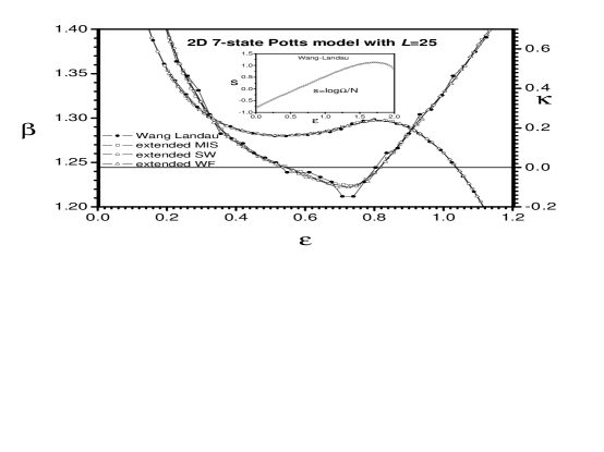
Figure 2: Microcanonical caloric and curvature curves associated with the $2D$ seven-state Potts model obtained from the application of the extended canonical MC algorithms (MIS: Metropolis importance sample, SW: Swendsen-Wang, and WF: Wolff’s clusters algorithm). Such results can be compared with the ones obtained from a direct numerical differentiation of the entropy per particle $s=\log\Omega/N$ obtained by using the Wang-Landau sampling method.

The results derived from the extended versions of the Metropolis importance sample, as well as the Swendsen-Wang and Wolff’s clusters algorithms are shown in FIG.2 for the particular case of the $2D$ seven-state Potts model with $L=25$. Each point of these dependencies have been obtained from MC runs with $10^{6}$ steps. For comparison purposes, we have also carried out the calculation of the caloric $\beta\left(\varepsilon\right)$ and the curvature $\kappa\left(\varepsilon\right)$ curves by performing a direct numerical differentiation of the entropy per particles $s(\varepsilon)=\log$ $\Omega(E)/N$ obtained from the Wang-Landau sampling method [35], which is shown in the inset panel ($N=L^{2}$). Although there exist a good agreement among all these MC results, the ones obtained from the Wang-Landau method seem to be less significant, overall, the results corresponding to the curvature curve $\kappa(\varepsilon)$.

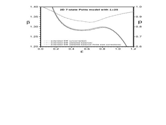
Figure 3: Microcanonical caloric curves $\beta\left(\varepsilon\right)$ showing the different corrections of finite size effects corresponding to the Swendsen-Wang clusters algorithm. We also show here the expectation value of the acceptance probability $p=\left\langle w_{i\rightarrow f}\right\rangle$ versus energy per particle $\varepsilon$ corresponding to the extended Swendsen-Wang algorithm obeying detailed balance.

The previous results constitute a clear illustration that the finite size corrections formulae introduced in subsection 2.2 provide a significant improvement in the precision of this kind of MC calculations. In this particular example with $L=25$, the contribution of first-order correction of finite size effects in the caloric curve $\beta\left(\varepsilon\right)$ have a typical order of $\delta_{1}\sim 10^{-3}$, while the one corresponding to the second-order correction are of order $\delta_{2}\sim 10^{-5}$. Nevertheless, the most significative correction of finite size effects in non-local canonical MC methods comes from the fulfilment of the detailed balance condition (54) obtained after the introduction of a posteriori acceptance probability (57), whose correction has a typical order of $\delta_{db}\sim 10^{-2}$. This fact can be appreciated in FIG.3 for the case of the Swendsen-Wang clusters algorithm.

Although the acceptance probability $w_{i\rightarrow f}$ for clusters flipping is lower than the unity, its expectation value $p=\left\langle w_{i\rightarrow f}\right\rangle$ is significantly high for most of energy region (see also in FIG.3). Since the consideration of such an a posteriori acceptance probability $w_{i\rightarrow f}$ corrects a finite size effect error $\delta_{\beta}=\left|\beta_{\omega}^{i}-\beta_{\omega}^{t}\right|$ associated with the estimation of the transition inverse temperature $\beta_{\omega}^{t}$, one should observe a growth of the expectation value $\left\langle w_{i\rightarrow f}\right\rangle$ as $N$ increases. Such a behavior is indeed appreciated in FIG.4 for the extended clusters algorithms. While all these dependencies have a similar qualitative behavior, the expectation value of the acceptance probability $\left\langle w_{i\rightarrow f}\right\rangle$ of the extended Wolff’s clusters algorithm in the paramagnetic region is larger than the one corresponding to the extended Swendsen-Wang method. This is a quite expected qualitative result. The acceptance probability $w_{i\rightarrow f}$ should correct in the first case the finite size error $\delta_{\beta}=\left|\beta_{\omega}^{i}-\beta_{\omega}^{t}\right|$ related to the flipping of only one cluster, while the finite size error $\delta_{\beta}$ related to the extended Swendsen-Wang method is larger due to this algorithm involves the flipping of all system clusters. At low energies or in the ferromagnetic region, these methods have practically the same performance, since the number of spins belonging to the cluster is comparable to the system size $N$ (see a more detailed comparison in the inset panel of FIG.4).

Figure 4: Size dependence of the expectation value of the a posteriori the acceptance probability $p=\left\langle w_{i\rightarrow f}\right\rangle$ for the extended clusters algorithms.

The qualitative behavior of the dependence $\left\langle w_{i\rightarrow f}\right\rangle$ versus $\varepsilon$ finds a simple explanation in terms of the explicit dependence of the acceptance probability $w_{i\rightarrow f}$ on the coupling constant $\lambda$. While the acceptance probability $w_{i\rightarrow f}\equiv 1$ within the canonical ensemble where $\lambda=0$, this quantity undergoes a reduction with the increase of the coupling constant $\lambda$. Moreover, the optimal value of coupling constant $\lambda_{\Delta}=\sqrt{1+\kappa^{2}}-\kappa$ employed in the present MC simulations increases with the reduction of the system curvature $\kappa$. Indeed, the lowest values of $\left\langle w_{i\rightarrow f}\right\rangle$ are observed in the energy region where the system curvature also exhibits its lower values, that is, the anomalous region with negative heat capacities $C<0$.

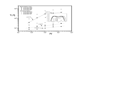
Figure 5: Main panel: Size dependence of the decorrelation time $\tau$ and the efficiency factor $\eta=\tau\Delta_{T}^{2}$ for the extended canonical MC simulations with environment inverse temperature $\beta_{\omega}(\varepsilon)=\beta_{e}+\lambda(\varepsilon-\varepsilon_{e})$. Here, $\beta_{e}=\beta_{pt}$, $\varepsilon_{e}=\varepsilon_{2}$, $\lambda=\lambda_{\Delta}\left(\kappa_{2}\right)$ and $\kappa_{2}=\kappa\left(\varepsilon_{2}\right)$, where $\beta_{pt}$ is the estimated inverse temperature that corresponds to the discontinuous PT, while $\varepsilon_{2}$ is the stationary solution derived from the thermal equilibrium condition $\beta(\varepsilon_{2})=\beta_{pt}$ located within the region with negative heat capacities $C<0$. Inset panel: Size dependence of the entropy per particle $s(\varepsilon)$, or more exactly, the quantity $s^{\ast}\left(\varepsilon\right)=s(\varepsilon)-\beta_{pt}\varepsilon+const$, which allows to show the convex intruder associated with the region with negative heat capacities. The energies corresponding to the two maxima $\left(\varepsilon_{1},\varepsilon_{3}\right)$ and the minimum $\varepsilon_{2}$ are the three stationary solutions derived from the thermal equilibrium condition $\beta\left(\varepsilon_{1,2,3}\right)=\beta_{pt}$.

The size dependencies of the decorrelation time $\tau$ and the efficiency factor $\eta=\tau\Delta_{T}^{2}$ within the anomalous region with $C<0$ are shown in the main panel of FIG.5. Due to computational limitations, the data were obtained from MC simulations with lattice sizes $L=\left(8,16,32,64,128\right)$. Since the absolute values of the curvature $\kappa$ are close to zero $\left|\kappa\right|\simeq 0$, the total dispersion is approximately given by the constant value $\Delta_{T}^{2}\simeq 2$, in accordance with Eq.(15). This is the reason why the dependencies $\tau(N)$ and $\eta(N)$ are almost displaced in a constant value along the vertical direction of the log-log graph shown in FIG.5.

As expected, the extended version of the Metropolis importance sample exhibits the largest values of the decorrelation time $\tau$ for the lattice sizes $L$ studied in this work. Curiously, the size dependence of its decorrelation time $\tau(N)$ shows an abrupt transition from a power-law regime with exponent $\alpha_{1}\simeq 0$.$72$ to other one with exponent $\alpha_{2}\simeq 0$.$14$ close to $N\simeq 10^{3}$ ($L=32$). Despite of the extended Metropolis importance sample is a local MC method, the effective exponent $\alpha_{2}$ for the larger system sizes is comparable to the ones associated with the extended clusters MC methods, $\alpha_{SW}\simeq 0$.$18$ (Swendsen-Wang) and $\alpha_{WF}\simeq 0$.$15$ (Wolff). Note also that the efficiency of these extended clusters methods are still significant despite of the consideration of the a posteriori acceptance probability (74) employed here to ensure the detailed balance condition (54).

The above examples confirm that the efficiency achieved with the application of the present methodology is more significant than the improvement considered by the application of re-weighting techniques such as multicanonical method and its variant, whose typical values of the exponent $\alpha$ ranges from 2 to 2.5 in the case of Potts models [34]. As already evidenced in FIG.2, while the Wang-Landau sampling method provides a good estimation of the entropy per particle $s(\varepsilon)$, its underlying statistical errors are still appreciable in the curvature curve $\kappa\left(\varepsilon\right)=-\partial^{2}s\left(\varepsilon\right)/\partial\varepsilon^{2}$ regardless the simulation was extended until the modifying factor fulfills the condition $f_{i}<\exp\left(10^{-10}\right)$. Such an observation evidences that the results obtained from this last method are not sufficiently relaxed to provide a precise estimation of the curvature curve $\kappa\left(\varepsilon\right)$. By considering the CPU time-cost needed to achieve the convergence, it is more convenient to perform a punctual estimation of the caloric $\beta\left(\varepsilon\right)$ and curvature $\kappa\left(\varepsilon\right)$ curves with any extended canonical MC method instead of carrying out a numerical differentiation of the microcanonical entropy $s(\varepsilon)$ over an energy range obtained from a re-weighting technics such as the Wang-Landau sampling method.

4 Conclusions

In this work, we have shown that the methodology to extend canonical MC methods inspired on the consideration of the recently obtained fluctuation relation (2) can be improved to account for the existence of finite size effects and to fulfil of the detailed balance condition (54). Remarkably, despite of the consideration of the a posteriori acceptance probability (57) reduces the efficiency of the clusters MC methods, it has been shown that the relaxation times needed to ensure the convergence are more significant than the ones achieved with re-weighting technics such as multicanonical methods and its variants. For the particular case of the seven-states Potts model, the consideration of any extended canonical MC algorithm enables a suppression of the super-critical slowing down associated with the occurrence of the temperature driven first-order phase transition of this model from an exponential growth to a very weak power-law dependence with exponent $\alpha=0.14-0.18$.

There is still some open questions in regard to the potentialities of the present methodology. For example, although this method has been specially conceived to overcome the slow relaxations of canonical MC simulations near to a region with a first-order phase transition, in principle, there is no limitation that the same one can be also employed to improve canonical MC simulations near to a critical point of a continuous phase transition. Moreover, a similar extension is possible to carry out for those MC methods based on the consideration of the Boltzmann-Gibbs distributions:

$$dp_{BG}(E,X)=\frac{1}{Z(\beta,Y)}\exp\left[-\beta(E+YX)\right]dEdX$$ (76)

to account for the existence of anomalous values in other response functions besides the heat capacity. The analysis of these questions deserve a special attention in future works.

References

- [1] Velazquez L and Curilef S, 2010 Journal Statistical Mechanics: Theory and Experiment P02002.
- [2] Padmanabhan T, 1990 Physics Reports 188 285.
- [3] Lynden-Bell D, 1999 Physica A 263 293.
- [4] Gross D H E, 2001 Microcanonical thermodynamics: Phase transitions in Small systems (66 Lectures Notes in Physics) (Singapore: World scientific).
- [5] Gross D H E and Madjet M E, 1997 Z. Phys. B 104 521.
- [6] Moretto LG, Ghetti R, Phair L, Tso K, Wozniak GJ, 1997 Phys. Rep. 287 250.
- [7] D’Agostino M, Gulminelli F, Chomaz P, Bruno M, Cannata F , Bougault R, Gramegna F, Iori I, Le Neindre N, Margagliotti GV, Moroni A and Vannini G, 2000 Phys. Lett. B 473 219.
- [8] Landau P D and Binder K, 2000 A guide to Monte Carlo simulations in Statistical Physics (Cambridge Univ Press).
- [9] Velazquez L and Curilef S, 2009 J. Phys. A: Math. Theor. 42 095006.
- [10] Velazquez L and Curilef S, 2009 J. Stat. Mech. P03027.
- [11] Velazquez L and Curilef S, 2009 J. Phys. A: Math. Theor. 42 335003.
- [12] Gerling A and Hüller R W, 1993 Z. Phys. B 90 207.
- [13] Thirring W, 1980 Quantum Mechanics of large systems (Springer) Ch. 2.3.
- [14] Reichl L E, 1998 A Modern Course In Statistical Physics (Wiley).
- [15] Challa M S S and Hetherington J H, 1988 in Computer Simulation Studies in Condensed Matter Physics I, Eds. D.P. Landau, K. K. Mon and H.-B. Schüttler (Heidelberg: Springer).
- [16] Hetherington J H, 1987 J. Low Temp. Phys. 66 145.
- [17] Costeniuc M, Ellis R S, Touchette H and Turkington B, 2005 J. Stat. Phys. 119 1283.
- [18] Toral R, 2006 Physica A 365 85.
- [19] Metropolis N, Rosenbluth A W, Rosenbluth M N, Teller A H and Teller E, 1953 J. Chem. Phys. 21 1087.
- [20] Hastings W K, 1970 Biometrika 57 97.
- [21] Swendsen R H and Wang J-S, 1987 Phys. Rev. Lett. 58 86.
- [22] Wang J-S, Swendsen R H and Kotecký R, 1989 Phys. Rev. Lett. 63 1009.
- [23] Wolff U, 1989 Phys. Rev. Lett. 62 361.
- [24] Edwards R G and Sokal A D, 1988 Phys. Rev. D 38 2009.
- [25] Niedermayer F, 1988 Phys. Rev. Lett. 61 2026.
- [26] Evertz H G, Hasenbusch M, Marcu M, Pinn K and Solomon S, 1991 Phys. Lett. B 254 185.
- [27] Hasenbusch M, Marcu M and Pinn K, 1994 Physica A 211 255.
- [28] Dress C and Krauth W, 1995 J. Phys. A 28 L597.
- [29] Liu J W and Luijten E, 2004 Phys. Rev. Lett. 92 035504.
- [30] Kasteleyn P W and Fortuin C M, 1969 J. Phys. Soc. Japan Suppl. 26s 11.
- [31] Fortuin C M, and Kasteleyn P W, 1972 Physica 57 536.
- [32] Wu F Y, 1982 Rev. Mod. Phys. 54 235.
- [33] Viana Lopes J et al, 2006 Phys. Rev. E 74 046702.
- [34] Berg B and Neuhaus T, 1991 Phys. Lett. B 267 249; 1992 Phys. Rev. Lett. 68 9.
- [35] Wang F and Landau D P, 2001 Phys. Rev. Lett. 86 2050; Phys. Rev. E 64 056101.