On the orbital evolution of a giant planet pair embedded in a gaseous disk. I: Jupiter-Saturn configuration

Abstract

We carry out a series of high resolution ($1024\times 1024$) hydrodynamical simulations to investigate the orbital evolution of Jupiter and Saturn embedded in a gaseous protostellar disk. Our work extends the results in the classical papers of Masset & Snellgrove (2001) and Morbidelli & Crida (2007) by exploring various surface density profiles ($\sigma$), where $\sigma\propto r^{-\alpha}$. The stability of the mean motion resonances(MMRs) caused by the convergent migration of the two planets is studied as well. Our results show that:(1) The gap formation process of Saturn is greatly delayed by the tidal perturbation of Jupiter. These perturbations cause inward or outward runaway migration of Saturn, depending on the density profiles on the disk. (2) The convergent migration rate increases as $\alpha$ increases and the type of MMRs depends on $\alpha$ as well. When $0<\alpha<1$, the convergent migration speed of Jupiter and Saturn is relatively slow, thus they are trapped into 2:1 MMR. When $\alpha>4/3$, Saturn passes through the $2:1$ MMR with Jupiter and is captured into the $3:2$ MMR. (3) The $3:2$ MMR turns out to be unstable when the eccentricity of Saturn ($e_{s}$) increases too high. The critical value above which instability will set in is $e_{s}\sim 0.15$. We also observe that the two planets are trapped into $2:1$ MMR after the break of $3:2$ MMR. This process may provide useful information for the formation of orbital configuration between Jupiter and Saturn in the Solar System.

1 Introduction

Planet-planet interaction within an environment of gas disk is an important procedure that may account for the initial conditions of multiple planet system after the depletion of gas disk, and thus affects their final orbital configurations. One of the notable configuration that two planets may achieve is the mean motion resonance (MMR). For example, the crossing of 2:1 MMR between Jupiter and Saturn was proposed to account for the later heavy bombardments of the Solar system(Tsiganis et al., 2005; Gomes et al., 2005). MMRs are also common in the recently detected exoplanets. Among the $\sim 45$ detected multiple exoplanet systems, at least 7 planet pairs are believed to be trapped in low order MMRs (see Table 1 for a list).

According to the general theory of disk-planet interaction, a single planet embedded in a gaseous disk may undergo various types of migration. For a planet with mass smaller than several Earth masses ($M_{\oplus}$), the angular momentum exchange between it and the gas disk will cause a net momentum loss on the planet and results in a fast orbit decay, which is called type I migration(Goldreich & Tremaine, 1979; Ward, 1997). For a planet with mass comparable to Jupiter, it opens a gap around its orbit. Through the planet, the angular momentum exchange between the outer and inner part of the disk balances each other. This effect locks the planet and forces it to move as a part of the disk, at the viscous evolution timescale. This is called the type II migration (Lin & Papaloizou, 1986). Moderate mass planets(comparable to Saturn) may undergo very fast migration, which is believed to be caused by the large corotation torque risen from the perturbed coorbital zone of the planet. It is now named runaway migration or type III migration with timescale of several tens of orbit periods only(Masset & Papaloizou, 2003).

Due to the different migration rates of two planets embedded together in a disk, MMRs may be established through the relative convergent migration. For example, when the outer planet is less massive than the inner one and undergoes type I or III migration, it will probably catch up the more massive inner one which undergoes type II migration, even they are both migrating at the same direction. So, in multiple planet systems with heavier planet locating at the inner side, planets may be easily trapped into the MMRs. Many constructive studies have been made to investigate this scenario, either by three-body simulations with prescribed disk effects, e.g., Snellgrove et al. (2001) and Nelson & Papaloizou (2002), or through hydrodynamic simulations, e.g., Papaloizou & Szuszkiewicz (2005), Kley et al. (2004, 2005) and Pierens & Nelson (2008).

Masset & Papaloizou (2003) investigated a case where the Jupiter(inner)-Saturn(outer) pair embedded in a protostellar disk. In that case, Saturn migrates inward very fast(type III migration) and is then captured into $3:2$ MMR by Jupiter which undergoes slow type II migration. As soon as the resonance is well established, the two planets reverse their migration and move outward together, preserving their resonance. Morbidelli & Crida (2007) confirmed these results by using a more reliable code that describes the global viscous evolution of the disk. They considered a wide set of initial conditions and found the $3:2$ MMR is a robust outcome of Jupiter-Saturn pair, which is compatible to the requirement of a compact initial configuration of Jupiter and Saturn (with period ratio slightly less than 2). After gas depletion, the subsequent 2:1 MMR crossing under the interaction with planetesimal disk may achieve the present configuration of Solar system(Tsiganis et al., 2005; Gomes et al., 2005; Morbidelli et al., 2005).

Morbidelli & Crida (2007) also showed that, the common migration rate of Jupiter and Saturn depends on the viscosity of the disk, as well as vertical scale height ($H/r$) of the gas disk. At $H/r=0.05-0.06$, Jupiter and Saturn seem to be in a quasi-stationary configuration without migration. With such conditions, Morbidelli et al. (2007) found that, the Jupiter-Saturn pair could maintain the $3:2$ MMR for at least $1500$ Jovian orbital periods when the gas disk dissipating slowly and smoothly. And we note that, through their evolutions, the eccentricities of Jupiter and Saturn stay at relatively low values($e<0.05$).

In this paper, following the work of Masset & Snellgrove (2001) and Morbidelli & Crida (2007), we investigate the orbital evolution of Jupiter-Saturn pair embedded in gas disk with different slope of surface density ($\alpha$), i.e., $\alpha=-\ln(\sigma)/\ln(r)$. We will show that, under suitable disk condition, $\alpha\geq 4/3$ (or $<1$), Jupiter and Saturn will undergo outward (or inward) migration after trapped into $3:2$ (or $2:1$, respectively) MMRs. Thus the surface density profile plays an important role on determining the type of resonance and their consequent migrations. Also we will show that, under some circumstances, the eccentricities of Jupiter and Saturn will be excited up to 0.15 along the migration. The eccentricity excitation and subsequent stability of the MMRs between Jupiter and Saturn are discussed. Such a study help us to reveal the orbital architecture formation of our Solar system.

Our paper is organized as follows: in Section 2 we describe our model including the numerical methods and the initial settings. In Section 3 we present our results as well as the analysis. The conclusions and discussions will be placed at Section 4.

2 Model and Numerical Set up

2.1 Physical model

Following conventional procedures, we simulate the full dynamical interaction of a system includes a solar type star, two giant protoplanets and a 2-dimensional (2D) gas disk. The star is fixed at the origin of the system with both the planets and disk surrounding it. We denote the inner and outer planets with subscript 1 and 2, respectively.

For numerical convenience, the gravitational constant $G$ is set to be $1$. The Solar mass ($M_{\odot}$) and the initial semi-major axis of inner planet ($R_{10}=5.2$ AU) are set as the units of mass and length, respectively. Then the unit of time is $\frac{1}{2\pi}P_{10}$, where $P_{10}$ the initial period of inner orbit. The mass of central star is set to be 1 Solar mass ($M_{*}=1M_{\odot}$).

We solve the continuity and momentum equations of the gas disk in 2-D space, neglecting the self-gravity of the gas. In order to properly describe the global viscous evolution of the whole disk and to avoid the annoying inner boundary, we employ a Cartesian grid. The vertically averaged continuity equation for the gas is given by

$$\frac{\partial\sigma}{\partial t}+\frac{\partial(\sigma u_{x})}{\partial x}+\frac{\partial(\sigma u_{y})}{\partial y}=0,$$ (1)

where $\sigma$ is the surface density. The equations of motion in the Cartesian coordinates are

$$\frac{\partial(\sigma u_{x})}{\partial t}+\frac{\partial(\sigma u_{x}^{2})}{\partial x}+\frac{\partial(\sigma u_{x}u_{y})}{\partial y}=-\frac{\partial P}{\partial x}-\sigma\frac{\partial\Phi}{\partial x}+\frac{\partial Q_{xx}}{\partial x}+\frac{\partial Q_{xy}}{\partial y},$$ (2)

$$\frac{\partial(\sigma u_{y})}{\partial t}+\frac{\partial(\sigma u_{x}u_{y})}{\partial x}+\frac{\partial(\sigma u_{y}^{2})}{\partial y}=-\frac{\partial P}{\partial y}-\sigma\frac{\partial\Phi}{\partial y}+\frac{\partial Q_{xy}}{\partial x}+\frac{\partial Q_{yy}}{\partial y},$$ (3)

where $P$ is the pressure and $\Phi$ is the gravity potential of the whole system. $\Phi$ includes the softened potential of the central star $\Phi_{*}$, softened potential of the giant planets ($\Phi_{p,1}$,$\Phi_{p,2}$) and the indirect potential $\Phi_{\rm ind}$ rises from the acceleration of the origin, which is caused by the planets and the gas disk. We adopt a softened gravity potential of the central star to avoid the singularity at the very center of the computational domain,

$$\Phi_{s}=-\frac{GM_{\odot}}{\sqrt{x^{2}+y^{2}+\epsilon_{*}^{2}}}.$$ (4)

The potential of each planet is also softened,

$$\Phi_{p,i}=-\frac{GM_{p,i}}{\sqrt{(x-x_{p,i})^{2}+(y-y_{p,i})^{2}+\epsilon_{p}^{2}}},~{}~{}(i=1,2),$$ (5)

where $\epsilon_{*}$ and $\epsilon_{p}$ are the soften length to the central star and planets respectively. We test several values of $\epsilon_{*}$ and set it to be $0.05$ for the balance of efficiency and accuracy. The $\epsilon_{p}$ is set to be $0.6H$, where $H$ is the scale height of the gas disk.

The viscosity of gas is carried out by solving the stress tensors $Q_{xx}$, $Q_{yy}$ and $Q_{xy}$ explicitly:

$$Q_{xx}=2\eta[\frac{\partial u_{x}}{\partial x}-\frac{1}{3}(\frac{\partial u_{x}}{\partial x}+\frac{\partial u_{y}}{\partial y})],$$ (6)

$$Q_{yy}=2\eta[\frac{\partial u_{y}}{\partial y}-\frac{1}{3}(\frac{\partial u_{x}}{\partial x}+\frac{\partial u_{y}}{\partial y})],$$ (7)

$$Q_{xy}=\eta(\frac{\partial u_{x}}{\partial y}+\frac{\partial u_{y}}{\partial x}).$$ (8)

where $\eta=\sigma\nu$ and $\nu$ is the dynamical viscous coefficient of the gas, which is assumed to be constant all over the disk.

We assume the disk gas has a polytropic equation of state:

$$P=K\sigma^{\gamma},$$ (9)

where $\gamma=\frac{5}{3}$. $K$ is a constant that makes the following equation satisfied at $r=1$,

$$c_{s}(r)=\sqrt{\frac{\partial P}{\partial\sigma}}=\left(\frac{H}{r}\right)v_{\rm kep}|_{r=1},$$ (10)

where $c_{s}(r)$ is the speed of sound and $v_{\rm kep}(r)$ is the Keplerian velocity of the gas. According to our settings and units, $K=0.1349$. To focus on the effects of the surface density distribution, we fix the disk viscosity $\nu=10^{-6}$ and the disk aspect ratio $H/r=0.04$. The planetary accretion and self-gravity of gas disk are neglected to reduce variables and to improve the computational efficiency.

2.2 Mesh configuration and computational domain

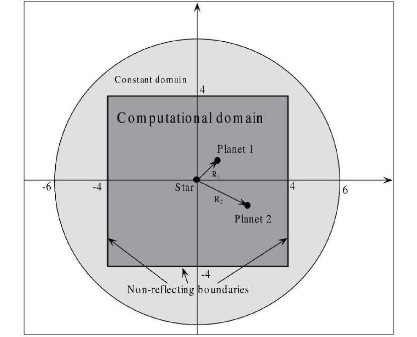
Figure 1: The computational domain is from -4 to 4 in x direction and from -4 to 4 in y direction(gray square). Surrounding it are four non-reflecting boundaries. Area outside the square is assumed to stay constant. We take the gravity comes from the whole round area($R\leq 6$) as a background potential which is a function of radius.

The Antares code we have developed is adopted in the simulations. It is a 2D Godunov code based on the exact Riemann solution for isothermal or polytropic gas, featured with non-reflecting boundary conditions. The detail of this method was described elsewhere(Yuan & Yen, 2005). Since we adopt the Cartesian grids, the computational domain is also a square. Figure 1 shows the computational domain. To get the proper gravity potential of a disk, we add an circular area outside the computational domain. Since it is far from the interested place, this circular area stays at the initial condition during the simulations and its gravity potential is pre-calculated. The computational domain (gray area) is divided by a Cartesian mesh. The resolution of this mesh is a crucial issue for hydrodynamics simulations, since poor resolution may introduce non-physical effects that affects the migration of planets greatly. So we employ a high resolution: $N_{x}\times N_{y}=1024\times 1024$. The real computational time for a single 2000-orbits run is $3-4$ weeks, in a full parallelized 64-cpus cluster. This almost reaches the upper limit of normal computational ability, and the higher resolution may be achieved by the nested grids or other technics.

The reasons and advantages of our choosing of Cartesian grids had been discussed in our previous paper(Zhang et al., 2008). For the orbits of two planets we integrate a three-body problem associate with the potential of gas disk by adopting a 8th-order Runge-Kutta integrator. The global time step is set as the minimum of the hydrodynamical and the orbital integration part.

2.3 Corner-Transport Correction

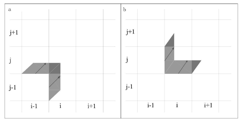
Figure 2: The real flux flows at an angle to the grid lines(assume $u_{x}>0,u_{y}>0$). (a) The new value $Q^{n+1}_{i,j}$ in cell $(i,j)$ should also be affected by the old value $Q^{n}_{i-1,j-1}$ in cell $(i-1,j-1)$. (b) The flux at four interfaces of cell $(i,j)$ need additional corrections—see the four dark triangles.

Although it is easy to implement, the Cartesian grids have a disadvantage to simulate a circularly orbiting gas disk, where the physical stream lines are neither parallel nor perpendicular to either of the grid lines in x- and y-directions. The flux is evaluated at each interface at which the velocity of gas projects to the coordinate directions. When the grid resolution is low, the conservative law may break along the grid lines(see Figure 2) and much dissipation arise. It is a kind of numerical viscosity which reaches maximum at the diagonal area of the computational domain. To make this numerical viscosity negligible, the resolution of the grids usually needs to be very high. Instead, we adopt the CTU(Corner-Transport Upwind) method to minimize this grid effect at the resolution that we can achieve so far.

Following the CTU method, we add correcting terms to the flux at each interface of all cells. The value of this correcting flux depends on the angle between the direction of the physical velocity and the grid lines. As Figure 2 shows, by assuming $u_{x}>0$ and $u_{y}>0$, the cell $(i,j)$ is affected by an additional flux comes from cell $(i-1,j-1)$. The cell averaged value $Q^{n+1}_{i,j}$, for example, is modified by a term,

$$\frac{\frac{1}{2}u_{x}u_{y}(\Delta t)^{2}}{\Delta x\Delta y}(Q^{n}_{i-1,j}-Q^{n}_{i-1,j-1}),$$ (11)

where $\frac{1}{2}u_{x}u_{y}(\Delta t)^{2}$ is the area of the small triangular portion moving into cell $(i,j+1)$ and $\Delta x\Delta y$ is the area of the cell in which the jump $Q^{n}_{i,j}-Q^{n}_{i-1,j}$ is averaged. The corresponding fluxes evaluated at the four interfaces of cell $(i,j)$ now read

$$\begin{split}F_{i-\frac{1}{2},j}=F_{i-\frac{1}{2},j}-\frac{1}{2}\frac{\Delta t}{\Delta y}u_{x}u_{y}(Q^{n}_{i-1,j}-Q^{n}_{i-1,j-1}),\\ F_{i+\frac{1}{2},j}=F_{i+\frac{1}{2},j}-\frac{1}{2}\frac{\Delta t}{\Delta y}u_{x}u_{y}(Q^{n}_{i,j}-Q^{n}_{i,j-1}),\\ G_{i,j-\frac{1}{2}}=G_{i,j-\frac{1}{2}}-\frac{1}{2}\frac{\Delta t}{\Delta y}u_{x}u_{y}(Q^{n}_{i,j-1}-Q^{n}_{i-1,j-1}),\\ G_{i,j+\frac{1}{2}}=G_{i,j+\frac{1}{2}}-\frac{1}{2}\frac{\Delta t}{\Delta y}u_{x}u_{y}(Q^{n}_{i,j}-Q^{n}_{i-1,j}).\end{split}$$ (12)

The details and implementations of CTU method for conservation laws have been well discussed by Colella (1990).

2.4 Comparison with other codes

To ensure the reliability of our code, we performed a series of comparisons with other representative codes, e.g. FARGO. We examined the gap opening by Jupiter in a 2D gas disk. The physical setups and initial conditions are the same with that adopted by de Val-Borro et al. (2006), except that our radial domain is from $0$ to $2.5$ instead of $[0.4,2.5]$. The grid resolution is $640\times 640$ in the spatial range of $[x_{min},x_{max}]\times[y_{xmin},y_{max}]=[-2.5,2.5]\times[-2.5,2.5]$. Following their descriptions, we focus on the density contours of the gap, the evolution of density profiles, the evolution of total mass and the torques exerted on Jupiter. All the comparisons are performed in both inviscid and viscous disk, where the dynamical viscous coefficient is set to be $\nu=0$ and $\nu=10^{-5}$ respectively. The results with which we compared ourselves are obtained from the web which maintained by de Val-Borro.

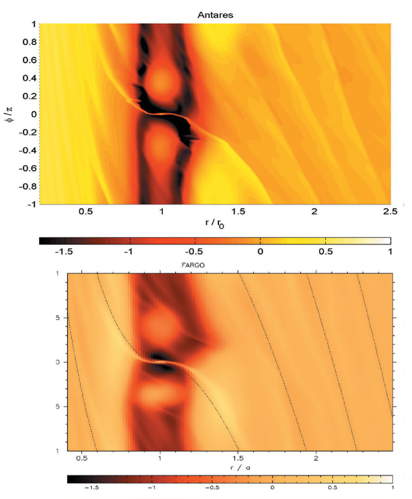
Figure 3: Density maps in logarithmic scale after 100 orbits for the inviscid simulations. Note that the computational domain of Antares is $(r_{min},r_{max})=(0,2.5)$, instead of $(0.4,2.5)$. The density range is $-1.7<\log(\sigma/\sigma_{0})<1$. Antares adopts isothermal equation of state(EOS) instead of the locally isothermal EOS, so the pitch angle is bit large than that in FARGO. The results of FARGO are obtained from the web: http://www.astro.su.se/groups/planets/comparison, which is maintained by de Val-Borro.

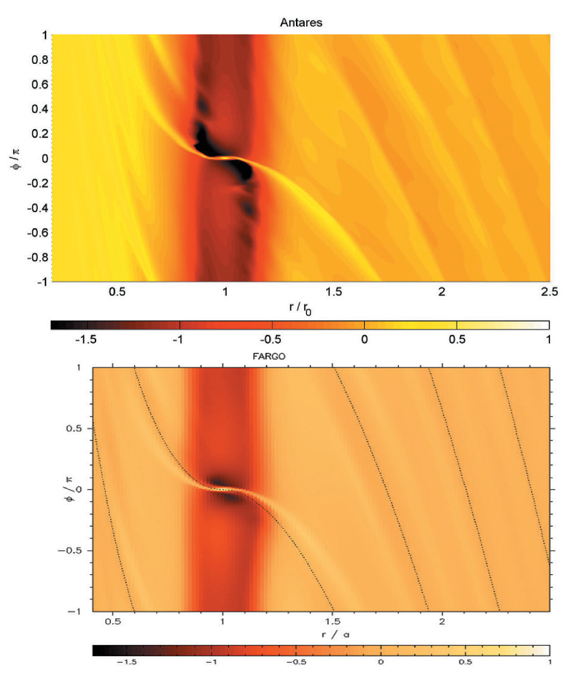
Figure 4: Density maps in logarithmic scale after 100 orbits for the viscous simulations. The viscous coefficient $\nu=10^{-5}$. The density range is also $-1.7<\log(\sigma/\sigma_{0})<1$. The results of FARGO are obtained from the web: http://www.astro.su.se/groups/planets/comparison, which is maintained by de Val-Borro.

Figure 3 shows the density contours after 100 orbits for the inviscid simulation. Two shocks are observed in our simulation (Antares): the primary one starts from the planet’s location and the secondary one starts near the $L_{5}$ point. We find the pattern of the spiral arms are similar with that of the other codes although the pitch angle of the primary arm(outside the orbit of planet) is a bit higher in our simulation, which is probably caused by the relative large sound speed their. Since the exact Riemann solution is not valid for locally isothermal gas, we adopt the full isothermal equation of state in this comparison tests instead and set the sound speed $c_{s}=\frac{H}{r}v_{kep}|_{r=1}$, where $H$ is the height of disk and $v_{kep}$ is the Keplerian orbit speed. In the gap, there are two symmetric density enhancements locate close to the $L_{4}$ and $L_{5}$ points at azimuthal distance $\Delta\phi=\pm\pi/3$ from the planet’s location. This is in good agreement with the theoretical prediction and the results of FARGO. We also notice there is a density bump, which indicates the congregation of vortensity, orbiting along the outer edge of the gap, which is observed in many other codes as well, e.g. the results of FARGO and NIRVANA-GDA(de Val-Borro et al., 2006). In the viscous simulation, the gap opened by the planet is narrower and smoother(Figure 4). The density enhancements seen at the Lagrangian points inside the gap in the inviscid simulation are dissipated, so is the density bump at the outer edge of the gap. Our simulation presents the same results with the other codes and shows more detailed structures within the gap.

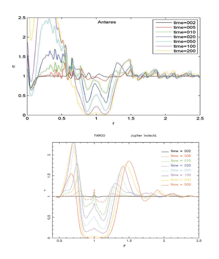
Figure 5: The normalized surface density profiles averaged azimuthally over $2\pi$ after 100 orbits for the inviscid simulations. Note that the computational domain of Antares is $(r_{min},r_{max})=(0,2.5)$, instead of $(0.4,2.5)$. The surface density at inner disk increases and keeps a high level when the inner open boundary is absent. The results of FARGO are obtained from the web: http://www.astro.su.se/groups/planets/comparison, which is maintained by de Val-Borro.

Figure 5 and 6 show the density profiles at different times in the inviscid and viscous simulations respectively. The width and depth of the gap in our simulations are in good agreement with those in FARGO. Our code also present the proper diffusion effects—decreasing on both the width and depth of the gap in viscous simulation. The major difference is the density on the inner disk: the surface density on the inner disk increases to higher value in our simulation than that in FARGO. This mainly comes from the different treatments at the center of disk.

As the Cartesian grids are adopted, we need not introduce any inner boundary at the center of disk but just let the gas accumulate there. The competition between the increasing pressure, the dissipation of gas and the gravity of central star(there also could be the accretion of the central star which is not included in this comparison simulation) will result in an equilibrium and maintain an inner structure naturally(whose scale is around $r\leq 0.1$ and changes with time). In a real proto-stellar disk, there probably exists an inner boundary near the center of disk, however it should be maintained by some equilibriums, e.g. the evaporation and the refilling of gas, and should move inward or outward according to the changes of local situation, e.g. the enhancement of the density, instead of a fixed boundary. And further more, a full inner disk(includes the part $r<0.4$) plays a great role on the dynamical interaction between the giant planet and the global disk, and thus can not be ignored without careful treatments(Crida et al., 2008).

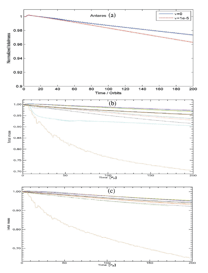
Figure 7: The evolution of total mass contained in the disk. (a) Total mass of disk calculated by Antares in inviscid and viscous simulations. (b) Total mass calculated by other codes in inviscid simulations. The legend details were presented in de Val-Borro (2006). (c) Total mass calculated by other codes in viscous simulations. See de Val-Borro (2006) again for legend details.

Compared to the codes adopt absorbing or open inner boundary, our code maintains relative high level of the total mass in the disk during the simulation. After $200$ orbits evolution, the total mass in our simulation decreases only $\sim 2.5\%$ for the inviscid case and $\sim 3.5\%$ for the viscous case. While most results of the other codes are at the range of $2\%-9\%$ for the inviscid simulations and $5\%-8\%$ for the viscous simulations(see Figure 7).

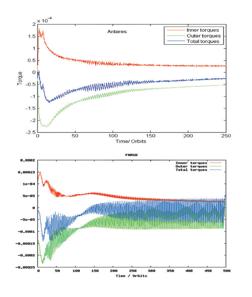
Figure 8: Comparison of the time-averaged torques exerted on Jupiter in inviscid simulations. The results of FARGO are obtained from the web: http://www.astro.su.se/groups/planets/comparison, which is maintained by de Val-Borro.

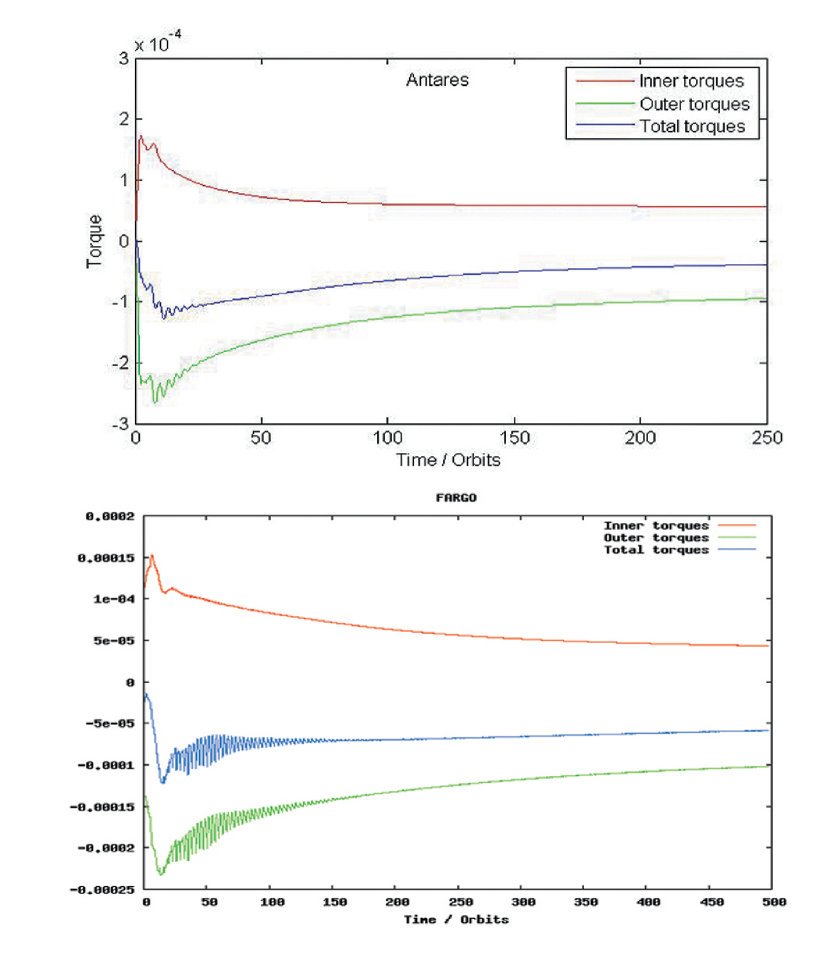
Figure 9: Comparison of the time-averaged torques exerted on Jupiter in viscous simulations. The viscosity coefficient is $\nu=10^{-5}$. The results of FARGO are obtained from the web: http://www.astro.su.se/groups/planets/comparison, which is maintained by de Val-Borro.

The comparisons of torques are showed in Figure 8 (inviscid) and Figure 9 (viscous). Our results are coherent well with FARGO both qualitatively and quantitatively. The averaged total torque between $175-200$ is $-2.5\times 10^{-5}$ in the inviscid simulation and $-6.6\times 10^{-5}$ in the viscous simulation. Both of this two values are around the average of the results presented by de Val-Borro et al. (2006).

According to the above comparisons, we conclude that our code—Antares—is reliable for simulating planet-disc interaction in Cartesian grids. By adopting the CTU method and high resolution mesh, the numerical dissipation (or grid effects) is negligible in our simulations.

2.5 Initial Conditions

The surface density of the gas disk ($\sigma$) varies as a function of its radius $r$. As shown in Table 2, we adopt several different initial distributions: $\sigma_{0}$, $\sigma_{0}e^{-r^{2}/53}$, $\sigma_{0}r^{-1/2}$ and so on. $\sigma_{0}$ is set to be 0.0006 in our units, which corresponds to a height-integrated surface density $\sim 200{\rm~{}g/cm}^{2}$. The angular velocity of the gas $u_{\theta}=r\Omega_{g}$ is slightly different from the Keplerian velocity since the flow is in a centrifugal balance with both the softened gravity of the star and the gas pressure which raises from the distribution of the surface density $\sigma(r)$. The initial radial velocity of gas is set to be 0. These initial conditions of the disk do not take into account of the gravitational perturbation by the planets.

To set up a dynamical equilibrium in which the orbit of a planet is circular and the stream lines are closed, we adopt an negligible initial mass for each of the planets ($3\times 10^{-7}$ or equivalently 0.1$M_{\oplus}$). And at the very first 200 fixed circular orbits, both growth rates of the planets are specified to be $\sim 3.5\%$ per orbit until they achieve the mass of Jupiter and Saturn, respectively. With this “quiet-start” prescription, the planets gain their masses through adiabatic growth so that the disk has enough time to make a smooth response. The releasing consequence of the two planets is a complicate issue, since it directly relates to the formation consequence of a multiple planet system. We choose to release two planets at the same time, so the pre-formed planet should stay at an circular orbit and wait for the later one. Although this process may introduce some inconsistences, it’s the most suitable initial state to investigate the migration of a planet pair.

3 Results

3.1 Effects of disk’s surface density

We consider a configuration in which Saturn locates outside the orbit of Jupiter, which is similar to our Solar system. As shown in Masset & Snellgrove (2001), this configuration usually leads to the convergent migration and resonance trapping in a gas disk. In this paper we focus on the effects of the disk’s surface density. The slope of the surface density determines the magnitudes of torques exerted on the planets, and thus affects the speed of the convergent migration as well as the type and stability of MMRs. We assume the surface density of disk is a function of its radii only: $\sigma=\sigma_{0}r^{-\alpha}$ and obtain a series of density distributions by varying the value of $\alpha$. As summarized by Table 2, most of the typical $\alpha$ had been considered: for example, a flat disk $\sigma=\sigma_{0}$, a moderate steep disk $\sigma=\sigma_{0}r^{-1}$ and some extreme steep ones, e.g. $\sigma=\sigma_{0}r^{-5/3}$.

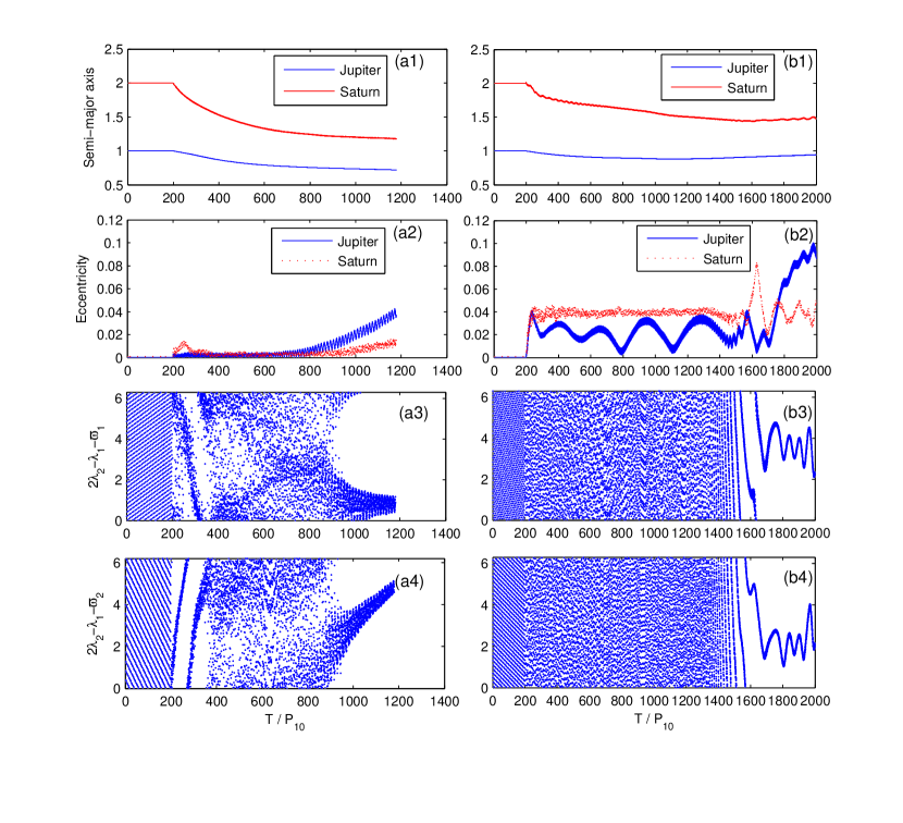
Figure 10: Orbital evolutions of Jupiter and Saturn embedded in a flat disk where $\sigma=\sigma_{0}r^{0}$ (Panels a1-a4) and a nearly flat disk where $\sigma=\sigma_{0}e^{-r^{2}/53}$ (Panels b1-b4), respectively. (a1) and (b1) Evolutions of the semi-major axes of the planets. The two planets approach to each other gently in a flat disk or a nearly flat disk. The common migration stops or even reverses after the establishment of resonance. (a2) and (b2) Evolutions of the eccentricities of planets. (a3) and (a4) Evolution of the resonance angles:$\theta_{1}=2\lambda_{2}-\lambda_{1}-\varpi_{1}$ and $\theta_{2}=2\lambda_{2}-\lambda_{1}-\varpi_{2}$ of $2:1$ MMR. (b3) and (b4) Evolution of the resonance angles: $\theta_{1}=2\lambda_{2}-\lambda_{1}-\varpi_{1}$ and $\theta_{2}=2\lambda_{2}-\lambda_{1}-\varpi_{2}$ of $2:1$ MMR. (A color version of this figure is available in the online journal.)

We start with a flat disk, where the initial surface density is $\sigma_{0}=0.0006$ which corresponds to a height-integrated surface density $\sim 200{\rm~{}g/cm}^{2}$. Panels (a1-a4) in Figure 10 show the evolutions of the semi-major axes, eccentricities and resonant angles of the two giant planets. When we release them at $t=200P_{10}$, Jupiter had almost opened a gap and begins a slow type II migration after a short transition period. While the situation is quite different for Saturn: the tidal torque generated by Jupiter keeps pushing the gas into the coorbital zone of Saturn, thus greatly delays the gap opening process of Saturn. As a result, Saturn migrates inward under the Lindblad and corotation torques, at a speed much faster than that of Jupiter. After the convergent migration, Saturn is trapped into the $2:1$ MMR with Jupiter. The eccentricities of both planets are excited as soon as the MMR is established.

Following the flat disk, we run a moderate case in which the surface density of disk is set to be $\sigma\sim e^{-\frac{r^{2}}{53}}$. This density profile is derived from the analysis of Guillot et al. (2006) for an evolving disk. It is in fact very close to the flat disk in our computational region($r\in(0,4)$). Embedding in this kind of disk, the migration of Saturn is a little more oscillatory than that in a flat disk, and we found the two planets stop and slightly reverse their migration to outward after they had been locked into the $2:1$ MMR. These are in good agreement with the results of Morbidelli & Crida (2007) at the similar parameter settings(the same disk aspect ratio, viscosity and surface density profile), as shown in the Panels (b1-b4) of Figure 10.

When the disk has a steep density profile, the situation becomes more complex. According to our simulations, different values of $\alpha$ lead to different rates of convergent migration, thus results in the trap of different MMRs. The common migration speed and direction also depend on the slope of disk density. We will state them in details as follows.

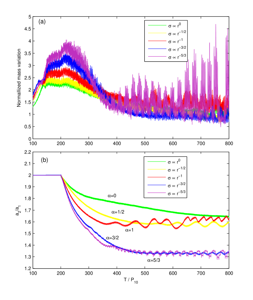
Figure 11: (a) Mass variation in the coorbital zone of Saturn during the convergent migration stage. It decreases when $\alpha$ decreases ($\sigma\propto r^{-\alpha}$)—from the top to the bottom in this panel, respectively. The radii of coorbital region is set to be $1.5R_{Hill}$ and the mass variation is normalized by the initial mass contains in Saturn’s coorbital region. (b) The different convergent migration rates with various $\alpha$: it increases at large $\alpha$. The convergent migration is halted when the two planets are locked into MMRs($2:1$ for $\alpha\leq 1$ and $3:2$ for $\alpha>1$). Note that mass variation decreases as the common gap forms. In Panel (a), the large variations in the curve of $\sigma\propto r^{-5/3}$ when $T>400P_{10}$ are the results of the increasing eccentricity of Saturn. This corresponds to the oscillations of the convergent migration($\alpha=5/3$) in Panel (b). (A color version of this figure is available in the online journal.)

First, the rate of convergent migration before the trapping of MMR increases as the density slope $\alpha$ increases, as shown in Panel (b) of Figure 11. After the moment of release ($t=200P_{10}$), the coorbital zone of Saturn is perturbed heavily by the density waves generated by Jupiter. The migration of Saturn is thus dominated by the corotation torque, which scales with the gradient of the potential vorticity within the vicinity of the planet in the linear approximation(Goldreich & Tremaine, 1979; Ward, 1991, 1992):

$$\Gamma_{C}\propto\sigma\frac{d\log{(\sigma/B})}{d\log{r}},$$ (13)

where $B=\kappa^{2}/(4\Omega)$ is the second Oort constant with $B\sim r^{-3/2}$ in a nearly Keplerian disk, and $\sigma=\sigma_{0}r^{-\alpha}$ is the surface density. So the direction and magnitude of the corotation torque, $\Gamma_{C}\propto(\frac{3}{2}-\alpha)r^{-\alpha}$, depends on $\alpha$. In fact, when the planet is forced to migrate fast (e.g., scattered by other planets) or its coorbital zone is perturbed heavily (in our cases, for example, the density waves generated by Jupiter), the density gradient in its coorbital zone is not monotone with $r$ and usually very complex. So the corotation torque exerted on it should be evaluated by the real angular momentum exchanged within the coorbital zone. Masset & Papaloizou (2003) found a relation between the dramatic migration rate and the coorbital mass deficit $\delta m$. In a Keplerian disk it reads:

$$\frac{1}{2}a\Omega(M_{p}-\delta m)\dot{a}=\Delta\Gamma_{LR}-\frac{\pi a^{2}\delta m}{3x_{s}}\ddot{a},$$ (14)

where $\Omega$ is the angular velocity of the planetary Keplerian motion, $M_{p}$ is the planet mass, $\Delta\Gamma_{LR}$ is the differential Lindblad torque and $x_{s}$ is the half-width of planet coorbital zone. A runaway migration occurs when $\delta m$ becomes comparable to the mass of planet $M_{p}$, because large $\delta m$ leads to fast migration which breaks the assumption that $a$ stays constant and results in an instability(Masset & Papaloizou, 2003). In our simulations, the steeper density profile between the orbits of Jupiter and Saturn results in heavier density waves that affect the coorbital zone of Saturn, and therefore, generates greater $\delta m$. Panel (a) in Figure 11 shows that the mass variation in the coorbital zone of Saturn increases at larger $\alpha$.

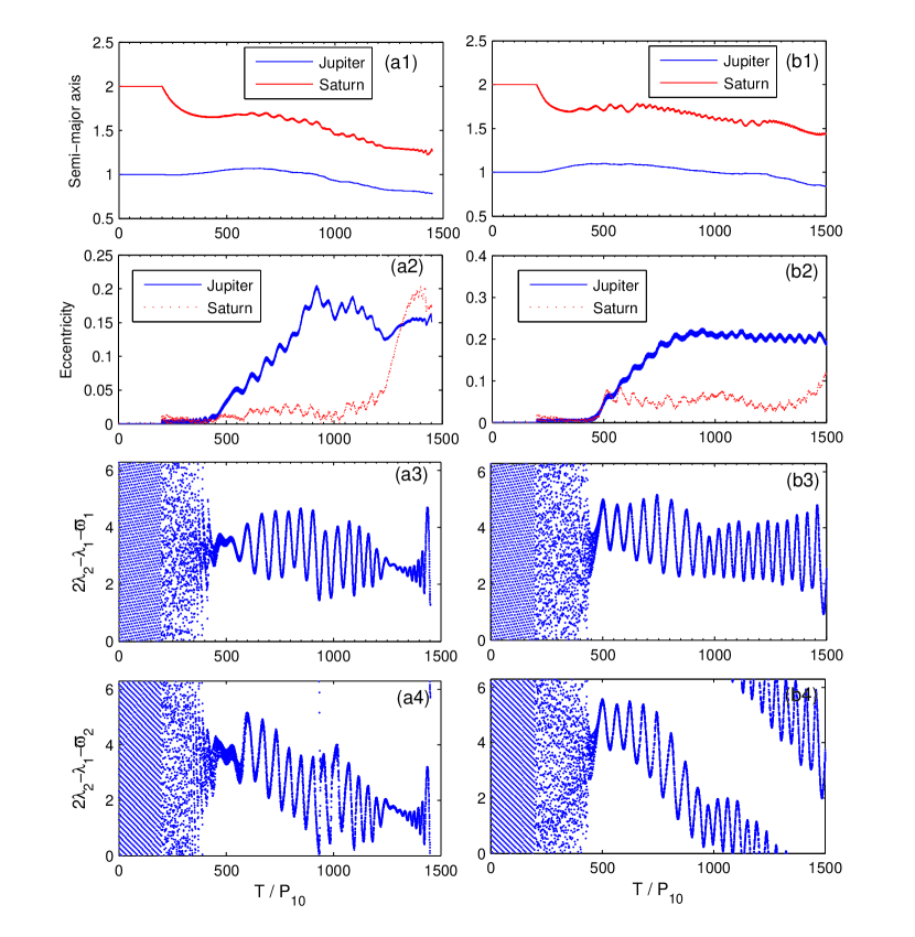
Figure 12: Orbital evolutions of Jupiter and Saturn embedded in a slightly steep disk where $\sigma=\sigma_{0}r^{-1/2}$ (Panels a1-a4) and a steeper disk where $\sigma=\sigma_{0}r^{-1}$ (Panels b1-b4). (a1) and (b1) Evolution of the semi-major axes of the two planets. Jupiter first migrates outward when $\alpha>1/2$ ($\sigma\propto r^{-\alpha}$) and then reverses its migration to inward after locking into 2:1 MMR with Saturn. (a2) and (b2) Evolutions of the eccentricities of the planets. Note that the Jupiter’s eccentricity is excited heavily by the resonance. (a3) and (a4) Evolution of the resonance angles: $\theta_{1}=2\lambda_{2}-\lambda_{1}-\varpi_{1}$ and $\theta_{2}=2\lambda_{2}-\lambda_{1}-\varpi_{2}$ of $2:1$ MMR. (b3) and (b4) Evolution of the resonance angles: $\theta_{1}=2\lambda_{2}-\lambda_{1}-\varpi_{1}$ and $\theta_{2}=2\lambda_{2}-\lambda_{1}-\varpi_{2}$ of $2:1$ MMR. Due to the effects of the dissipative disk, the libration center changed from $(\theta_{1},\theta_{2})=(0^{\circ},0^{\circ})\rightarrow$ asymmetric libration.(A color version of this figure is available in the online journal.)

On one hand, Saturn migrates inward faster at large $\alpha$. On the other hand, according to the viscous evolution of disk, Jupiter migrates outward when $\alpha>1/2$ (details are presented after Equation 17). So Saturn and Jupiter migrate to each other faster when the surface density becomes steeper, see Panel (b) in Figure 11. As a result, the time period that needed before the trapping of MMR between the two planets is longer in flatter disk. For example, it will take 1000-1500 $P_{10}$ in a disk with $\alpha<1/2$ (Figure 10), while it needs only 300-500 $P_{10}$ in a disk with $\alpha>1/2$(Figure 12).

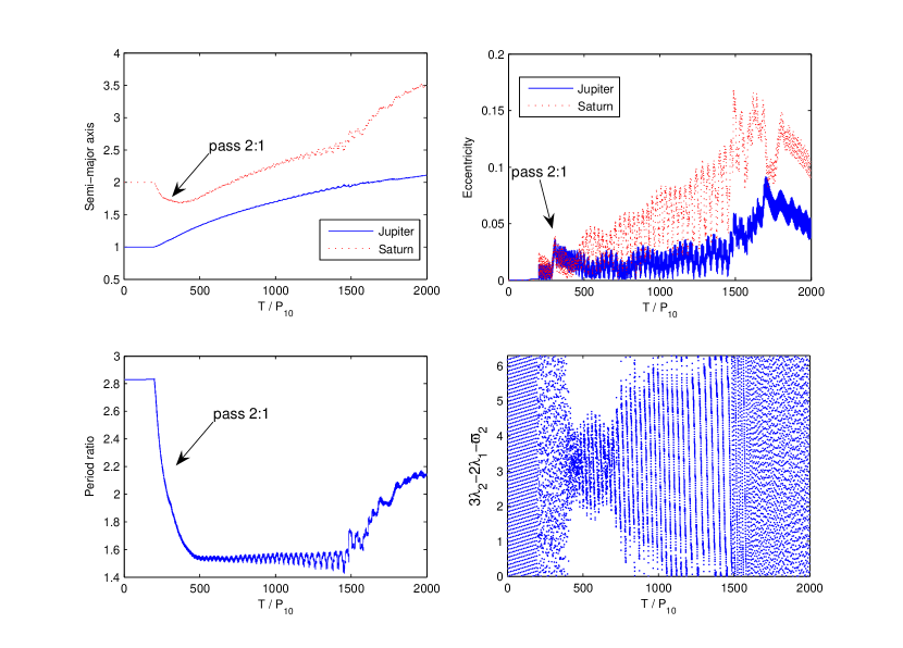
Figure 13: Orbital evolutions of Jupiter and Saturn embedded in a disk where $\sigma=\sigma_{0}r^{-3/2}$. Saturn passes through the position of $2:1$ MMR of Jupiter and then is catched by the $3:2$ MMR. Scattering happens at $T=1500P_{10}$ when $e_{s}\geq 0.15$. (a) Evolutions of the semi-major axes of the two planets. Migration of Saturn becomes unstable after it is trapped into resonance with Jupiter. (b) Evolutions of the eccentricities of the planets. The excitation of Jupiter’s eccentricity by the $3:2$ MMR is behind that of Saturn. (c) Evolutions of the period ratio $P_{S}/P_{J}=(a_{2}/a_{1})^{3/2}$. (d) Evolutions of the resonance angle $\theta\lambda_{2}-2\lambda_{1}-\varpi_{2}$ of $3:2$ MMR. The resonance becomes unstable as the eccentricities keep growing. (A color version of this figure is available in the online journal.)

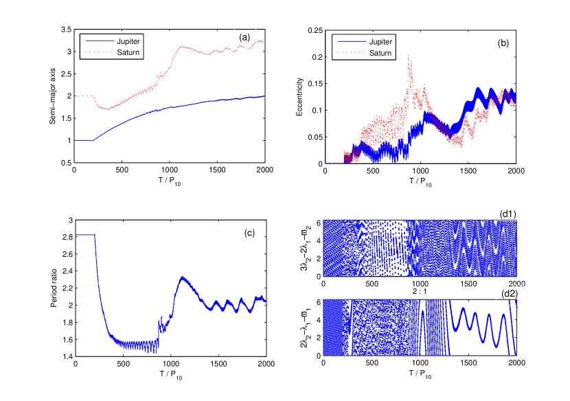
Figure 14: Orbital evolutions of Jupiter and Saturn embedded in a disk where $\sigma=\sigma_{0}r^{-5/3}$. Saturn passes through the position of $2:1$ MMR of Jupiter and then is catched by the $3:2$ MMR. Scattering happens at $T=800P_{10}$ when $e_{s}\geq 0.15$. Eccentricities decrease rapidly after the break of resonance and then the Saturn is trapped by the $2:1$ MMR of the Jupiter at $T=1400P_{10}$ . (a) Evolutions of the semi-major axes of the two planets. (b) Evolutions of the eccentricities of the planets. It clearly shows that the excitation of Jupiter’s eccentricity is previous than that of Saturn in $2:1$ MMR and is laggard in $3:2$ MMR. (c) Evolutions of the period ratio $P_{S}/P_{J}=(a_{2}/a_{1})^{3/2}$. One can see the re-capture of $2:1$ MMR. (d1) and (d2) Evolutions of the resonance angle: $\theta=3\lambda_{2}-2\lambda_{1}-\varpi_{2}$ of $3:2$ MMR(d1) and $\theta=2\lambda_{2}-\lambda_{1}-\varpi_{1}$ of $2:1$ MMR(d2). (A color version of this figure is available in the online journal.)

Second, The two planets may be trapped into different MMRs when the surface density slope $\alpha$ varies. The phenomenon that different types of MMRs that can be trapped during convergent migration depends on the migration speed is revealed in Papaloizou & Szuszkiewicz (2005). In our cases, when the convergent migration is relatively slow, i.e., $\alpha\leq 1$, Saturn is trapped by the $(p+1):p=2:1$ MMR of Jupiter(Figure 10,12). While Figure 13 shows the results with a steeper disk where $\alpha=3/2$. The Saturn passes through the $2:1$ MMR and is trapped by the $3:2$ MMR of the Jupiter. Large $p$ would be achieved by increasing the slope of disk profile ($\alpha$), so that the speed of convergent migration is increased. However, we do not observe any resonances with $p>2$ in our simulations—$p=2$ is the highest value in our results. In fact, a transition from $3:2$ MMR to $2:1$ MMR is observed when the surface density of disk is very steep($\alpha=5/3$), see Figure 14. In this simulation, Saturn first passes through the position of $2:1$ MMR with Jupiter under fast inward migration and is then locked into the $3:2$ MMR with Jupiter. When the resonance established, the two planets migrate outward together, and at the mean time the migration of Saturn becomes unstable as its eccentricity keeps growing. After several hundred orbits, when the eccentricity of Saturn grows to $e>0.15$, the $3:2$ MMR breaks and Saturn is scattered outward. As soon as the resonance breaks, eccentricities of both the two planets are damped effectively by the gas disk and then Saturn is captured by the $2:1$ MMR of Jupiter. This result is consistent with that of Pierens & Nelson (2008), and we find the MMR is not so stable for high eccentricities of planets when they are embedded in a steep disk($\alpha>1$).

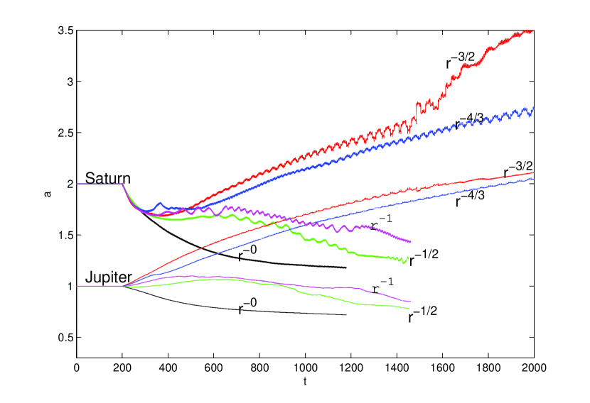
Figure 15: Migrations of Jupiter and Saturn embedded in different disk where the density slope $\alpha$ varies from $0$ to $3/2$. The two planets migrate inward when $\alpha<\frac{1}{2}$, and migrate outward when $\alpha>1$. It shows a transitional state when $\frac{1}{2}<\alpha<1$. (A color version of this figure is available in the online journal.)

Third, the common migration speed and direction of the planet pair in MMR varies with $\alpha$. The speed of common inward migration of the planet pair slows down as $\alpha$ increases. When $\alpha>1$, the two planets reverse their migration to outward, and the migration speed increases as $\alpha$ increases, see Figure 15. This phenomenon can be understood as follows. In the case of one planet, Jupiter undergo type II migration in the viscous disk. Each unit gas ring suffers a viscous torque

$$\Gamma_{\nu}=2\pi r^{2}\nu\sigma\frac{rd\Omega}{dr},$$ (15)

where $\nu$ is the viscosity, $\sigma=\sigma_{0}r^{-\alpha}$ is the surface density of gas disk, $\Omega\sim r^{-3/2}$ is the angular velocity of Kerplerian motion. Assuming a constant $\nu$ across the disk, the viscous torque $\Gamma_{\nu}=-3\pi\nu\sigma_{0}r^{1/2-\alpha}$. By further assuming the disk remains Kelperian flow and integrating the motion equation in the azimuthal direciton, the angular momentum transportation per unit mass is governed by following formula:

$$\dot{r}\frac{d(r^{2}\Omega)}{dr}=\frac{1}{2\pi r\sigma}\frac{\partial\Gamma_{\nu}}{\partial r}+\Lambda,$$ (16)

where $\Lambda$ denotes the local injection rate of angular momentum per unit mass into the disk gas from the planet(Lin & Papaloizou, 1986). The effect of $\Lambda$ vanishes when the planet is treated as a part of the disk in type II migration. Then we can obtain the radial movement of the gas under the effect of viscous torque:

$$\dot{r}=\frac{1}{2\pi r\sigma}\frac{\partial\Gamma_{\nu}/\partial r}{d(r^{2}\Omega)/dr}=-3\nu(\frac{1}{2}-\alpha)r^{-1}.$$ (17)

Since Jupiter now follows the movement of the gas, this in fact results in an inward(or outward) migration of the planet at $\alpha<1/2$ ( $\alpha>1/2$, respectively). It can be seen from Panels (a1) and (b1) in Figure 12, the initial stage ($t=200-500P_{10}$) of Jupiter evolution (before it meets Saturn).

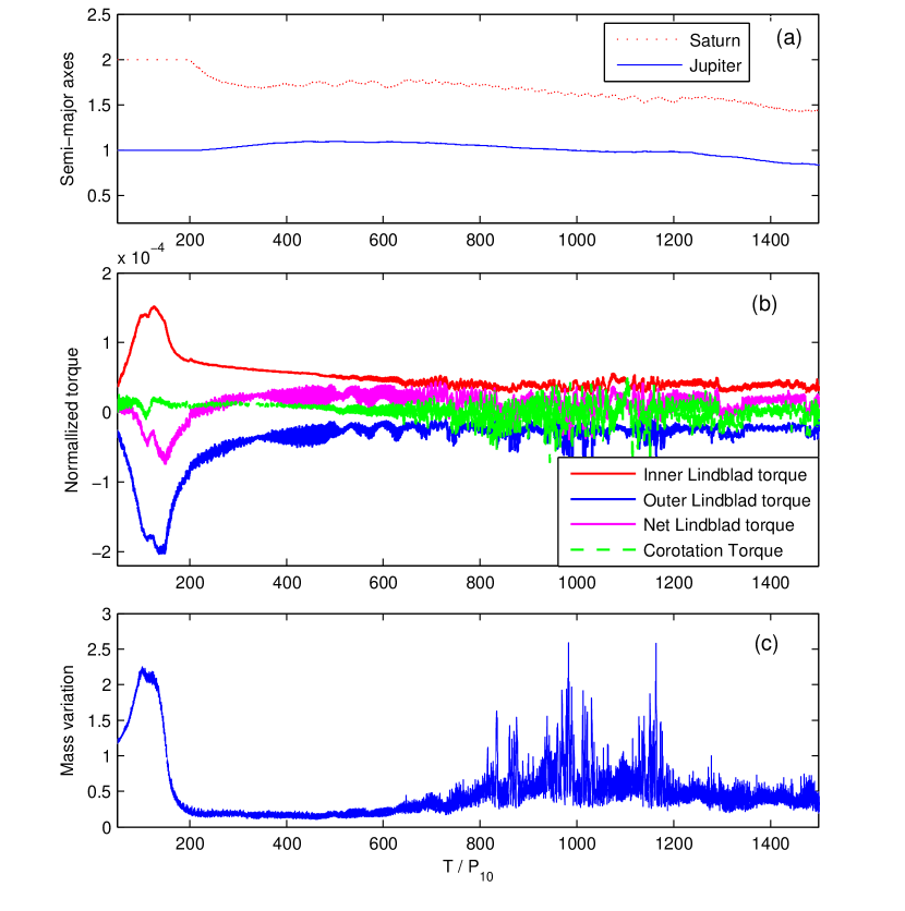
Figure 16: (a) Evolutions of the semi-major axes of Jupiter and Saturn. (b) Evolutions of the inner, outer and net Lindblad torques as well as the corotation torque exerted on Jupiter. The net Lindblad torque is positive at the release moment ($t=200P_{10}$), then a negative corotation torque rises and dominates Jupiter’s migration($t>700P_{10}$). (c) Mass variation within the coorbital zone of Jupiter. The large oscillations after $t=700P_{10}$ result in the negative corotation torque which reverse the migration of Jupiter. The surface density profile is $\sigma=\sigma_{0}r^{-1}$ in this simulation. (A color version of this figure is available in the online journal.)

The presence of Saturn complicates the situation. Since Jupiter is massive than Saturn, Saturn is in fact forced to migrate with Jupiter when $\alpha>4/3$(Figure 13 and 14). In the case of $1/2<\alpha<1$, our simulation shows that the presence of Saturn perturbs the previous outward migration of Jupiter, and makes it undergo slight inward migration(see Figure 12). The reason is that when Jupiter encounters Saturn which is under fast inward migration, its outward migration is slowed down. Then, the eccentricity of Jupiter is excited by the $2:1$ MMR. As the orbit becomes eccentric, Jupiter cuts into the inner part of the gas disk and this causes a negative corotation torque. Figure 16 shows the evolution of the torques exert on Jupiter and the mass variation within the coorbital zone of it. It clearly shows that, after $t=700P_{10}$, the large mass variation results in a negative corotation torque that reverses the migration of Jupiter. The moment $t=700P_{10}$, is just the moment that the eccentricity of Jupiter exceeds $0.17$ which is the critical value required by Jupiter to cut into the inner gas disk (obtained by set $ae>2.5R_{Hill}$, with $R_{Hill}$ the Hill radius of Jupiter).

In this section we show that, for Jupiter and Saturn embedded in a gaseous disk, their convergent migration rate, type of MMRs and subsequent common migration depend on the density slope $\alpha$ of the gas disk. The direct reason for these effects is the different torques(direction, value and type) exert on the planets, which vary with $\alpha$.

3.2 Torque analysis

To understand the phenomena shown in previous section more deeply, we present here some torque analysis based on the linear estimation. After the release of planet at $t=200P_{10}$, the migration of Jupiter couples with the response of gas disk. Since the coorbital zone of Jupiter is effectively cleared, the angular momentum transportation between the inner and outer disk are mainly done by the Lindblad torques. Due to the lack of Lindblad torques expression for a disk under the perturbation of Jupiter, we estimate the differential torque from linear estimation. The $m$th-order Lindblad torque can be expressed as(Ward, 1997; Papaloizou & Terquem, 2006):

$$\Gamma^{LR}_{m}=\frac{{\rm sign}(\Omega_{p}-\Omega)\pi^{2}\sigma(r)}{3\Omega_{p}\Omega\sqrt{1+\xi^{2}}(1+4\xi^{2})}\Psi^{2},$$ (18)

where $\Omega,\Omega_{p}$ are the angular velocity at the specific location of Lindblad resonance and the planets, respectively. $\xi$ is a function that ensures the cutoff of the Lindblad torques at large $m$. This is naturally satisfied when the density vanishes in the gap around the planet. $\Psi$ is the force function which reads:

$$\Psi=r\frac{d\psi_{m}}{dr}+\frac{2m^{2}(\Omega-\Omega_{p})}{\Omega}\psi_{m}.$$ (19)

By a high order interpolation and averaging along azimuthal direction, we obtain the numerical density $\sigma(r)$ and angular velocity $\Omega(r)$ distribution in the disk at certain time. Then we determine the resonance positions for each $m\leq 80$ as well as the Lindblad torque rises there through Equations (18) and (19).

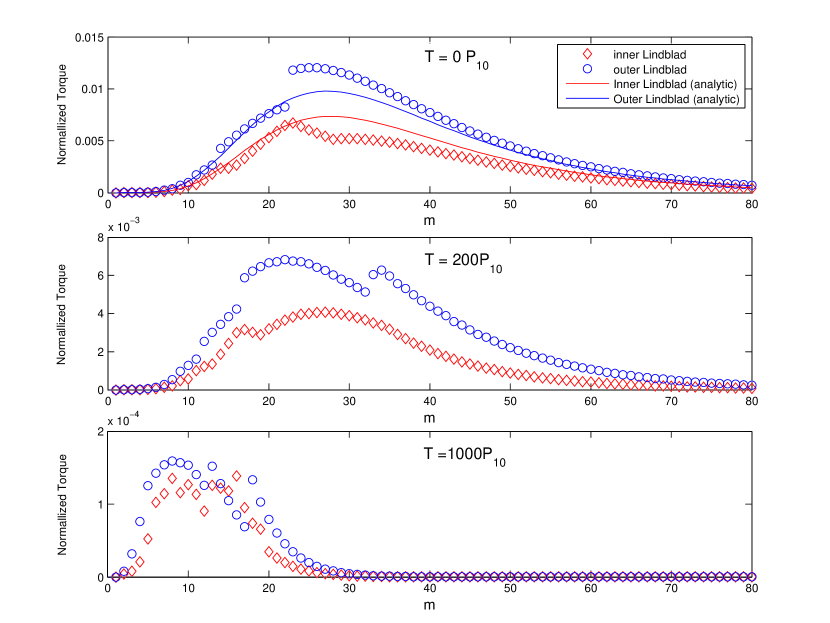
Figure 17: The $m$-th inner and outer Lindblad torques exerted on Jupiter at different times, where $|m|=2-80$. The density profile of the disk in which the two planets embedded is $\sigma=\sigma_{0}r^{0}$. From the top to the bottom, the time points are the initial moment, the release moment and the moment after common gap has formed, respectively. At initial moment, the torques are calculated as if Jupiter was embedded in an unperturbed disk. The solid lines denote the analytic results while the diamonds and circles denote the semi-analytic results. Note that the outer Lindblad torque is always larger than the inner one and the position of maximum value moves left as the gap becomes deeper and wider. The kinks in the numerical results indicate the sudden changes of density or angular velocity distribution of gas, or the failures of locating the exact positions of resonances( extrapolation value is adopted instead), which is mainly due to the lack of radial resolution of the numerical data.

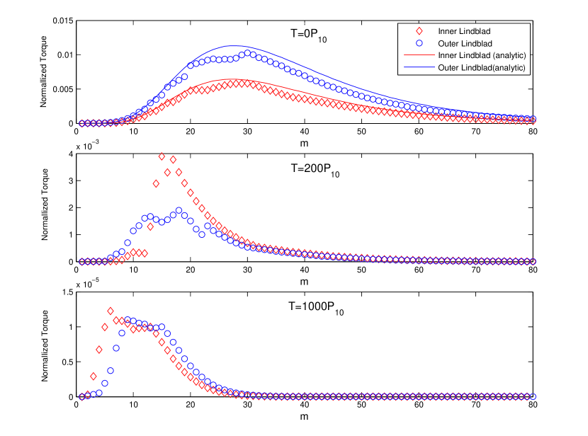
Figure 18: The $m$-th($|m|=2-80$) inner and outer Lindblad torques exerted on Jupiter which embedded in a disk where $\sigma=\sigma_{0}r^{-3/2}$. From the top to the bottom, the time points are the initial moment, the release moment and the moment after common gap has formed, respectively. At initial moment, the torques are calculated as if Jupiter was embedded in an unperturbed disk. The solid lines denote the analytic results while the diamonds and circles denote the semi-analytic results. Note that the inner Lindblad torque becomes larger than the outer one at the release moment. Compared to Figure 17, one may find that the inner Lindblad torque almost remains the same level while the outer one decreases a lot. This could be explained by the mass reduction in the outer disk caused by Saturn.

In a flat disk, we find that the result follows the analytic prediction that the outer Lindblad torque is always stronger, see Figure 17. However, the existence of Saturn weakens the outer Lindblad torques exerted on Jupiter by pushing gas outward away. And the inner disk is strengthened by the steep density profile when $\alpha>0$. Figure 18 shows the differential Lindblad torque exerted on Jupiter at the beginning of simulation ($t=0$), the moment of release ($t=200P_{10}$) and the moment when the common gap has well formed ($1000P_{10}$), in a disk where $\alpha=3/2$. At the beginning of simulation, when the disk is still unperturbed, the numerical results are fit well with the analytic results except at $25\leq m\leq 40$. With the time passing by, both of the inner and outer torques decrease and the position of maximum moves toward smaller $m$, which corresponds to the gap formation process. At the release moment, when the Saturn has already formed, the outer torque decreases more than the inner one does, thus the net torque changes to positive. This positive torque drives Jupiter to migrate outward. When the gaps of the two planets overlapped, the inner and outer torques of Jupiter become comparable and are much smaller than the initial value by an order of $2-3$. Then, Jupiter is in type II migration effectively.

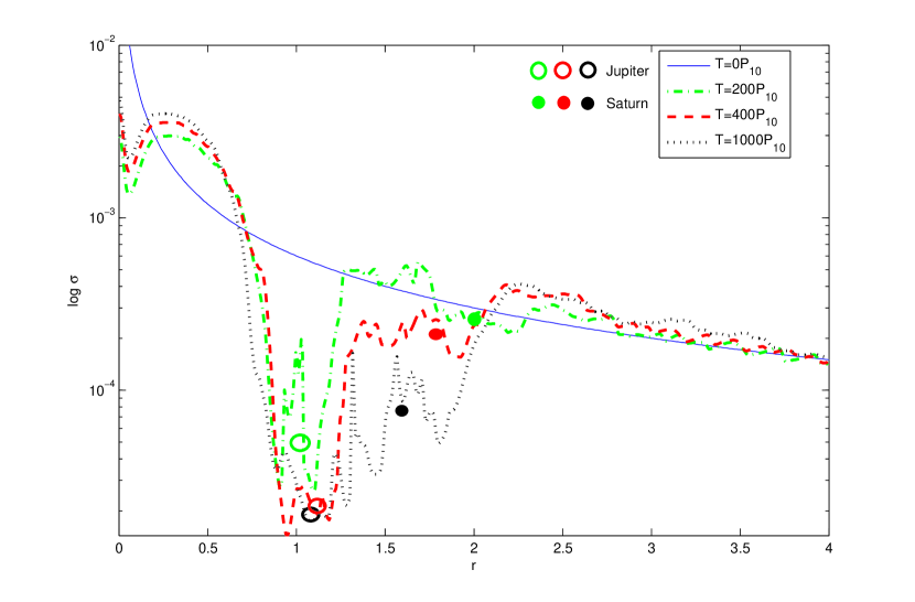
Figure 19: This figure show the cross section of surface density at different moments. The initial density profile is $\sigma=\sigma_{0}r^{-1}$. One can see the overlapping process of two gaps. Note that the gap formation of Saturn is much delayed($T\approx 1000P_{10}$)and the variation of density is acute at Saturn’s vicinity. The coordinates of planets in the figure denote their positions (x axis) and the average gas density around them (y axis). (A color version of this figure is available in the online journal.)

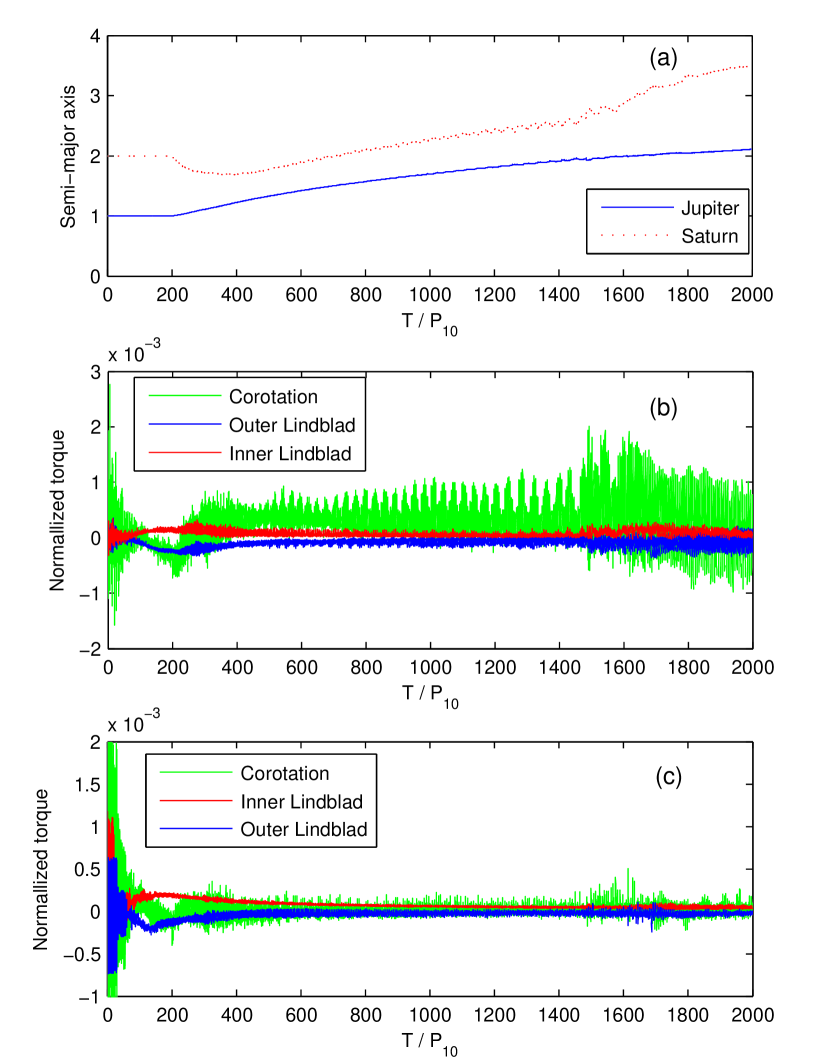
Figure 20: (a) Evolution of the semi-major axes of Jupiter and Saturn. (b) Evolution of the inner/outer Lindblad torques and the corotation torque exerted on Saturn. It shows clearly that the migration of Saturn is dominated by the corotation torque. (c) Evolution of the inner/outer Lindblad torques and the corotation torque exerted on Jupiter. The average value of corotation torque vanishes and the migration of Jupiter is dominated by the Lindblad torques. The surface density profile is $\sigma=\sigma_{0}r^{-3/2}$. (A color version of this figure is available in the online journal.)

However, the migration of Saturn is dominated by the corotation torque. As we have mentioned before, the coorbital zone of Saturn is always perturbed by Jupiter when they are approaching to each other—even after the common gap has formed(Figure 19). The situation is more serious in a steeper disk, because the density profile may amplify the density waves generated by Jupiter. Figure 20 shows the torque evolutions of both Jupiter and Saturn embedded in a gas disk where $\sigma\sim r^{-3/2}$. Although the amplitude of corotation torque is comparable to that of Lindblad torque exerted on the Jupiter, it oscillates around zero and its average effect vanishes. The outer Lindblad torque is weakened by Saturn and the net differential torque is slightly above zero.

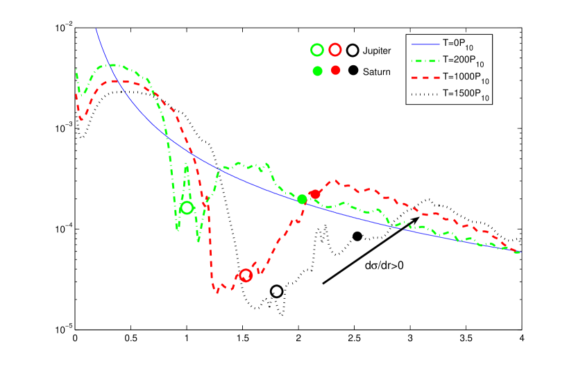
Figure 21: This figure shows the cross section of surface density at different moments. The initial density profile is $\sigma=\sigma_{0}r^{-3/2}$. The common gap forms after $1000P_{10}$ evolution time. One may notice that the density gradient is positive $\frac{d\sigma}{dr}>0$ at the out edge of the common gap, which produces positive corotation torque who drives Saturn outward away. The coordinates of planets in the figure denote their positions ($x$ axis) and the average gas density around them ($y$ axis). (A color version of this figure is available in the online journal.)

At the mean time, the corotation torque exerted on Saturn overwhelms the Lindblad torques. At the moment of release when $T=200P_{10}$, the corotation torque is negative since the density gradient is not perturbed much and still maintain negative around Saturn. Then, as the two planets approaching to each other, the density gradient within the vicinity of Saturn changes to positive and the corotation torque evolves to positive as well. At this moment, Saturn lies close to the outer edge of the common gap, see Figure 21. When $3:2$ MMR is established, the orbit of Saturn becomes more and more eccentric. This makes Saturn cut through the outer edge of the gap periodically, and generates periodical torques. When the eccentricity of Saturn reaches $0.15$, it is scattered outward by the increasing corotation torque and the resonance breaks(Figure 13 and 14).

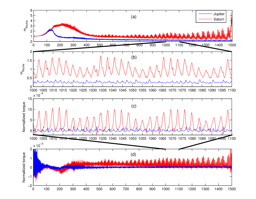
Figure 22: Panel (a) shows the evolution of mass variations within the coorbital zone of Jupiter and Saturn. Panel (b) zooms in from $T=1000P_{10}$ to $T=1100P_{10}$. Panel (c) shows the evolution of corotation torque. Panel (d) zooms in from $T=1000P_{10}$ to $T=1100P_{10}$ too. The initial surface density profile is $\sigma=\sigma_{0}r^{-3/2}$. One may find the oscillations of the mass variation and the corotation torque match well. The short period of oscillations correspond to the orbit period and the long period is the libration period of the horse-shoe orbit, which equals to $32P_{10}$ at the position of Saturn. (A color version of this figure is available in the online journal.)

As shown by Figure 22, the mass variation within the coorbital zone of Saturn and the corotation torques exerts on it are strongly correlated. In the plot, the short period corresponds to the orbit motion of Saturn, as Saturn cuts into the outer disk in every orbit. And the long period is the libration time of Saturn which reads:

$$t_{\rm lib}=\frac{2\pi a}{R_{co}}\left|\frac{1}{2}r\frac{\partial\Omega}{\partial r}\right|^{-1},$$ (20)

where $R_{co}$ is the half width of the coorbital zone and usually equals to $2.5$ times of the Hill radius of Saturn. The libration period at the position of Saturn is $t_{\rm lib}\approx 32P_{10}$, as shown in Figure 22, from $T=1000P_{10}$ to $1100P_{10}$. This is also the period that the coorbital mass exchanges its angular momentum with the planet(Ward, 1991; Masset & Papaloizou, 2003). The mass variations are normalized by the unperturbed coorbital mass of each planet respectively. For Saturn, the peak value immediately before the onset of instability is about 5 times greater than its unperturbed state, which is roughly $10^{-4}$ in our unit, or $30\%$ of the mass of Saturn. The angular momentum exchange between this part of coorbital mass and Saturn results in the corotation torque that dominates Saturn’s migration.

In this section we show that the different migration rates and directions of the two giant planets are the results of the combination of Lindblad and corotation torques, which depend on the density slope of the disk ($\alpha$). The corotation torque exerted on Saturn weakens the stability of Saturn’s orbit. The unstable migration is more serious in the disk with large $\alpha$, see Figure 12-14. And furthermore, the breaks of MMR are observed when $\alpha\geq 3/2$(Figure 13 and 14). To analysis these breaks is helpful to understand the orbital evolution following the convergent migration of Jupiter and Saturn. The details and analysis are presented in the next section.

3.3 Stability of MMRs

MMRs are common results of the convergent migration of Jupiter and Saturn. In this section, we investigate the stability of them. As showed in Table 2, Saturn may be trapped by the $2:1$ MMR of Jupiter when the disk is nearly flat and may reach the $3:2$ MMR if the surface density profile is steep, e.g. $\alpha>1$. Furthermore, the $3:2$ MMR of the Jupiter and Saturn is not stable as their eccentricities keep growing, while the $2:1$ MMR seems to be more robust even at relatively high eccentricities $\sim 0.2$(e.g., Figures 10 and 12).

The instability of planets in the $2:1$ or $3:2$ MMRs could be caused by the overlap of two nearby resonances when the eccentricity is large enough. In the case that both two planets are with equal masses ($m$) and move in circular orbits, the overlap of nearby resonances occurs when the difference of their semi-major axes is smaller than a limit(Wisdom, 1980; Gladman, 1993),

$$\frac{\Delta a}{a}\sim\frac{2}{3p}<2(\frac{m}{M_{*}})^{2/7},$$ (21)

where the relationship of $n_{1}/n_{2}=(p+1)/p=[(a+\Delta a)/a]^{3/2}\approx 1+3/2(\Delta a/a)$ is used, with $n_{1},n_{2}$ the mean motion of the two planets. Assuming $m/M_{*}=(0.27-0.95)\times 10^{-3}$ for Jupiter and Saturn, the application of Equation (21) give $p>p_{\rm min}\sim 3-4$ for the overlap between $(p+1):p$ and $(p+2):(p+1)$ MMRs.

However, when $p\leq p_{min}$ their MMRs can also overlap if they are in high eccentric orbits. In the framework of restricted three-body problem, a planetesimal embedded in a gas disk will be trapped into the outer resonance of a massive body. Kary et al. (1993) estimate of the minimum separation between MMRs below which the planetesimals may undergo chaotic instability due to the MMR overlap:

$$\frac{\Delta a}{a}\sim[(\frac{8\pi m_{p}}{3M_{*}})^{2}(\frac{3v_{\rm dif}}{2v_{\rm kep}})]^{1/9},$$ (22)

where $m_{p}$ refers to the mass of planet and $e$ is the orbital eccentricity of planetesimal, $v_{\rm dif}$ is the difference between the gas velocity and the local circular Keplerian velocity $v_{\rm kep}$. This velocity difference is a result of the pressure rose by the slope of the surface density $\alpha$ in the disk, which makes the gas circle the central star at a sub-Keplerian velocity, and is referred as the drag effect of the gas disk. In a nearly flat disk, $v_{\rm dif}/v_{\rm kep}$ is usually tiny, for example, $v_{\rm dif}/v_{\rm kep}=0.002$ at $r=1$ when $\sigma\sim e^{-r^{2}/53}$, while it increases to $\sim 0.01$ when $\alpha>3/2$. Use the approximation that $3/2(\Delta a/a)\approx 1/p\sim 1/(p+1)$ and the relation obtained by Weidenschilling & Davis (1985):

$$e\approx(\frac{v_{\rm dif}/v_{\rm kep}}{p+1})^{1/2},$$ (23)

we can get the minimum eccentricity, above which the $(p+1):p$ and $(p+2):(p+1)$ MMRs will cross, from Equation (22):

$$e_{min}\sim\frac{3M_{*}}{8\pi m_{p}}(\frac{2}{3}\frac{1}{p+1})^{5}.$$ (24)

This gives $e_{min}\approx 0.065$ for $p+1:p=3:2$ MMR, and $\approx 0.49$ for 2:1 for a Jupiter mass disturber. Although Equation (24) is obtained from the restrictive three-body problem, our simulation show that it also applies to Jupiter-Saturn case. In fact, we find the $3:2$ MMR breaks as soon as the eccentricity of Saturn reaches $0.15$ and larger $\alpha$ doesn’t change this value but only makes instability happen earlier, see Figure 13 and 14. The $2:1$ MMR is much more robust, because it only requires $e\leq 0.5$ to maintain stable and the eccentricity excited by $2:1$ always stay at $e\leq 0.2$, see Figures 10 and 12.

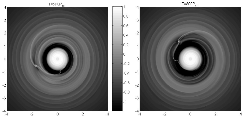
Figure 23: Density contours at $T=500P_{10}$ and $T=800P_{10}$ in a disk where $\sigma=\sigma_{0}r^{-3/2}$. One may find the Jupiter has opened a clear gap while the Saturn is still surrounded by gas at $T=500P_{10}$ (left figure). And the shock waves generated by Jupiter perturbs the coorbital zone of Saturn when the two gaps are overlapping $T=800P_{10}$ (right figure).

The other reason for the instability of MMR is the runaway migration induced by the corotation torque. We had shown that, a moderate planet will undergo runaway migration(Type III migration) when its coorbital zone is perturbed heavily by the density waves generated by the other giant planet(Zhang et al., 2008; Zhang & Zhou, 2008). It is believed that two giant planets would be trapped and migrate together when their gaps overlapped well. It’s true that when the density distribution of disk is nearly flat, the convergent migration is relatively slow and Saturn has enough time to clean its coorbital zone before it interacts with Jupiter directly. However, when the disk is steep, say $\sigma\sim r^{-3/2}$, the convergent migration is so fast that the Jupiter would catch Saturn to the $3:2$ MMR before the later one opens a clean gap, see Figure 23. At this time, Saturn is forced to migrate with Jupiter while the corotation torque still dominates its migration. As we can see from Figure 13, the migration curve becomes very oscillatory as soon as Saturn is trapped by the MMR with Jupiter.

In fact, eccentricity plays an essential role on triggering runaway migration even if a clean gap formed around the planet orbit. As we mentioned in previous section, as soon as the giant planet undergoes eccentric motion, it cuts through the edge of the gap periodically when $ae\geq R_{\rm gap}$, where $R_{\rm gap}$ is the width of the gap. Then, a periodic torque rises as a result of the replenishment of gas into the vicinity of the planet. This torque may change the direction of planet’s migration (see Figure 16) or kick the planet away quickly. A good approximation for the gap width is $R_{\rm gap}\approx 2.5R_{\rm Hill}$, the same with the radius of the coorbital zone of a giant planet by assuming the viscosity is low, where $R_{\rm Hill}$ is the Hill radius of this planet. In the case of Saturn, it requires $e\sim 0.15$ to allow Saturn cut into the disk. However, as Saturn lies outside the orbit of Jupiter, it can only touch the outer edge of the common gap, where the surface density gradient is positive and the corotation torque exerted on it is positive as well, see Figure 21. Thus, Saturn tends to be scattered outward at this kind of configuration.

According to our results and analysis, we find that the instability of MMR is mainly due to the large eccentricity excited by the MMR itself. High eccentricity either leads to the overlap of MMRs or makes the planet cut into the disk and generates strong corotation torque. As the eccentricity evolutions of the two planets locked in resonance vary with the type of resonance(Michtchenko et al., 2006), density slope ($\alpha$) will affect the final orbit configuration of the planet pair.

4 Conclusions and discussions

A series of high resolution hydrodynamic simulations have been performed to investigate the orbital evolution of Jupiter and Saturn embedded in a protostellar disk. We focus on the effects of different surface density profiles of the gas disk where $\sigma\propto r^{-\alpha}$. The instability of mean motion resonance caused by the convergent migration is also studied. According to the results and analysis of our simulation, we summarize our conclusions as follows, as well as the discussions and implications for these results.

(1) The existence of Jupiter(massive planet) delays the gap formation process of Saturn(light planet) and generates great perturbations within the coorbital zone of Saturn. These perturbations result in the inward or outward runaway migration(type III migration) of Saturn, depending on $\alpha$, the density slope of the gas disk.

The effects of the pre-formed giants are very important for understanding the orbital evolution of a multiple planet system. To investigate these effects, we fix the very first $200P_{10}$ orbits of both the two planets when they are growing from $0.1$ Earth mass to 1 Jupiter and 1 Saturn mass respectively, then we release them at the same time. This, in fact, assumes that the Jupiter had formed before the Saturn did since the gap of Jupiter had well formed while the Saturn’s hadn’t yet.

The orbital evolutions of the planets form later are greatly affected by the pre-formed giant ones. The first generation of giant planets strongly modified their neighborhood by opening gaps at several Hill radius from themselves (Bryden et al., 2000), as well as the planetesimal gaps (Zhou & Lin, 2007). Pierens & Nelson (2008) had shown that the light planets will be trapped at the edge of the giant planet’s gap. This halt is because of the balance between the Lindblad torque and the corotation torque which rises at the density jump. This happens when the mass of the outer planet is low: $m_{2}\leq 20M_{\oplus}$. For massive outer planets,i.e., $m_{2}\sim M_{J}$, the strong tidal effect guarantees the gap formation process and slow type II migration could be expected. The situation becomes complex when the outer planet has a moderate mass, $m_{2}\sim M_{S}$ which is critical to open a gap. Its orbital evolution thus strongly depends on the initial conditions, for example, the initial density profile of the disk $\alpha$.

Zhang et al. (2008) had shown that the existence of the gaseous disk expands the interaction region of the proto-planets. As we have shown in the previous section, the tidal effect of Jupiter keeps pushing the gas away from its coorbital zone and replenish the gap of Saturn (see Figure 19 and 21). This effect increases as $\alpha$ increases(Figure 11) and drives the orbital evolution of the system unstable. If the initial separation is large or the disk is nearly flat, clear gaps would form around the planets’ orbit and gentle convergent migration could be expected. This will result in a less compact and more stable system.

(2) The convergent migration rate is proportional to the surface density slope $\alpha$. And, as a result, the types of MMRs depend on $\alpha$ as well. The two planets approach to each other gently when $\alpha<1$, and are locked into $2:1$ MMR. When $\alpha>1$, the convergent migration is fast and the $3:2$ MMR is reached.

The convergent migration rate is one of the most critical issues to determine the consequential migration of the planet pair. Many factors may affect this rate, for example, the masses of the two planets (Pierens & Nelson, 2008), the viscosity and the disk aspect ratio (Morbidelli & Crida, 2007). However, the essential factor which results in differential migration is the various torques by which the planets are driven. These torques intensively relate to the surface density of the disk in which the planets embedded. For a low mass planet, the differential Lindblad torque is negative and the value is proportional to the density slope $\alpha$($\sigma\sim r^{-\alpha}$)(Ward, 1991). The migration of massive planet is determined by the global distribution of the angular momentum(relates to $\alpha$) and the viscosity of the gaseous disk. The corotation torque relates to the vortensity gradient(relates to $\alpha$ as well) within the coorbital zone of planet(Masset & Papaloizou, 2003). The analysis of torques by a semi-analytical method have been shown in the previous section, see Figure 16-18 and 20.

To get the different convergent rate naturally, we choose a series of density profiles of the disk where $\sigma\sim r^{-\alpha}$. Most of the typical density profiles have been adopted, see Table 2. Our results show that the convergent migration rate increases as $\alpha$ increases, see Figure 11. This is reasonable since the migration of Saturn is accelerated by the steep density slope while the migration of Jupiter turns outward when $\alpha>1/2$. The type of resonance is determined by how close the two planets could approach. When the disk is nearly flat, where $\alpha<1$, the $2:1$ MMR is a robust outcome. While the $3:2$ MMR is more favorite in the steep disk where $\alpha>1$. The disk with a density profile around $\alpha\approx 1$ shows a transition phenomena and the high eccentricity of Jupiter reverses its outward migration to inward, see Figure 12 and 16.

(3) The $3:2$ MMR of the two planets is unstable when the eccentricity of Saturn becomes large enough in a steep disk where $\alpha>3/2$. We estimate that the critical value is $e_{s}\sim 0.15$ with our settings.

The $3:2$ MMR of Jupiter and Saturn is thought to be robust for many settings, but we find that this configuration may breaks down when the eccentricity of Saturn grows too high in a gaseous disk where the surface density gradient is pretty steep $\alpha>3/2$. In fact, the eccentricities will be exited as soon as the resonance established no matter the disk is nearly flat or very steep (Figures 10 and 12-14). However, in a steep disk, the situations are different. First, the convergent migration is much faster. This enables the two giant planets get much closer and as a result, the dynamical instability becomes possible, for example, the overlap of resonances. Second, caused by the fast convergent migration as well, the establishment of resonance occurs before a clear common gap formed. This will result in a strong corotation torque which may drive an unstable migration of Saturn, see Figure 13. Third, the steep gradient of density in fact amplifies the density waves propagating from Jupiter to Saturn and results in relatively heavier perturbation in coorbital zone of Saturn.

In our simulations, the planet pair migrates outward when $\alpha>1$. The separation between them increases as they preserve the $3:2$ MMR. Thus, Saturn is pushed outward further and further. At the mean time, the growing eccentricity makes Saturn cut into the outer disk deeper and deeper. The density gradient at the out edge of the common gap is positive and generates positive corotation torque that pushes Saturn outward further. When the eccentricity is high enough, Saturn is scattered outward. Our results show that the critical value is $e\geq 0.15\sim 0.2$ for $3:2$ MMR of Jupiter and Saturn.

We also find that the onset of instability would be suspend when $\alpha$ decreases. In fact, in the case where $\alpha=4/3$, the two planets maintain $3:2$ MMR over $2000P_{10}$, see Figure 15. So the long time stability could also be expected by choosing a proper $\alpha$, and this still needs further simulations. The $2:1$ MMR seems to be more stable for high eccentricities and we find the two planets could be re-locked into $2:1$ MMR just after the break of $3:2$ MMR when they are both migrating outward, see Figure 14.

If the initial density profile of our Solar nebular is relatively steep, e.g. $\alpha>4/3$, then the formation of the main configuration of our Solar system could be this way: (a) Jupiter and Saturn first migrate inward when their masses are still low. (b) By accreting gas from the nearby disk, they grow up quickly. While Jupiter grows much faster than Saturn does through the runaway accretion, and the mass difference results in a convergent migration between them. (c) Then the $3:2$ MMR of Jupiter and Saturn is established and their migration turns outward with the resonance preserved. (d) When the eccentricity of Saturn becomes too high, the resonance breaks down and Saturn is scattered outward to the place near its present location or re-captured by the $2:1$ MMR of Jupiter. Neptune and Uranus are also scattered out away at the mean time. (e) The eccentricities of both the inner rocky planets and the outer gas giant are damped effectively by the gas disk after the instability. (f) After the dissipation of gas, the planets evolve to their present locations by the interaction with the planetesimal disk. Of course, many details are need to be addressed especially for the orbital evolutions of the inner rocky planets. However, compared to the results of Morbidelli et al. (2007), our results suggest that the instability would happens before the dissipation of gas. The remaining gas may corresponds to the low eccentricities of the main planets in our Solar system. And since Jupiter migrates inward before its outward migration, the final location is not far from its birth place.

We also notice that the excitation of Jupiter’s eccentricity is previous than that of Saturn in $2:1$ MMR and is laggard in $3:2$ MMR. Since the eccentricity is a critical issue to guarantee the stability of Jupiter-Saturn pair, its evolution and constraints need to be addressed in details by considering the effect of the interacting disk. The results of a reverse orbital configuration of Saturn and Jupiter is in preparing as well.

5 Acknowledgement

We thank D.N.C. Lin, A.Crida, W. Kley for their constructive conversations. We also thank M. de Val-Borro for providing data for the comparison. Zhou is very grateful for the hospitality of Issac Newton institute during the Program ‘Dynamics of Discs and Planets’. This work is supported by NSFC (Nos. 10925313,10833001,10778603), National Basic Research Program of China(2007CB814800) and Research Fund for the Doctoral Program of Higher Education of China (20090091120025).

Table 1: A short list of extra-solar planets in resonance.

System	No.	$P$ [day]	$M\sin i$ [$M_{J}$]	$a$ [$AU$]	$e$	Refs.
GJ 876	c	30.57	0.56	0.13	0.2	1
(2:1)	b	60.13	1.89	0.21	0.04
HD 128311	b	458	2.3	1.08	0.23	2
(2:1)	c	918	3.1	1.71	0.22
HD 73526	b	188	2.90	0.66	0.19	3
(2:1)	c	377	2.50	1.05	0.14
HD 82943	b	217.9	1.4	0.74	0.46	4
(2:1)	c	456.6	1.78	1.19	0.36
HD 160691	d	310.55	0.52	0.92	0.067	5
(2:1)	b	643.25	1.68	1.5	0.13
HD 45364	b	227	0.19	0.15	0.17	6
(3:2)	c	343	0.66	0.68	0.09
HD 60532	b	201	3.15	0.76	0.27	7
(3:1)	c	605	7.46	1.58	0.038

Note. — References. (1) Marcy et al. 2001;(2) Vogt et al. 2005; (3) Tinney et al. 2006; (4) Lee et al. 2006; (5) Gozdziewski et al. 2007; (6) Correia et al. 2009; (7) Laskar & Correia 2009.

Table 2: A summary of our simulations.

Case	Configuration	Direction	$\sigma$	Resonance	Instability
1	J-S	inward	$\sigma\sim r^{0}$	$2:1$	no
2	J-S	inward	$\sigma\sim e^{-\frac{r^{2}}{53}}$	$2:1$	no
3	J-S	inward	$\sigma\sim r^{-\frac{1}{2}}$	$2:1$	no
4	J-S	inward	$\sigma\sim r^{-\frac{2}{3}}$	$2:1$	no
5	J-S	inward	$\sigma\sim r^{-1}$	$2:1$	no
6	J-S	outward	$\sigma\sim r^{-\frac{4}{3}}$	$3:2$	no
7	J-S	outward	$\sigma\sim r^{-\frac{3}{2}}$	$3:2$	yes
8	J-S	outward	$\sigma\sim r^{-\frac{5}{3}}$	$3:2$ $\rightarrow$ $2:1$	yes

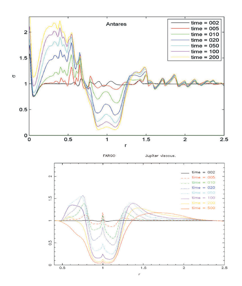
Figure 6: The normalized surface density profiles averaged azimuthally over $2\pi$ after 100 orbits for the viscous simulations. The viscous coefficient $\nu=10^{-5}$. Antares shows the proper behavior of gas under the increasing dissipation effect—the gap becomes narrower and shallower. The results of FARGO are obtained from the web: http://www.astro.su.se/groups/planets/comparison, which is maintained by de Val-Borro.

References

- Bryden et al. (2000) Bryden, G., Róyczka,M., Lin, D. N. C., & Bodenheimer, P. 2000, ApJ, 540, 1091
- Colella (1990) Colella, P. 1990, JCoPh, 87, 171
- Correia et al. (2009) Correia, A. C. M., et al. 2009, A&A, 496, 521
- Crida et al. (2008) Crida, A., Sándor, Z., Kley, W., 2008, A&A, 483, 325
- Gladman (1993) Gladman, B. 1993 Icarus, 106, 247
- Goldreich & Tremaine (1979) Goldreich, P., & Tremaine, S. 1979, ApJ, 233, 857
- Gomes et al. (2005) Gomes, R., Levison, H. F., Tsiganis, K., & Morbidelli, A. 2005, Nature 435, 466
- Gozdziewski et al. (2007) Gozdziewski, K., Maciejewski, A. J., & Migaszewski, C. 2007, ApJ, 657, 546
- Guillot et al. (2006) Guillot, T., & Hueso, R. 2006. MNRAS, 367, L47
- Kary et al. (1993) Kary, D. M., Lissauer, J. J., & Greenzweig, Y. 1993, Icarus, 106, 288
- Kley et al. (2004) Kley, W., Peitz, J., & Bryden, G. 2004, A&A, 414, 735
- Kley et al. (2005) Kley, W., Lee, M. H., Murray, N., & Peale, S. J. 2005, A&A, 437, 727
- Laskar & Correia (2009) Laskar, J., & Correia, A. C. M. 2009, A&A, 496, L5
- Lee et al. (2006) Lee, M. H., Butler, R. P., Fischer, D. A., Marcy, G. W., & Vogt, S. S. 2006, ApJ, 641, 1178
- Lin & Papaloizou (1986) Lin, D. N. C. & Papaloizou, J. C. B. 1986, ApJ, 309, 846
- Lin & Papaloizou (1986) Lin, D. N. C. & Papaloizou, J. C. B. 1986, ApJ, 846, 857
- Marcy et al. (2001) Marcy, G. W., Butler, R. P., Fischer, D., Vogt, S. S., Lissauer, J. J., & Rivera, E. J. 2001, ApJ, 556, 296