Ground-state properties of tubelike flexible polymers

Abstract

In this work we investigate structural properties of native states of a simple model for short flexible homopolymers, where the steric influence of monomeric side chains is effectively introduced by a thickness constraint. This geometric constraint is implemented through the concept of the global radius of curvature and affects the conformational topology of ground-state structures. A systematic analysis allows for a thickness-dependent classification of the dominant ground-state topologies. It turns out that helical structures, strands, rings, and coils are natural, intrinsic geometries of such tubelike objects.
PACS: 05.10.-a: Computational methods in statistical physics and nonlinear dynamics; 87.15.A-: Theory, modeling, and computer simulation; 87.15.Cc: Folding: thermodynamics, statistical mechanics, models, and pathways

1 Introduction

The structural properties of macromolecules composed of covalently bound atomic complexes are of major interest as the functionality of these molecules, e.g., biopolymers, strongly depends on the formation of stable ground-state conformations with several substructures. One can resolve these structures by means of several experimental techniques like molecular microscopy, NMR or X-ray analyses.

As these techniques are relatively costly and can often hardly be generalized, the structural behavior of polymers and its modeling got into the focus of computer simulations, too. In early approaches, polymers were modeled as topologically one-dimensional strongly coarse-grained bead-spring systems, which were treated by means of Monte Carlo and molecular dynamics computer simulations [1, 2, 3]. Later, all-atom peptide simulations were performed with the intention to study real biopolymers, in particular their native states and the folding pathway to native states [4, 5]. As this is still a great challenge and moreover restricted to comparatively short objects, the interest in the earlier simple models continues until today. There is still a great variety of one-dimensional stringlike models of flexible polymers under current investigation (see, e.g. [6, 7, 8, 9]).

Biopolymers do have side chains, however, which are responsible for the variety of forms and functions. As these side chains involve strict steric constraints for the structure of the polymer, the central question is therefore: What degree of abstraction (coarse-graining) is reasonable to treat certain features of real (bio)polymers or, the other way around, which features can we reliably study with a certain degree of abstraction? One can, for example, understand certain universal properties of the well-known coil-globule transition by studying the simplest stringlike models [10, 11], whereas the formation of secondary structures will generally not be answered satisfactorily.

We are going to approach this problem in the present work by studying in detail some kind of “intermediate” model. It is derived from a linelike model where additionally the steric influence of monomeric side chains in real biopolymers will be effectively introduced, without taking into account further microscopical details, by a geometric thickness constraint, extending the model to a three-dimensional tube [16, 17, 18]. An elegant possibility to implement the thickness constraint is provided by the concept of the global radius of curvature which “provides a concise characterization of the thickness of a curve” [19]. We will see, that we already get quite interesting qualitative and quantitative answers to the question of secondary structure formation under these conditions.

The structure of this paper is as follows: In Sect. 2.1 we first introduce the model we use and shortly describe our methods, and in Sect. 2.2 we explain in more detail, how the thickness is implemented in our model. After introducing briefly some observables in Sect. 3.1, we study in Sect. 3.2 the ground states of the model in great detail, depending on the thickness with inter-monomer interaction parameters kept fixed. Furthermore, in Sect. 3.3 we look at special problems like crystallization into regular lattice structures and the appearance of biologically relevant structures depending on a variable interaction length scale. The paper concludes in Sect. 4 with a summary of our main findings.

2 Technical details

2.1 Model and Methods

To model flexible homopolymers we use a thick, tubelike off-lattice chain with fixed bond length and pure Lennard–Jones (LJ) interaction between all, except for the neighboring, monomers:

$$V_{\mathrm{LJ}}(r_{ij})=4\left(\left(\frac{\sigma}{r_{ij}}\right)^{12}-\left(\frac{\sigma}{r_{ij}}\right)^{6}\right)\,,$$ (1)

where $r_{ij}=|\mathbf{x}_{i}-\mathbf{x}_{j}|$ is the distance between two monomers at positions $\mathbf{x}_{i}$ and $\mathbf{x}_{j}$. Note that $V_{\mathrm{LJ}}(r_{ij})=0$ for $r_{ij}=\sigma$ and that the potential minimum $V_{\mathrm{LJ}}(r_{ij})=-1$ is located at $r_{ij}^{\rm min}=2^{1/6}\,\sigma$. The bond length $r_{i,i+1}$ is set to $1$.

We investigate the model by means of Monte Carlo computer simulations and numerical methods. For the ground-state search, one may use for example the multicanonical method [23, 24, 25], the efficient random walk algorithm introduced by Wang and Landau [26, 27] or parallel tempering [28, 29]. For this purpose, all methods work nearly equally well as one does not have to care about the quality of the sampling of the whole configuration space and the performance depends mainly on the parameters of the methods. Additionally, we use standard conjugate gradient methods to refine the results [30]. For the methodologically more challenging task of studying the thermodynamic behavior [31, 32], we use the multicanonical method, calculating the multicanonical weights with the help of the Wang–Landau algorithm [25]. Chains with different thicknesses have always been simulated independently from each other, not at least to avoid uncontrollable correlations.

2.2 Thickness and Global Radius of Curvature

What precisely motivates us to simulate coarse-grained homopolymer models with geometric constraints like “thickness”? And, how is this realized in the model? Polymers in biology are not thin strings. Amino acids, and thus proteins, do have rather extended side chains sterically avoiding each other. It might therefore be useful to introduce a constraint that mimics this volume exclusion. Furthermore, it has been shown [33] that tube models for polymers allow for the formation of stable regions of biologically relevant (sub)structures like helices or sheets, in contrast to simpler linelike polymer models [34]. In addition, the introduction of such a geometric constraint restricting the conformational space might even lead to some technical advantages for finding minimal energy conformations in sophisticated stochastic ground-state searches [32].

To define the self-avoiding tube, we use the concept of the global radius of curvature $r_{\mathrm{gc}}$, which is a concise characterization of the thickness of a curve [19, 34]. The global radius of curvature is defined as the minimal radius of all circumcircles $r_{\mathrm{c}}$ of any three monomers in the chain:

$$r_{\mathrm{gc}}(\mathbf{X}):=\min\{r_{\mathrm{c}}(\mathbf{x}_{i},\mathbf{x}_{j},\mathbf{x}_{k}),\,\forall\,1\leq i<j<k\leq N\}\,.$$ (2)

The circumradius $r_{\mathrm{c}}$, i.e., the radius of curvature, of three points located at positions $\mathbf{x}_{i}$, $\mathbf{x}_{j}$ and $\mathbf{x}_{k}$ can be calculated as

$$r_{\mathrm{c}}(\mathbf{x}_{i},\mathbf{x}_{j},\mathbf{x}_{k})=\frac{r_{ij}\,r_{ik}\,r_{jk}}{4A_{\Delta}(\mathbf{x}_{i},\mathbf{x}_{j},\mathbf{x}_{k})}\,,$$ (3)

where $A_{\Delta}(\mathbf{x}_{i},\mathbf{x}_{j},\mathbf{x}_{k})$ is the area of the triangle spanned by the three points at $\mathbf{x}_{i}$, $\mathbf{x}_{j}$ and $\mathbf{x}_{k}$. Note, that the model uses a three-point interaction between monomers, in contrast to two-point interactions typically used in hard-sphere models to incorporate volume exclusion effects. Given a polymer conformation $\mathbf{X}=(\mathbf{x}_{1},\dots,\mathbf{x}_{N})$ with $N$ monomers, we then define as its thickness $d$ twice the global radius of curvature $r_{\mathrm{gc}}(\mathbf{X})$: $d(\mathbf{X})=2r_{\mathrm{gc}}(\mathbf{X})$.

The other way around, given a thickness constraint $\rho$ such that $d\geq 2\rho$, one can construct an excluded volume depending on $\rho$ around two monomers, which is “forbidden” for any other monomer. A polymer conformation then complies with the thickness constraint if any other monomer resides outside these circles. The partition function reads in this case:

$$Z_{\rho}=\int\mathcal{D}X\Theta(r_{\mathrm{gc}}(\mathbf{X})-\rho)\,\mathrm{e}^{-E(\mathbf{X})/{T}}\,,$$ (4)

where $\Theta(z)$ is the Heaviside function and

$$E(\mathbf{X})=\sum_{i,j>i+1}V_{\mathrm{LJ}}(r_{ij})$$ (5)

is the energy of the conformation $\mathbf{X}$.

Intuitive illustrations of this approach can be found in [18], where it has been chosen for the analysis of ringlike tube polymers. It is used as well in [31, 32] where the pseudophases of secondary structures for tubelike polymers are investigated. As a remark: Even though some universal properties (such as, e.g., critical exponents) do not depend on the exact definition of the thickness, the model may behave differently by imposing the hard constraint $d=2\rho$, i.e., by replacing $\Theta(r_{\mathrm{gc}}(\mathbf{X})-\rho)$ with $\delta(r_{\mathrm{gc}}(\mathbf{X})-\rho)$ in the partition function (4) [18].

3 Results and Discussion

In the following, we first analyze in detail the ground states and ground-state regions of tubelike polymers for chain lengths $8\leq N\leq 13$ with Lennard–Jones parameter $\sigma=1$, where $V_{\mathrm{LJ}}=0$ for covalently bound monomers. Furthermore, we investigate the influence of the tube thickness in connection with the length scale $\sigma$ of the nonbonded LJ interaction on the formation of different classes of structures. In this analysis, particular emphasis will be dedicated to secondary structures such as helices and strands, being most relevant for segments of biomolecules.

3.1 Conformational Classification Observables

We characterize and identify conformations by their energy $E(\mathbf{X})$, but naturally also by geometrical properties such as the end-to-end distance $r_{\mathrm{end}}$ or radius of gyration $r_{\mathrm{gyr}}$. However, as this turns out to be not sufficient to distinguish between all conformations, we also take into account local radii of curvature $r_{\mathrm{lc},i}:=r_{\mathrm{c}}(\mathbf{x}_{i},\mathbf{x}_{i+1},\mathbf{x}_{i+2})$, which are related to the bending angles between two bonds $\vartheta$ via $\vartheta=1/r_{\mathrm{lc}}+\mathcal{O}(r_{\mathrm{lc}}^{-2})$ for small $\vartheta$, as well as torsion angles $\phi\in(-\pi,\pi]$.

We speak of a $\kappa_{0}$-conformation, if the chain has a constant local curvature at all monomer positions, i.e., $r_{\mathrm{lc},i}=\mathrm{const}\,,\forall i$. Analogously, we call a structure with constant torsion angles a $\tau_{0}$-conformation [35]. For example, a prominent structure with both, $\kappa_{0}$- and $\tau_{0}$-property, is the perfect $\alpha$-helix. A conformation is called “closed” if the distance between both ends of the chain, i.e., $r_{\mathrm{end}}$, resides in the close vicinity of the Lennard–Jones minimum, whereas a “symmetric” structure exhibits a symmetry of the torsion angles with respect to the center of the chain. Nice examples for “closed” $\kappa_{0}$ conformations are twisted circles of constant curvature (in German, so-called “windschiefe Kreise” [36]). Finally, in “flat” conformations, the backbone has an almost two-dimensional, planar structure, where all torsion angles converge to 0, i.e., $\sum_{i}\phi_{\pi/2}^{(i)}\to 0$, where

$$\phi_{\pi/2}:=\min(|\phi|,\pi-|\phi|)\,.$$ (6)

3.2 Thickness Dependent Ground-State Properties
of Tubelike Polymers

For our comprising study of the ground states of the model, we first set the Lennard–Jones parameter to $\sigma=1$. In this case, the “natural thickness” $r_{\mathrm{gc}}^{\mathrm{min}}$, i.e., the global radius of curvature of the ground state of a flexible LJ polymer without thickness constraint, is about half the interaction length $r_{ij}^{\mathrm{min}}/2=2^{-5/6}\approx 0.56$, which thus sets a reasonable bound for the thickness constraint. Below this value, the thickness constraint does not influence ground-state properties at all. Thus, in the following, we only consider tube polymers with $\rho>r_{\mathrm{gc}}^{\mathrm{min}}$.

Figure 1: Energies of ground states depending on the thickness constraint $\rho$. Dashed lines show for comparison the energy for exact $\alpha$-helices.

Figure 2: Numerical derivatives of the energies in Fig. 1 with respect to $\rho$ for $N=8$ and $10$.

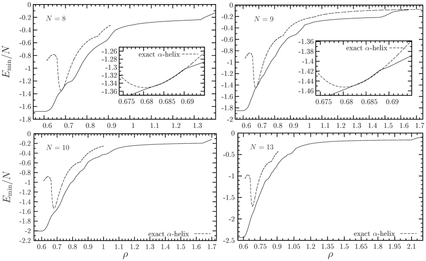
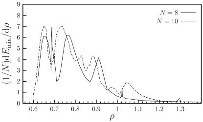
Figure 1 shows the energies of the ground states for various chain lengths in dependence of $\rho$ in comparison to the energy of the corresponding calculated space-filling (perfect) $\alpha$-helix. This helix is defined as the helix $(x,y,z)=(r\sin\phi,r\cos\phi,p\phi/2\pi)$ with a pitch $p$ such that the surface of the tube has a self-contact at the cylinder with radius $r$ and the radius $r$ is minimal under the thickness constraint. In other words, the optimally packed, i.e., space-filling, $\alpha$-helix corresponds to the transition between the two qualitatively different regimes of $p/r>c^{*}$ and $p/r\ll 1$ [37]. The computation of this helix is non-trivial, as the critical ratio $c^{*}$ depends on the discretization level and ranges from $c^{*}\approx 2$ for $\rho\approx 0.7$ to $c^{*}=2.512$ for the continuous case, which is equivalent to $\rho\to\infty$. An interesting and detailed discussion of compact helix formation and the critical ratio $c^{*}$ can be found also in [21].

Figure 3: Ground-state conformations for selected thickness parameters $\rho$ for $N=8$, $9$, $10$ and $13$ (from top to bottom). The second row for $N=8$ shows the same ground states with appropriate thickness, to give a better idea of the “real” objects we are investigating. The second rows for $N=9$ and $N=13$ show an alternative view of the same configuration. For reasons of better visibility, the thickness is not shown in the proper scale (except for the second row).

Figure 4: Contact maps of the conformations shown in Fig. 3. The axes show the monomer numbers $i$ and $j$, the entries of the matrix are set ($\bullet$), if two monomers $i$ and $j$ are in contact with each other, i.e., if the distance between them in the three-dimensional structure is shorter than a certain threshold value. This value is here slightly larger than the minimum distance of the LJ potential $r_{ij}^{\mathrm{min}}$.

Figure 5: End-to-end distances of ground-state conformations depending on the thickness constraint $\rho$. The dashed line for $N=9$ shows for comparison the end-to-end distance for the exact $\alpha$-helix.

Figure 6: Mean torsional angles of ground-state conformations depending on the thickness constraint $\rho$. Shown are absolute mean values of $\phi$ and $\phi_{\pi/2}:=\min(|\phi|,\pi-|\phi|)$. The short-dashed line for $N=9$ shows the behavior for the exact $\alpha$-helix.

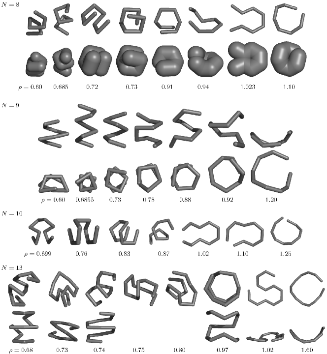
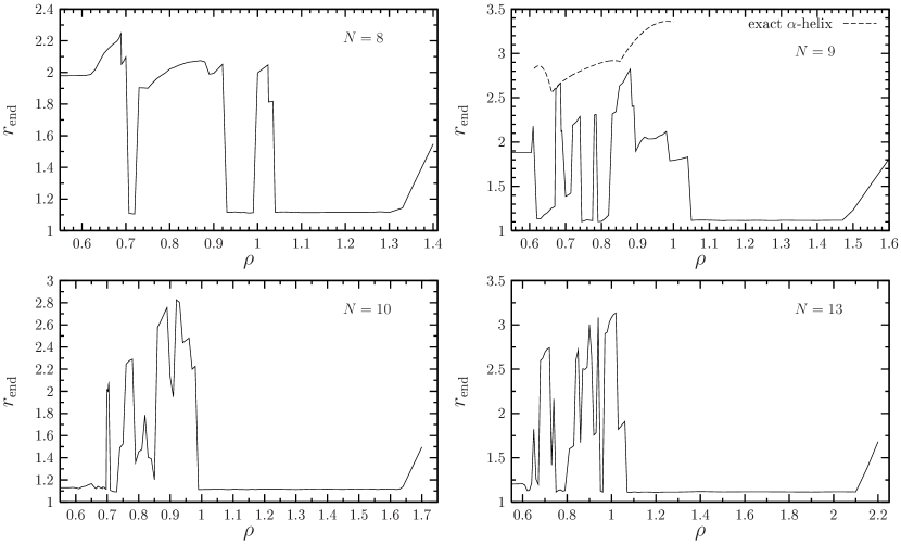
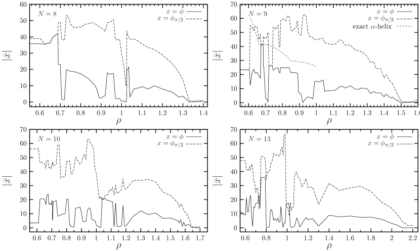
For two exemplified chain lengths, $N=8$ and $N=10$, we have plotted in Fig. 2 the derivatives $\mathrm{d}E/\mathrm{d}\rho$ in order to emphasize regions of structural activity. In these regions, where the derivative exhibits peaks, noticeable qualitative conformational transitions occur. To describe and understand these different classes of ground-state conformations, we visualize in Fig. 3 significant structures and plot in Fig. 4 the contact maps, where a contact is counted, if the distance between two monomers $r_{ij}<r_{ij}^{\mathrm{min}}+\epsilon$. We set $\epsilon\approx 0.2$ but, of course, the contact maps do not depend on minor variations of $\epsilon$. In addition, in Figs. 5 and 6 end-to-end distances and mean torsional angles discussed above are shown. Based on this data, we can classify the generic behavior by introducing three general regions: thin, intermediate, and thick tubes. Let us now look at these regions in more detail.

3.2.1 Thin tubes

The thin-tubes region is, besides some singular points, dominated by helical and helicallike conformations. We call a conformation “helical”, if $\bar{\phi}=\bar{\phi}_{\pi/2}$, where $\bar{x}$ is the average along the chain, $\bar{x}=(1/N)\sum_{i}x_{i}$, i.e., if all torsion angles lie in a range $0\dots\,\pm\pi/2$ (cp. Eq. (6) and Fig. 6; we do not distinguish between right- and left-handed helices, but the sign must not change within the conformation). Furthermore, the entries in the contact map lie precisely parallel to the diagonal of the matrix in these cases, a clear indication for helix structures (see, for example, $N=8;\rho=0.685$ or $N=9;\rho=0.73$ in Fig. 4). “Helicallike” conformations share some properties with helical structures, e.g., they exhibit a large, slightly increasing end-to-end distance (cp. Fig. 5) with increasing thickness, but the torsion-angle criterion above may be violated (typically in a periodical manner) and the contact-map entries do not form an exact parallel, but a line roughly parallel to the diagonal (for example, at $N=8;\rho=0.6$ or $N=9;\rho=0.78$). Generally, we find three interesting effects looking at the contact maps in Fig. 4, which have been mentioned above or will be discussed later again: First we see, that polymer chains without thickness constraint (see the maps for $N=8$ and $N=9$ with $\rho=0.6$) do not have a pronounced structure. Just by increasing the thickness a bit, clear helical structures emerge, indicated by straight “lines” parallel to the diagonal of the map (cp. $N=8$ and $N=9$ with $\rho=0.685(5)$). Secondly, by increasing the thickness further, we see, for example for $N=9$, that this parallel “lines” moves away from the diagonal, i.e., the helical conformations are “untwisting”. Finally, looking at the contact maps for $N=13$, we see that tertiary effects come into play, indicated by “disrupting” vertical “lines”, which is typically an indication for sheetlike structures.

Remarkably, within certain intervals ($N=8$: $0.63\leq\rho\leq 0.688$; $N=9$: $0.673\leq\rho\leq 0.6855$), the ground-state conformations expand with increasing thickness to a perfect space-filling helix with $\kappa_{0}$- and $\tau_{0}$-property, i.e., an $\alpha$-helix with constant bond- and torsion angles ($\bar{\phi^{2}}-\bar{\phi}\,\bar{\phi}$ and $\bar{r^{2}}_{\mathrm{lc}}-\bar{r}_{\mathrm{lc}}\bar{r}_{\mathrm{lc}}$ vanish). The comparison of measured observables with the data for the exact $\alpha$-helix is emphasized in the insets of Fig. 1 and furthermore exemplarily shown in Figs. 5 and 6. We will resume the discussion on this fact in Sect. 3.3.2 below.

As a remark: What is the motivation to call these conformations $\alpha$-helical in imitation of the real biological $\alpha$-helix? In natural proteins, $\alpha$-helices possess about $3.6$ amino acids per helix turn [38] and have mainly constant bond and torsion angles. If we construct a perfect space filling helix with exactly 3.6 monomers per turn, we find that it has a global radius of curvature of $r_{\mathrm{gc}}\approx 0.69$. Or, the other way around in the region $0.6845\leq\rho\leq 0.688$ (example for $N=8$), one counts $3.576\ldots 3.596$ monomers per turn, which is in very good agreement with natural $\alpha$-helices. We thus see the first biological relevant structure realized by the simplest model with just Lennard–Jones interaction and thickness but without any conformational assumptions or additional input.

An above mentioned singular point is located in the vicinity of the perfect helices at $\rho\approx 1/\sqrt{2}\approx 0.71$, where ground states attempt to crystallize in a regular simple cubic (sc) lattice structure. We find for example for $N=8$ at $\rho=0.73$ a $\kappa_{0}$-conformation almost fitting the sc lattice (elsewhere called “simple cubic lattice helix” [39]), which then untwists with increasing thickness. We see the same tendency for longer chains as well (see Fig. 3 for visualizations and Sect. 3.3.2 for further discussion). Note that a perfect cube will not be a ground state at any thickness, as the Lennard–Jones interaction length scale is larger than the bond length. If we reconfigure the potential such that its minimum value equals the bond length, i.e. set $r_{ij}^{\rm min}=1$, we find indeed that the ground-state conformations fit exactly into the simple cubic lattice (i.e. are exact cubes for adequate monomer numbers) up to lengths of $\approx 30$ monomers. We will show this in more detail in Sect. 3.3.1.

At larger thickness we observe in Fig. 3 extended helicallike conformations, which may overlap due to the shortness of the chains only at the end bonds.

3.2.2 Intermediate tubes

In the interval $0.9\lesssim\rho\lesssim 1.0$, we observe an abrupt switch to almost flat (cp. Fig. 6) and mostly closed (cp. Fig. 5) conformations. One finds bended double-rings, hairpins, and even conformations that are “crystallized” on a two-dimensional honeycomb lattice (cp. Fig. 3, $N=8$, $13$, $\rho\approx 1.02$). These curves are, of course, $\kappa_{0}$-curves as well and have apparent similarities to $\beta$-sheets known from secondary structures of biopolymers. We find in some small regions competitions between mesomeric structures, i.e. structures with the same monomer positions but different bond distributions (see, for example, Fig. 3, $N=10$, $\rho\approx 1.1$).

3.2.3 Thick tubes

At $\rho\approx 1.1$, the ground-state conformation is (again) “closed” for all chain lengths. Here begins the region of the twisted circles of constant curvature (“windschiefe Kreise”) [36, 35]. With increasing thickness, the rings become more and more flat until they reach the two-dimensional ring at $\rho\approx N/2\pi$, which is again a $\kappa_{0}$- and $\tau_{0}$-curve. Increasing thickness just pushes apart the ring, what can clearly be seen in the end-to-end distance and the torsion angles (see Figs. 5 and 6). For the somehow pathological case of $\rho\to\infty$ one would reach the limit of stiff rods.

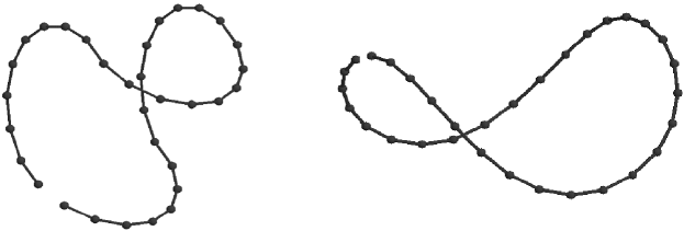
For purposes of illustration we display two examples from the class “windschiefe Kreise”. The first kind consists out of 4 half circles, which form a closed three-dimensional curve. The left side of Fig. 7 displays a $N=32$ chain, which is a ground state of the theory and has been obtained from simulations at $r_{\rm gc}=2.562915$ and $r_{ij}^{\rm min}=1.6$. As can be seen each of the half-circles consists of eight monomers. The second kind of “windschiefe Kreise” consists out of four helix sections, that are joined together in such a way that the resulting curve is closed again. The right side of Fig. 7 displays such a $N=32$ chain, which was obtained from simulations at $r_{\rm gc}=3.624510$ and $r_{ij}^{\rm min}=1.6$.

Figure 7: Two examples for twisted circles of constant curvature $r_{\rm c}\approx 2.6$ (left) and $r_{\rm c}\approx 3.6$ (right) with $N=32$ monomers. See text for details.

3.2.4 General remarks

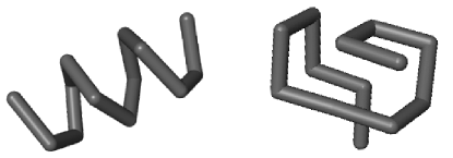
It is not surprising, that the situation becomes more complex with increasing chain length. At least some of the described “nice-looking phases” above are artificial in the sense, that they occur at exactly one short length, or are favored just by that very short length, respectively. We see, for example, for $N=10$ and $N=13$ no exact ($\alpha$-)helices anymore, it rather seems that at these lengths “tertiary” effects already play a role in the sense, that two small secondary structures are formed which are then arranged “side by side”. An indication for this trend may be that conformations with low thickness are often “symmetric”, i.e., the conformations get buckled and turn back at some point (generally in the middle). See for example the helical region for $N=13$ in Fig. 3. Anyhow, the helical structures being present for shorter chains indeed exist “very close” to the ground states, i.e., with a slightly higher energy. Two of these conformations are depicted in Fig. 8.

We will get further convincing arguments for this classification scheme by investigating the thermodynamic behavior of these polymers in the aforementioned general structural phases [32, 31]. The transition lines between the phases then depend indeed on both thickness and temperature. For low temperatures, the helical phase corresponds to polymers with low thickness, the sheet phase to a little higher thickness and the ring phase to the very thick polymers.

Figure 8: Two $N=13$ conformations with $\rho=0.73$ (left) and $\rho=0.74$ (right), which are not the ground-state conformations but have a just slightly higher energy than these. The conformations correspond to distinguished ground-state structures at shorter lengths (helical and crystallized on the sc lattice, cp. Fig. 3). For reasons of better visibility, the thickness is not shown on scale.

3.3 Selected Problems: Deeper Analysis and Remarks

3.3.1 Simple cubic symmetry

One of the basic observations within our polymer model relates to the fact, that the theory’s parameter space of thickness $\rho$ and $r_{ij}^{\rm min}$ values possibly contains a likewise finite set of isolated and special parametric points, for which ground-state conformations exhibit a strict crystalline structure. These polymer conformations are characterized by a point set of monomer positions, that is frozen into a regular three-dimensional (3d) structure and none positional degree of freedom is left over. Additionally, these ground states inherit a finite and possibly large ground-state degeneracy as there exist many ways to arrange the polymers sequence of monomers onto the frozen point set, without lifting the theory’s energy to larger values. Typically, we then expect a number of ground-state configurations that increases exponentially, $n_{0}\propto{\rm exp}(cN)$, with the chain length for long chains. Furthermore, the presence of crystalline ground states in the tube model possibly is attached to a triplet of global radius values $r_{\rm gc}=0.5774$, $1/\sqrt{2}=0.7071$, and $r_{\rm gc}=1$, which denote the radii of circular polymers, that have an end-to-end distance of unity with exactly $N=3$, $4$, and $N=6$ monomers on a circle. With numerical means it is then easy to show, that these particular radii result into triangular lattice ($N=3$), simple square lattice ($N=4$), and honeycomb lattice ($N=6$) ground-state polymer point sets in two dimensions (2d), that is to say dimensional reduced tube polymer model. The phase space of 3d polymers as such is much larger than in 2d and a search at $r_{\rm gc}=0.5774$ and $r_{\rm gc}=1$ does not reveal any crystals for 3d polymers that would persist in the thermodynamic limit. However, at the particular value of $r_{\rm gc}=1/\sqrt{2}$ and for $r_{ij}=1$, we find stable 3d ground-state conformations with point sets of simple cubic symmetry and with large ground-state degeneracy. These crystals are likely to extend in the thermodynamic limit for large $N$ values.

The numerical simulations in case of the 3d thick tube model have been performed on chain length values $N=8,9,\ldots,32,36,40,44,48,52,56,60$, and $N=64$. The global radius parameter was chosen to be $\rho=1/\sqrt{2}$ with the value $r_{ij}^{\rm min}=1$ for the position of the Lennard–Jones potential minimum. We employed parallel tempering simulations in the temperature interval $0.01\leq T\leq 0.5$ with a temperature partition, that ensures acceptance rates around $0.5$ for parallel tempering swaps in-between neighbors in the temperature. For complete temperature interval coverage on a $N=32$ chain a total of $39$ temperature replica was needed. A single Monte Carlo run consists out of $10^{9}\times N$ monomer positional updates and from the ensemble of configurations the minimum-energy configuration was stored. A sequence of about $10$ continuation runs for each chain length $N$ with identical run parameters but with continued start configurations then yields an ensemble of about $10$ ground-state estimates, and also the global ground-state estimate of the simulation. Finally, an adapted conjugate-gradient method was applied for refinement. We found that the efficiency of the Monte Carlo simulation in an attempt to populate statistically independent ground states rapidly degrades for chain length values $N\geq 36$ and therefore the longest chains (except the one at $N=36$) are excluded from the further analysis.

Figure 9: A ground-state conformation for the $N=27$ polymer with $\rho=1/\sqrt{2}$ and $r_{ij}^{\rm min}=1$ (i.e., $\sigma\neq 1$). The left picture shows the conformation in the proper scale, the right side shows the same conformation without proper thickness.

For a crystalline polymer conformation with simple cubic symmetry one can find a set of transformations, i.e., translations and orthochroneous rotations, that map the polymers point set to some point set of a simple hypercubic lattice. Denoting by $\vec{x}_{i}^{\,\rm sc}=m_{i}^{\alpha}\vec{e}_{\alpha}$ with $i=1,\ldots,N$, $\alpha=1,2,3$, and with $m_{i}^{\alpha}$ integer, a point set on a simple cubic lattice, the mean squared distance to a simple cubic lattice

$$d_{\rm sc}^{2}={1\over N}\sum_{i=1}^{N}(\vec{x}_{i}^{\rm polymer}-\vec{x}_{i}^{\,\rm sc})^{2}$$ (7)

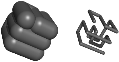
can be transformed to $d_{\rm sc}^{2}=0$, if also an appropriate set of $m_{i}^{\alpha}$ values is chosen. Our main numerical result consists in the finding that all of our ground-state polymers at $N=8,9$ and for $N=11,12,\ldots,36$ fulfill the numerically determined inequality $d_{\rm sc}^{2}\leq 0.000053$ and therefore we observe a blatant simple hypercubic symmetry in the ground state of the theory for the considered chain length values to a high degree of numerical precision. A particular impressive ground-state conformation is displayed in Fig. 9, where the $N=27$ polymer folds onto a $3\times 3\times 3$ cuboid: ${\rm Cub}(3\times 3\times 3)$. For the $N=27$ chain, we performed a total of eight different continuation runs, which all yielded simple cubic symmetry in the ground-state estimates with values $d_{\rm sc}^{2}\leq 0.000053$. From these eight configurations, six were found with point sets isomorphic to ${\rm Cub}(3\times 3\times 3)$, however with five different mappings of the polymer sequence to the cuboid and with almost degenerate energy close to the ground-state energy. Given the numerical ability of the algorithm to identify different ground-state and near-by ground-state conformations, it appears unlikely that the true ground state has not been identified for the $N=27$ chain. A similar remark applies to all shorter chains. For purposes of future reference, and as a yard stick of our numerical precision we display in Table 1 ground-state energy density values $e_{0}=E/N$ from numerical simulations (second row) as a function of the chain length $N$, as well as exactly calculated energy densities for various cuboids. It is noteworthy that ground states at $N=8,12$ and $N=18$ also exhibit cuboidal point sets: ${\rm Cub}(2\times 2\times 2),{\rm Cub}(2\times 2\times 3)$ and ${\rm Cub}(2\times 3\times 3)$ respectively. For the $N=36$ chain the exactly calculated energy density of the ${\rm Cub}(3\times 3\times 4)$ cuboid undershoots the numerical value significantly and, in fact, the cuboid was not found in the numerical simulations. This again indicates the failure of our numerical algorithms for chains with length $N\geq 36$. Finally, it is also of interest to classify the secondary structures of compactified ground-state conformations for the case of simple cubic symmetries. In particular we may consider U-turns (planar), and simple cubic helices (3-dimensional) [39], which both are chain segments of four monomers with bending angles of $90$-degrees in-between consecutive segments on the simple cubic lattice. Using a pattern recognition program along the ideas of Tenenbaum et al. [40] on a set of five different ground-state conformations for the $N=27$ polymer we obtain rather low probabilities $P_{\rm U-turn}\approx 0.27$ and $P_{\rm sc-helix}\approx 0.22$ for the occurrence of U-turns and sc-helices, respectively.

Table 1: Ground-state energy density values $e_{0}=E/N$ from numerical simulations (second row) as a function of the chain length $N$, as well as exactly calculated energy densities $e_{0}({\rm cuboids})$ for various cuboids (fourth row).

$N$	$e_{0}$	${\rm Manifold}$	$e_{0}({\rm cuboids})$
8	$-1.0032$	${\rm Cub}(2\times 2\times 2)$	$-1.0038$
9	$-0.9670$
10	$-1.0398$
11	$-1.1052$
12	$-1.2497$	${\rm Cub}(2\times 2\times 3)$	$-1.2514$
13	$-1.2263$
14	$-1.2773$
15	$-1.3179$
16	$-1.4152$
17	$-1.4451$
18	$-1.5267$	${\rm Cub}(2\times 3\times 3)$	$-1.5293$
19	$-1.5165$
20	$-1.5496$
21	$-1.5729$
22	$-1.6346$
23	$-1.6612$
24	$-1.7159$
25	$-1.7465$
26	$-1.7944$
27	$-1.8385$	${\rm Cub}(3\times 3\times 3)$	$-1.8433$
28	$-1.8230$
29	$-1.8282$
30	$-1.8383$
31	$-1.8750$
32	$-1.8875$
36	$-1.9224$	${\rm Cub}(3\times 3\times 4)$	$-2.0036$

3.3.2 The $\alpha$-helix region

For the $N=8$ and $9$ polymer, we found a thickness region, where the $\alpha$-helix is the ground-state conformation (see Sect. 3.2). Remember that we used the Lennard–Jones potential with $\sigma=1$ there, which sets the interaction length scale. There is nothing special with it, except that the potential just vanishes at the bond length, a fact that plays just a “second order” role, as we are not counting energy contribution from consecutive monomers at all.

Figure 10: $N=8$: The $\sigma$–$\rho$ plane and ground-state conformations near the $\alpha$-helix. The left and right coordinates are connected just via $r_{ij}^{\rm min}=2^{1/6}\sigma$. See text for details.

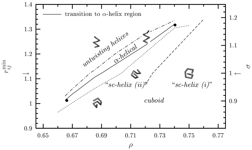
Because of the special role of the $\alpha$-helix in nature (besides its geometrical elegance), we will here try to track the $\alpha$-helix not only in the thickness but also in the $\sigma$-direction of the “phase space”, i.e. we vary $\rho$ and $\sigma$ independently in the vicinity of the assumed “$\alpha$-region”. Our results are displayed, exemplarily for $N=8$, in Fig. 10. We see, that the $\alpha$-helix occurs as ground-state conformation in a small, bounded thickness interval ($0.66<\rho<0.75$) right “before” an abrupt conformational change (depicted by the solid line) to cubelike structures. The transition line increases approximately linearly in the interaction-length–thickness plane, a dependence, which seems to hold generally for structural transitions in the vicinity. Following a perpendicular path, i.e., with increasing interaction lengths and decreasing thickness, the helices untwist smoothly. The dashed-dotted line together with the solid line define the region, where the $\alpha$-helix is the ground state of the system (cp. insets in Fig. 1). Note that for $\rho<0.66$ and $\rho>0.75$, $\alpha$-helices are no ground states at all.

A further interesting transition is marked by the dashed line in Fig. 10. This line indicates the transition between the so-called simple cubic “lattice helices (ii)” and “(i)” [39], i.e., cuboidlike structures with parallel and antiparallel tails (remember that for $r_{ij}^{\rm min}=1$ and $\rho=1/\sqrt{2}$, we observe the “crystallization” exactly at the simple cubic lattice, as mentioned in Sect. 3.2.1 and in detail discussed in Sect. 3.3.1).

For the sake of completeness, the dotted line indicates a conformational change to some less interesting intermediate structure “between” $\alpha$- and lattice helices and the arrows on the $y$-axes mark the line $\sigma=1$ investigated in the first part of this study.

4 Summary

The aim of this work was to take the simplest coarse-grained model for off-lattice polymers with explicit volume exclusion and to show, to which degree polymer crystallization can be understood even with this simplest model. We introduced the polymer volume using the concept of the radius of curvature which is indeed, in the first instance, a mathematical concept. In fact, it has been proven that “[it] is connected to various physically appealing properties of a curve. In particular, [it] provides a concise characterization of the thickness of a curve, […] as have been investigated within the context of DNA” [19], it was further successfully used in more complex models for proteins [16, 17, 34] and it was finally shown, that this concept is effectively equal to a volume exclusion using two-point functions for polymers in good solvents [18].

Using sophisticated simulation techniques, we have analyzed systematically and in detail ground-state structures for the described model with fixed interaction length. We have shown, for example, that already in this simplest model basic secondary structures like helices and sheets form. This statement is, due to the simplicity of the model, valid for various classes of polymers. Of course, it should be stated as well, that mentioned structures are not very stable against variations of the thickness, but this was not expected either.

We investigated furthermore in detail the “neighborhood” of the $\alpha$-helix by varying both, thickness and interaction length. Affirming above statement, it turned out that the $\alpha$-helix exists as ground state only in a small, bounded area in the $\sigma$–$\rho$ space, but is surrounded by other helical and helicallike conformations.

It was of course known for a long time, that helices and sheets form within coarse-grained models including a somehow defined volume exclusion, but to our knowledge mainly for dedicated or less simple and not that general models. In some interesting works, for example, the strength of directionalized interactions [12], explicit hydrogen bonds [41, 42], solvent particles [20, 21, 22], or the interplay between attractive interactions and packing [14] play a role. In particular the findings of [14] also confirm the existence of not too long helical structures in a specific homopolymer model that is characterized by strong repulsive interactions between spheres. It is a common ansatz to investigate and understand protein folding, stressing that we do not speak only of proteins but of a general class of polymers including proteins, at different abstraction (coarse grained) levels. It seems that at least parts of the general secondary structure formation can be attributed already to the simplest generic model for thick polymers. Obviously, these secondary structure segments have to be strengthened by further interactions in order to reach, for example, biologically relevant structure sizes, as tertiary effects set in at comparatively short chain lengths in simple coarse-grained models [12, 21, 32].

The analysis of ground states is, of course, just a first step to an understanding of the model. In a subsequent work [32] we will, based on the knowledge of the ground-state conformations, focus on the thermodynamic behavior and conformational phases at finite temperatures.

Acknowledgement

This work is partially supported by the DFG (German Science Foundation) under Grant No. JA 483/24-1/2/3 and the Graduate School of Excellence “BuildMoNa”. Some simulations were performed on the supercomputer JUMP of the John von Neumann Institute for Computing (NIC), Forschungszentrum Jülich, under Grant No. hlz11.

References

- [1] M.N. Rosenbluth, A.W. Rosenbluth, J. Chem. Phys. 23, 356 (1955)
- [2] D.P. Landau, K. Binder, A Guide to Monte Carlo Simulations in Statistical Physics, 2nd edn. (Cambridge University Press, New York, 2005)
- [3] D. Frenkel, B. Smit, Understanding Molecular Simulation, 2nd edn. (Academic Press, 2002)
- [4] S. Gnanakaran, H. Nymeyer, J. Portman, K.Y. Sanbonmatsu, A.E. García, Curr. Opin. Struct. Biol. 13, 168 (2003)
- [5] W. Janke, ed., Rugged Free Energy Landscapes (Springer, Berlin, 2008), Vol. 736 of Lecture Notes in Physics, chap. 10, 11 and 14
- [6] H.P. Hsu, P. Grassberger, Europhys. Lett. 77, 18003 (2007)
- [7] W. Paul, T. Strauch, F. Rampf, K. Binder, Phys. Rev. E 75, 060801(R) (2007)
- [8] S. Schnabel, M. Bachmann, W. Janke, Phys. Rev. Lett. 98, 048103 (2007)
- [9] S. Schnabel, T. Vogel, M. Bachmann, W. Janke, Chem. Phys. Lett. 476, 201 (2009)
- [10] P. Grassberger, Phys. Rev. E 56, 3682 (1997)
- [11] T. Vogel, M. Bachmann, W. Janke, Phys. Rev. E 76, 061803 (2007)
- [12] J.P. Kemp, Z.Y. Chen, Phys. Rev. Lett. 81, 3880 (1998)
- [13] H. Noguchi, K. Yoshikawa, J. Chem. Phys. 109, 5070 (1998)
- [14] J.E. Magee, V.R. Vasquez, L. Lue, Phys. Rev. Lett. 96, 207802 (2006)
- [15] S.A. Sabeur, F. Hamdache, F. Schmid, Phys. Rev. E 77, 020802(R) (2008)
- [16] J.R. Banavar, A. Flammini, D. Marenduzzo, A. Maritan, A. Trovato, J. Phys. Cond. Mat. 15, S1787 (2003)
- [17] J.R. Banavar, A. Maritan, Rev. Mod. Phys. 75, 23 (2003)
- [18] T. Neuhaus, O. Zimmermann, U.H.E. Hansmann, Phys. Rev. E 75, 051803 (2007)
- [19] O. Gonzalez, J.H. Maddocks, Proc. Natl. Acad. Sci. USA 96, 4769 (1999)
- [20] Y. Snir, R.D. Kamien, Science 307, 1067 (2005)
- [21] Y. Snir, R.D. Kamien, Phys. Rev. E 75, 051114 (2007)
- [22] H. Hansen-Goos, R. Roth, K. Mecke, S. Dietrich, Phys. Rev. Lett. 99(12), 128101 (2007)
- [23] B.A. Berg, T. Neuhaus, Phys. Lett. B 267, 249 (1991)
- [24] B.A. Berg, T. Neuhaus, Phys. Rev. Lett. 68, 9 (1992)
- [25] E. Bittner, W. Janke (2009), in preparation
- [26] F. Wang, D.P. Landau, Phys. Rev. Lett. 86, 2050 (2001)
- [27] C. Zhou, R.N. Bhatt, Phys. Rev. E 72, 025701(R) (2005)
- [28] K. Hukushima, K. Nemoto, J. Phys. Soc. Jpn. 65, 1604 (1996)
- [29] C.J. Geyer, in Computing Science and Statistics, Proceedings of the 23rd Symposium on the Interface, edited by E.M. Keramidas (Interface Foundation, Fairfax Station, 1991), p. 156
- [30] W.H. Press, S.A. Teukolsky, W.T. Vetterling, B.P. Flannery, Numerical Recipes: The Art of Scientific Computing (Cambridge University Press, Cambridge, 2007), chap. Conjugate Gradient Methods in Multidimensions, p. 515, 3rd edn.
- [31] T. Vogel, T. Neuhaus, M. Bachmann, W. Janke, EPL (Europhys. Lett.) 85, 10003 (2009)
- [32] T. Vogel, T. Neuhaus, M. Bachmann, W. Janke, Phys. Rev. E 80, 011802 (2009)
- [33] J.R. Banavar, A. Maritan, C. Micheletti, A. Trovato, Proteins 47, 315 (2002)
- [34] J.R. Banavar, O. Gonzalez, J.H. Maddocks, A. Maritan, J. Stat. Phys. 110, 35 (2003)
- [35] R. Koch, C. Engelhardt, J. Geom. Graph. 2(1), 17 (1998)
- [36] E. Cesàro, Vorlesungen über natürliche Geometrie (Teubner, Leipzig, 1926), 2nd edn.
- [37] A. Maritan, C. Micheletti, A. Trovato, J.R. Banavar, Nature 406, 287 (2000)
- [38] A.L. Lehninger, D.L. Nelson, M.M. Cox, Principles of Biochemistry, 2nd edn. (Worth Publishers, New York, 1992)
- [39] H.S. Chan, K.A. Dill, J. Chem. Phys. 92(5), 3118 (1990)
- [40] J.B. Tenenbaum, V. de Silva, J.C. Langford, Science 290, 2319 (2000)
- [41] T.X. Hoang, A. Trovato, F. Seno, J.R. Banavar, A. Maritan, Proc. Natl. Acad. Sci. USA 101(21), 7960 (2004)
- [42] K. Wolff, M. Vendruscolo, M. Porto, Gene 422(1–2), 47 (2008)