On the dynamics of multiple systems of hot super–Earths and Neptunes: Tidal circularization, resonance and the HD 40307 system

Abstract

In this paper, we consider the dynamics of a system of hot super–Earths or Neptunes such as HD 40307. We show that, as tidal interaction with the central star leads to small eccentricities, the planets in this system could be undergoing resonant coupling even though the period ratios depart significantly from very precise commensurability. In a three planet system, this is indicated by the fact that resonant angles librate or are associated with long term changes to the orbital elements. In HD 40307, we expect that three resonant angles could be involved in this way. We propose that the planets in this system were in a strict Laplace resonance while they migrated through the disc. After entering the disc inner cavity, tidal interaction would cause the period ratios to increase from two but with the inner pair deviating less than the outer pair, counter to what occurs in HD 40307.

However, the relationship between these pairs that occurs in HD 40307 might be produced if the resonance is impulsively modified by an event like a close encounter shortly after the planetary system decouples from the disc. We find this to be in principle possible for a small relative perturbation on the order of a few $\times 10^{-3}$ but then we find that evolution to the present system in a reasonable time is possible only if the masses are significantly larger than the minimum masses and tidal dissipation is very effective. On the other hand we found that a system like HD 40307 with minimum masses and more realistic tidal dissipation could be produced if the eccentricity of the outermost planet was impulsively increased to $\sim 0.15.$

We remark that the form of resonantly coupled tidal evolution we consider here is quite general and could be of greater significance for systems with inner planets on significantly shorter orbital periods characteristic of for example CoRoT 7 b.

1 Introduction

Neptune mass extrasolar planets around main sequence stars were first detected five years ago. Since then, 27 planets with a projected mass lower than 25 earth masses have been discovered, the lightest one having a projected mass of 1.94 M_⊕. Among these objects, 17 have a semi–major axis smaller than 0.1 astronomical unit (au). They are called hot Neptunes or hot super–Earths. So far, two multiple planet systems with at least two such objects have been observed. One of them is a four planet system around the M–dwarf GJ 581 (Bonfils et al. 2005, Udry et al. 2007, Mayor et al. 2009a). The projected masses of the planets are 1.9, 15.6, 5.4 and 7.1 M_⊕ and the periods are 3.15, 5.37, 12.93 and 66.8 days, respectively. Note that although the eccentricities of the two innermost planets are compatible with zero, those of the next outermost and outermost planets are 0.16 and 0.18 respectively. The second multiple system which we shall focus upon in this paper is that around the K–dwarf HD 40307 (Mayor et al. 2009b). It comprises three planets with projected masses of 4.2, 6.9 and 9.1 M_⊕ and periods of 4.31, 9.62 and 20.46 days, respectively. The eccentricities are all compatible with zero.

If we label the planets in a system with successive integers starting from the innermost labelled, 1, and moving outwards, then, in the system Gl 581, the ratio of the periods of planets 2 and 1 is 2.41 and that of the periods of planets 3 and 2 is 1.70. We note that these numbers depart from 5/2 and 5/3 only by 4% and 2%, respectively.a In the HD 40307 system , the ratio of the periods of planets 2 and 1 is 2.23 and that of planets 3 and 2 is 2.13, which depart from 2 by 11.5% and 6.5%, respectively. Because departure from exact mean motion resonances in these systems is significant, the importance of resonances for their dynamical evolution has been ruled out (Mayor et al. 2009a, 2009b, Barnes et al. 2009). We shall address this aspect for the HD 40307 system in this paper.

Migration due to tidal interaction with the disc is probably the mechanism by which planets end up on short period orbits, as in situ formation requires very massive discs (e.g., Raymond et al. 2008). Planet–planet scatterings may also lead to short period orbits, but only when tidal circularization is efficient. According to Kennedy & Kenyon (2008), scatterings are not a likely way of producing hot super–Earths, because of the long circularization timescales involved. In a previous paper (Terquem & Papaloizou 2007, see also Brunini & Cionco 2005), we proposed a scenario for forming hot super–Earths on near commensurable orbits, in which a population of cores that assembled at some distance from the central star migrated inwards due to tidal interaction with the disc while merging on their way in. We found that evolution of an ensemble of cores in a disc almost always led to a system of a few planets, with masses that depended on the total initial mass of the system, on short period orbits with mean motions that frequently exhibited near commensurabilities and, for long enough tidal circularization times, apsidal lines that were locked together. Starting with a population of 10 to 25 planets of 0.1 or 1 M_⊕, we ended up with typically between two and five planets with masses of a few tenths of an earth mass or a few earth masses inside the disc inner edge. Interaction with the central star led to the initiation of tidal circularization of the orbits which, together with possible close scatterings and final mergers, tended to disrupt mean–motion resonances that were established during the migration phase. The system, however, often remained in a configuration in which the orbital periods were close to commensurability. Apsidal locking of the orbits, if established during migration, was often maintained through the action of these processes.

This scenario has been questioned (Mayor et al. 2009a, 2009b) because the multiple planet systems of hot super–Earths detected so far do not exhibit close enough mean motion commensurabilities. In this paper, we argue that the system around HD 40307 does actually exhibit the effects of resonances through secular effects produced by the action of the resonant angles coupled with the action of tides from the central star, and that such a configuration could be produced if the system formed as described in Terquem & Papaloizou (2007), but with the addition of relatively small perturbations to the orbits arising from close encounters or collisions after the system enters the disc inner cavity. The reason that what are regarded as resonant effects can arise even when departures from strict commensurability are apparently large is that tidal circularization produces small eccentricities which, for first order resonances, can be consistent with resonant angle libration under those conditions (see Murray & Dermott 1999).

We consider in detail the evolution of this system and other putative similar systems with scaled masses and orbital periods after they form a strict three planet Laplace resonance as a result of convergent inward orbital migration. We go on to consider the onset of tidal circularization and how it leads to a separation of the semi-major axes and consequent increasing departure from commensurability. We find that if the strict Laplace resonance is broken by a fairly small relative perturbation corresponding to a few parts in a thousand, continuing evolution in a modified form of the three planet resonance could in principle in the case of HD 40307 lead to a system like the observed one. However, this would require masses significantly larger than the minimum estimates and possibly unrealistically efficient tidal dissipation with the tidal dissipation parameter $Q^{\prime}\sim 10.$ However, weaker tidal effects could be responsible for some of the deviation from strict commensurability, with the rest being produced by a larger perturbation resulting from the processes mentioned above inducing eccentricities of the order $0.1.$ Note however that tidal evolution could play a more significant role in similar systems with shorter orbital periods.

In section 2, we describe the numerical model we use to simulate the evolution of a system of three planets migrating in a disc and evolving under the tidal interaction with the star after they enter the disc inner cavity. In section 3, we simulate the system around HD 40307 using either the minimum or twice the minimum masses for the planets under varying assumptions about initial eccentricities and the strength of the tidal interaction. We show that three of the four possible resonant angles associated with 2:1 commensurabilities either librate or have long term time averages, indicating evolution of the system towards a resonant state driven by the tidal influence of the star.

In a related appendix, we give a semi–analytic model for a system in a three planet resonance undergoing circularization with departures from strict mean motion commensurabilities. We note in passing that the discussion may also be applied to a two planet system near a 2:1 resonance. We show that the departure from commensurability increases with time being $\propto t^{1/3}$ and derive an expression for the timescale required to attain a given departure that can be used to interpret extrapolate from and generalize the numerical simulations.

In section 4, we present results of numerical simulations of a three planet system migrating in a disc, establishing a 4:2:1 Laplace like resonance, and evolving under tidal effects induced by the star after entering the disc inner cavity. As expected, as the orbits are being tidally circularized, the planets move away from exact commensurabilites, and the period ratios of the outer and inner pairs of planets increases.

The system is still resonant in the sense that some of the resonant angles continue to librate. To get a larger period ratio for the inner pair of planets, as in HD 40307, some disruption of this Laplace resonant state is needed. In our simulations, this is achieved by applying an impulse (that could result from an encounter or collision) to the system. This leads to departures from exact commensurabilites of the form seen in HD 40307 while still retaining libration of three of the four resonant angles. Finally, in section 5 we discuss and summarize our results.

2 Model and initial conditions

The model we use has been described in Terquem & Papaloizou (2007). We recall here the main features. We consider a system consisting of a primary star and N planets embedded in a gaseous disc surrounding it (for HD 40307, N =3). The planets undergo gravitational interaction with each other and the star and are acted on by tidal forces from the disc and the star. The evolution of the system is studied by means of the solution of $N$–body problems, in which the tidal interactions are included as dissipative forces.

The equations of motion are:

$${d^{2}{\bf r}_{i}\over dt^{2}}=-{GM_{\star}{\bf r}_{i}\over|{\bf r}_{i}|^{3}}-\sum_{j=1\neq i}^{N}{Gm_{j}\left({\bf r}_{i}-{\bf r}_{j}\right)\over|{\bf r}_{i}-{\bf r}_{j}|^{3}}-{\bf\Gamma}+{\bf\Gamma}_{i}+{\bf\Gamma}_{r}\;,$$ (1)

where $M_{\star}$, $m_{j}$ and ${\bf r}_{j}$ denote the mass of the central star, that of planet $j$ and the position vector of planet $j$, respectively. The acceleration of the coordinate system based on the central star (indirect term) is:

$${\bf\Gamma}=\sum_{j=1}^{N}{Gm_{j}{\bf r}_{j}\over|{\bf r}_{j}|^{3}},$$ (2)

and that due to tidal interaction with the disc and/or the star is dealt with through the addition of extra forces as in Papaloizou & Larwood (2000):

$${\bf\Gamma}_{i}=-\frac{1}{t_{m,i}}\frac{d{\bf r}_{i}}{dt}-\frac{2}{|{\bf r}_{i}|^{2}t_{e,i}}\left(\frac{d{\bf r}_{i}}{dt}\cdot{\bf r}_{i}\right){\bf r}_{i}-\frac{2}{t_{i,i}}\left(\frac{d{\bf r}_{i}}{dt}\cdot{\bf e}_{z}\right){\bf e}_{z},$$ (3)

where $t_{m,i}$, $t_{e,i}$ and $t_{i,i}$ are the timescales over which, respectively, the angular momentum, the eccentricity and the inclination with respect to the unit normal ${\bf e}_{z}$ to the assumed fixed gas disc midplane change. Evolution of the angular momentum and inclination is due to tidal interaction with the disc, whereas evolution of the eccentricity occurs due to both tidal interaction with the disc and the star. We have:

$$\frac{1}{t_{e,i}}=\frac{1}{t_{e,i}^{d}}+\frac{1}{t_{e,i}^{s}},$$ (4)

where $t_{e,i}^{d}$ and $t_{e,i}^{s}$ are the contribution from the disc and tides raised by the star, respectively. Relativistic effects are included through ${\bf\Gamma}_{r}$ ( see Papaloizou & Terquem 2001).

The way it is implemented, interaction with the star does not modify the angular momentum of a single orbit (the orbital decay timescale due to tidal interaction with the star, which as indicated below is estimated to be much longer than the circularization timescale, has been ignored here). However, in the formulation above, eccentricity damping causes radial velocity damping, which results in energy loss at constant angular momentum. As a consequence, both the semi–major axis and eccentricity are reduced together (at least for a single planet).

2.1 Orbital circularization due to tides from the central star

The circularization timescale due to tidal interaction with the star can be estimated, from expressions given by Goldreich & Soter (1966), to be:

$$t_{e,i}^{s}=4.065\times 10^{4}\;\left(\frac{{\rm M}_{\oplus}}{m_{i}}\right)^{2/3}\left(\frac{20a_{i}}{{\rm 1~{}au}}\right)^{6.5}Q^{\prime}\;\;\;{\rm years},$$ (5)

where $a_{i}$ is the semi–major axis of planet $i.$ Here we have adopted a mass density of 1 g cm³ for the planets (uncertainties in this quantity could be incorporated into a redefinition of $Q^{\prime}$). The parameter $Q^{\prime}=3Q/(2k_{2}),$ where $Q$ is the tidal dissipation function and $k_{2}$ is the Love number. Equation (5) applies to the situation where tides raised by the central star are dissipated in the planet in the limit of small eccentricity which is appropriate here. Tides raised by the planet in the star have been estimated to be unimportant for the low mass planets of interest (eg. Barnes et al 2009). For solar system planets in the terrestrial mass range, Goldreich & Soter (1966) give estimates for $Q$ in the range 10–500 and $k_{2}\sim 0.3$, which correspond to $Q^{\prime}$ in the range 50–2500. Of course this parameter must be regarded as being very uncertain for extrasolar planets, and accordingly we have considered values of $Q^{\prime}$ in the range $10-1000$ in this paper. For an earth mass planet at 0.05 au and $Q^{\prime}=50$, we get $t_{e,i}^{s}=2\times 10^{6}$ years. This indicates that circularization processes will be important for close in extrasolar planets in this mass range over the entire range of $Q^{\prime}$ considered.

But note that although circularization operates on each orbit according to equation (5), because the planets interact they may enter into a decay mode with a decay timescale that is not straightforwardly estimated as above (see section 3.1) . Nonetheless the above estimate is found to be indicative.

We have pointed out above that, in our formulation, tidal interaction with the star does not change the angular momentum of a single orbit but modifies the semi–major axis. The physical basis for this is that the planets rapidly attain pseudo-synchronization (e.g., Ivanov & Papaloizou 2007), after which they cannot store significant angular momentum changes through modifying their intrinsic angular momenta.

We restrict consideration for the moment to a single planet. Since the orbital angular momentum is conserved, $(da_{i}/dt)/a_{i}\simeq-2e_{i}^{2}/t_{e,i}^{s}$ for small eccentricities, where $e_{i}$ is the eccentricity of the planet we consider. Therefore $a_{i}$ changes only by about 5 percent in $10^{10}$ years for $Q^{\prime}=10,$ $m_{i}=1$ M_⊕ and $e_{i}=10^{-3}.$ However, larger changes may occur for larger planet masses. We investigate the dependence of this form of evolution on the system configuration in detail below.

Finally we remark that all the simulation results reported here were obtained assuming that $Q^{\prime}$ is the same for all the planets. However, tests were carried out with this assumption relaxed and these are alluded to in section 4 below.

2.2 Type I migration

In the local linear treatment of type I migration (e.g., Tanaka et al. 2002), if the planet is not in contact with the disc, there is no interaction between them so that $t_{m,i}$, $t_{e,i}^{d}$ and $t_{i,i}$ are taken to be infinite. When the planet is in contact with the disc, disc–planet interactions occur leading to orbital migration as well as eccentricity and inclination damping (e.g., Ward 1997). In that case, away from the disc edge, for some simulations we have adopted:

$$t_{m,i}=146.0\;\left[1+\left(\frac{e_{i}}{1.3H/r}\right)^{5}\right]\left[1-\left(\frac{e_{i}}{1.1H/r}\right)^{4}\right]^{-1}\;\left(\frac{H/r}{0.05}\right)^{2}\;\frac{{\rm M}_{\odot}}{M_{d}}\;\frac{{\rm M}_{\oplus}}{m_{i}}\;\frac{a_{i}}{{\rm 1~{}au}}\;\;\;{\rm years},$$ (6)

$$t_{e,i}^{d}=0.362\;\left[1+0.25\left(\frac{e_{i}}{H/r}\right)^{3}\right]\;\left(\frac{H/r}{0.05}\right)^{4}\;\frac{{\rm M}_{\odot}}{M_{d}}\;\frac{{\rm M}_{\oplus}}{m_{i}}\;\frac{a_{i}}{{\rm 1~{}au}}\;\;\;{\rm years},$$ (7)

and $t_{i,i}=t_{e,i}$ (eq. [31] and [32] of Papaloizou & Larwood 2000 with $f_{s}=0.6$). Here $e_{i}$ is the eccentricity of planet $i$, $H/r$ is the disc aspect ratio and $M_{d}$ is the disc mass contained within 5 au. We have assumed here that the disc surface mass density varies like $r^{-3/2}$. For a 1 earth mass planet on a quasi–circular orbit at 1 au, we get $t_{m,i}\sim 10^{5}$ yr and $t_{e,i}^{d}\sim 500$ yr for $M_{d}=10^{-3}$ M_⊙ and $H/r=0.05$. The timescales given by equations (6) and (7) can be used not only for small values of $e_{i}$, but also for eccentricities larger than $H/r$.

We have also carried out simulations with $t_{m,i}$ and $t_{e,i}^{d}$ taken to be constants and thus independent of eccentricity. The commensurabilities that are formed in the system depend on the ratio of the migration rate to the orbital frequency, with commensurabilities of low order and low degree forming when this ratio is small. Therefore, using equations (6) and (7) or constant timescales give very similar results provided the eccentricity damping is ultimately effective and the magnitudes of the migration rates are comparable in both cases at zero eccentricity.

The type I migration rates to be used are uncertain even when the surface density is known, largely because of uncertainties regarding the effectiveness of coorbital torques (e.g., Paardekooper & Melema 2006, Pardekooper & Papaloizou 2008, 2009). In this context there are indications from modelling the observational data that the adopted type I migration rate should be significantly below that predicted by (6) and (7) or Tanaka et al (2002) (see Schlaufman et al 2009). Hence we explore a range of possible values.

3 HD 40307 and three planet resonance

Three super–Earths have been detected orbiting the star HD 40307 through the radial velocity variations they produce (Mayor et al. 2009a). The planets have projected masses of 4.2, 6.9 and 9.2 M_⊕ and the reported semi–major axes are 0.047, 0.081 and 0.134 au, respectively, which correspond to period ratios of 2.26 and 2.13 for the inner and the outer pairs of planets, respectively. The periods reported by Mayor et al. (2009a) are 4.31, 9.62 and 20.46 days, which correspond to period ratios of 2.23 and 2.13. The derived eccentricities are compatible with zero. We will refer to the planets as 1, 2 and 3, planet 1 being the innermost object.

Because the period ratios differ significantly from 2, resonances have been ruled out (Mayor et al. 2009a, Barnes et al. 2009). However, the period ratios are not far from 4:2:1, being characteristic of a three planet resonance. This indicates that such a resonance might play a role at some evolutionary phase of the system. To investigate this hypothesis, we have simulated the system by means of $N$–body calculations using the method described in the previous section. The equations of motion are integrated using the Bulirsch–Stoer method (e.g., Press et al. 1993).

The planets were set up on circular orbits around a 0.77 M_⊙ star (the estimated mass of HD 40307) with both the minimum masses indicated above and also masses a factor of two larger. The initial semi–major axes were taken to be those indicated above, except in two simulations described below, where the innermost semi–major axis was adjusted to make the period ratio of the innermost pair $2.23$ instead of 2.26.

The results of a calculation with the tidal parameter $Q^{\prime}=10$ and minimum masses are displayed in Fig. 1, which shows the evolution of the eccentricities and runnimg time averages of the cosines of the resonant angles $\Phi_{1}=2\lambda_{2}-\lambda_{1}-\varpi_{1},$ $\Phi_{2}=2\lambda_{2}-\lambda_{1}-\varpi_{2},$ $\Phi_{3}=2\lambda_{3}-\lambda_{2}-\varpi_{2}$ and $\Phi_{4}=2\lambda_{3}-\lambda_{2}-\varpi_{3}$ over a timescale of 3.6 million years. Here $\lambda_{i}$ and $\tilde{\omega}_{i}$ are the mean longitude and the argument of pericentre of planet $i$, respectively. The semi–major axes do not vary significantly with time while the eccentricities remain small, below $10^{-3}$. However, tidal circularization processes are important for this run as the eccentricity of the outermost planet and the amplitude of the oscillations of the eccentricity of the inner two planets tends to decrease. Interestingly, the running time averages of the cosines of the resonant angles are not zero, as would be expected for a non resonant system. They are such that the values for $\cos\Phi_{1}$ and $\cos\Phi_{3}$ approach unity, while the value for $\cos\Phi_{4}$ moves towards $-1$, corresponding to the angle approaching $\pi.$ The angle $\Phi_{2}$ exhibits non resonant behaviour.

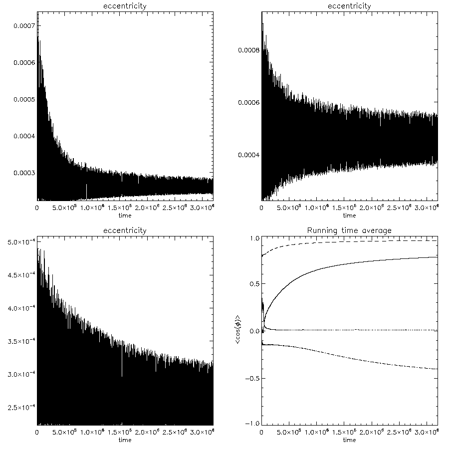
Figure 1: Time dependent evolution for Q’=10 and minimum masses. Shown is the eccentricity of the innermost planet (upper left panel), middle planet (upper right panel) and outermost planet (lower right panel) as a function of time. Running time averages of the cosines of the resonant angles are shown in the lower right panel. These correspond to $\Phi_{1}=2\lambda_{2}-\lambda_{1}-\varpi_{1}$(full line), $\Phi_{2}=2\lambda_{2}-\lambda_{1}-\varpi_{2}$( dotted line), $\Phi_{3}=2\lambda_{3}-\lambda_{2}-\varpi_{2}$(dashed line), $\Phi_{4}=2\lambda_{3}-\lambda_{2}-\varpi_{3}$( dot dashed line). For all plots time is measured in yr.

We have also investigated the dependence of the evolution on $Q^{\prime},$ small variations of the initial semi-major axes and the magnitudes of the planet masses. Figure 2 shows the evolution for $Q^{\prime}=1000$, minimum masses and the initial innermost semimajor axis adjusted to make the innermost period ratio 2.23. In this case, the mean values of the eccentricities show evidence only of limited evolution. Nonetheless, running time averages of the cosines of $\Phi_{1}$ $\Phi_{3}$ and $\Phi_{4}$ quickly attain steady non zero values. This is consistent with the evolution of these runs being driven by tidal effects and towards a resonant state in which the resonant angles are associated with secular evolution of the orbital elements. This is able to occur without precise commensurability only because the eccentricities are very small (see appendix A). For comparison in Fig. 3 we plot the running means of $e_{1}\cos\Phi_{1},$ $e_{2}\cos\Phi_{3},$ and $e_{3}\cos\Phi_{4}$ for the same run. These also attain non zero values also indicating long term variations associated with the corresponding resonant angles. Note that the cosines of the resonant angles are not special in this respect (see also appendix A).

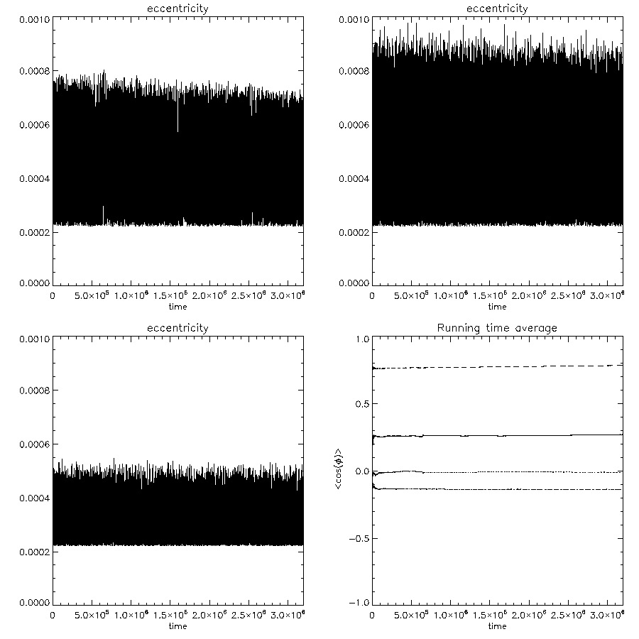
Figure 2: As in Fig.1 but for $Q^{\prime}=1000$, minimum masses and initial innermost period ratio 2.23.

The dependence on the planet mass scale is illustrated in Fig. 4 which shows the evolution for $Q^{\prime}=10$, twice the minimum masses and without adjustment of the innermost semi-major axis. Figure 5 gives the evolution for the same system but with the initial innermost semimajor axis adjusted to make the innermost period ratio 2.23. Both these runs show similar evolution to the minimum mass case illustrated in Fig. 1 but scaled to larger eccentricities. Thus the results are not sensitive to the choice of minimum masses or small changes in the semi-major axes.

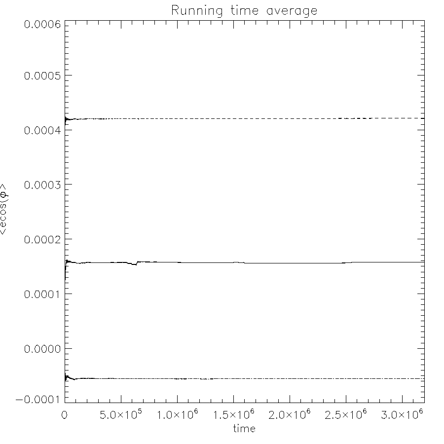
Figure 3: Evolution of the running time averages of $e_{1}\cos\Phi_{1}$ (solid line) $e_{2}\cos\Phi_{3}$ (dashed line) and $e_{3}\cos\Phi_{4}$ (dot-dashed line) for Q’=1000 and minimum masses. Time is measured in yr.

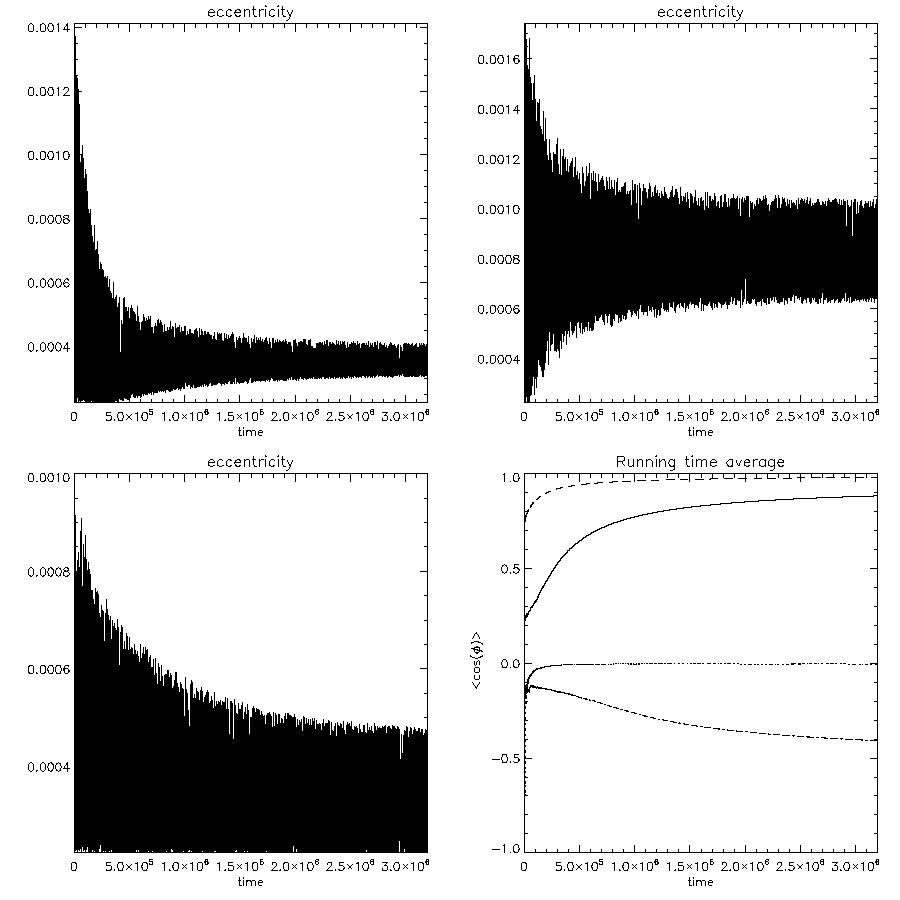
Figure 4: As in Fig.1 but with Q’=10 and with masses a factor of two larger than the minimum.

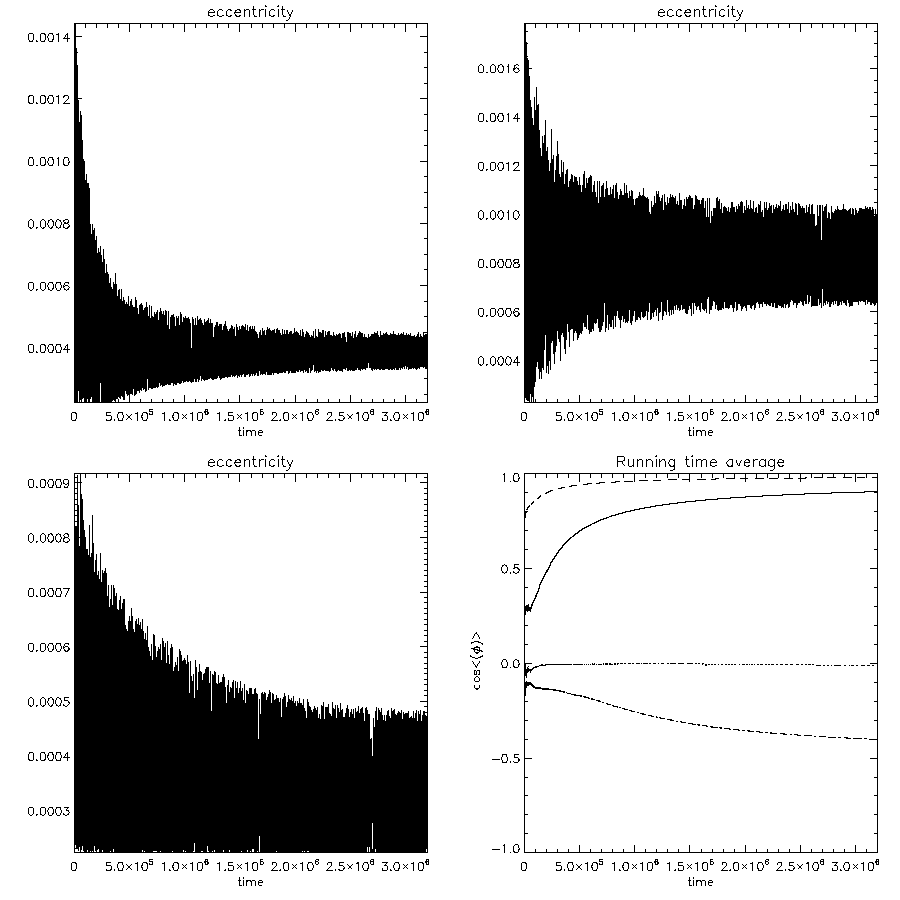
Figure 5: As in Fig.4 but with initial inner period ratio 2.23.

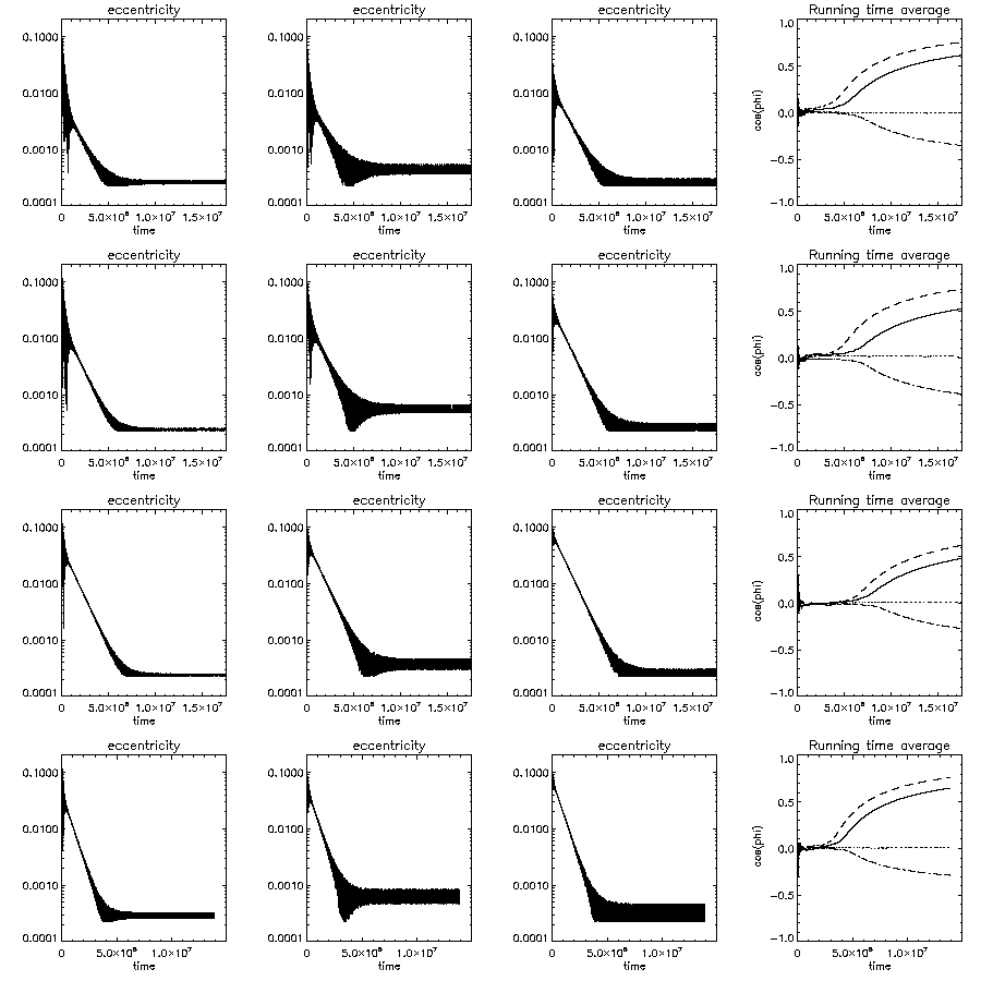
Figure 6: The evolution of the eccentricities and running time averages of the resonant angles are plotted as functions of time measured in years for simulations with $Q^{\prime}=10.$ The first second and third rows of panels correspond to the cases where the inner, middle and outer planets were started with an initial eccentricity (see text) respectively and minimum masses were adopted. The fourth row is the same as the third except that the planet masses were twice the minimum values. From left to right for each row, the first panel shows the eccentricity of the innermost planet, the second the eccentricity of the middle planet and the third panel shows the eccentricity of the outermost planet. The fourth panel shows running time averages of $\cos(\Phi_{1})$ (solid line), $\cos(\Phi_{2})$ (dotted line) $\cos(\Phi_{3})$ (dashed line) and $\cos(\Phi_{4})$ (dot-dashed line).

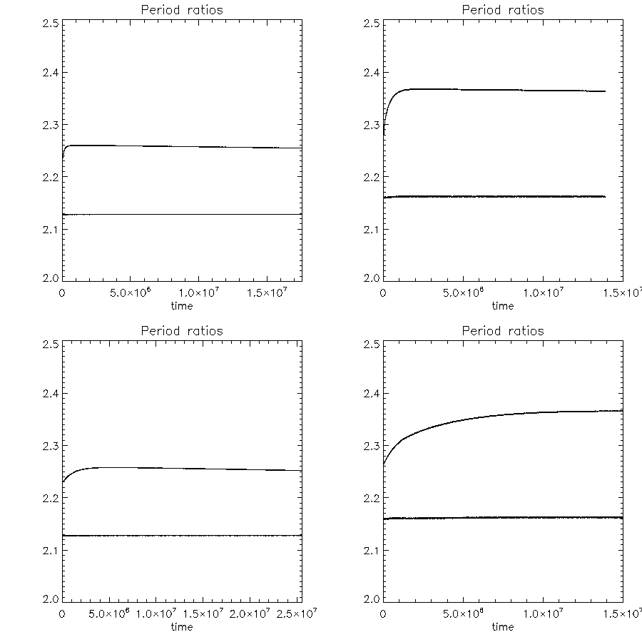
Figure 7: Evolution of the period ratios. The upper curve in each panel corresponds to the period ratio of the inner pair of planets and the lower curve to the period ratio of the outer planets. The upper left panel corresponds to minimum masses, $Q^{\prime}=10$ and the innermost planet was started with a non zero eccentricity (see text). In the upper right panel the masses were twice the minimum values, $Q^{\prime}=10$ and the outermost planet was started with a non zero eccentricity. The lower left panel was as for the upper left panel but $Q^{\prime}=100.$ The lower right panel was as for the upper right panel but $Q^{\prime}=100.$ Time is measured in yr. Note that the shifts occurring in the period ratios are independent of $Q^{\prime}.$

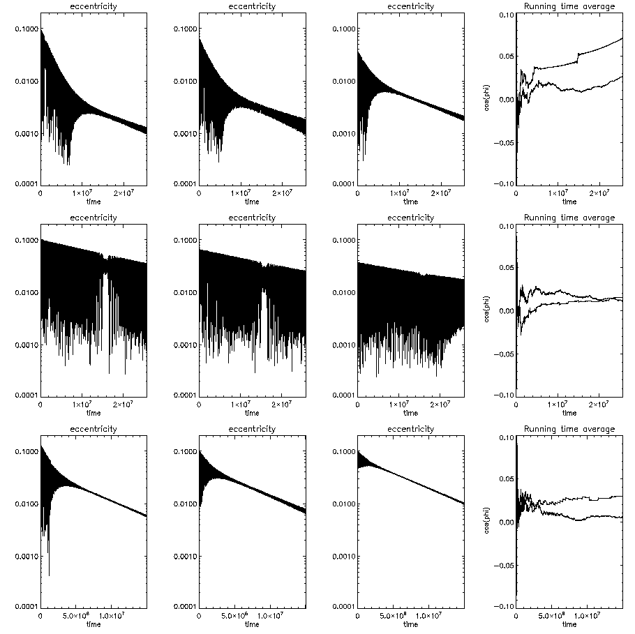
Figure 8: The evolution of the eccentricities and running time averages of the cosines of the resonant angles are plotted as functions of time measured in years. For the first and second rows of panels, $Q^{\prime}=100$ and $Q^{\prime}=1000$ respectively, minimum masses were adopted and the innermost planet was started with a non zero eccentricity (see text). For the fourth $Q^{\prime}=100$ and the masses were twice the minimum values. In this case the outermost planet was started with a non zero eccentricity. From left to right for each row, the first panel shows the eccentricity of the innermost planet, the second the eccentricity of the middle planet and the third panel shows the eccentricity of the outermost planet. The fourth panel shows running time averages of $\cos(\Phi_{1})$ and $\cos(\Phi_{3})$ (ultimately uppermost).

3.1 The effect of initial eccentricity

The calculations described above started with the planets on circular orbits. The motivation for this is that it is expected that tidal circularization will lead to a state closely approaching this provided that initial eccentricities are not so large as to disrupt the system. In order to explore this aspect in more detail, we have carried out a number of simulations which started with non circular orbits. We have explored initial eccentricities $\leq\sim 0.1$ and found that the system enters into an eccentricity decay mode that causes the system to evolve towards the state we found starting from circular orbits in which three of the resonant angles move towards libration with non zero values for the running time averages of their cosines.

In order to illustrate this we describe here results obtained when just one of the planets was started with a non zero eccentricity for various values of $Q^{\prime}\leq 1000.$ To initiate the system it was started as for the simulation illustrated in Figure 1 but with one of the planets set at pericentre in an orbit with the same angular momentum but with an eccentricity $e_{imp}\sim 0.1.$ This is equivalent to transfer to a less tightly bound orbit with the original specific angular momentum, but with the specific energy multiplied by $1-e_{imp}^{2}.$ In all cases the eccentricities of the planets become coupled and start to decay. After a while the system attains a slow decay mode for which, in a time average sense, the eccentricities are in an approximately constant ratio such that $e_{2}/e_{1}\sim 1.2$ and $e_{3}/e_{1}\sim 1.6.$

Fig. 6 illustrates the evolution of the eccentricities and running time averages of the cosines of the resonant angles for minimum mass simulations with $Q^{\prime}=10.$ Cases for which the innermost, middle and outermost planet respectively had an initial eccentricity are shown. For comparison a case with twice the minimum masses and for which the outermost planet was started with a non zero eccentricity is also shown. The evolution of all of these systems was as described above.

However, the introduction of the initial eccentricity while conserving the angular momentum of the system causes the semi-major axes and hence the period ratios in the system to change. This evolution involves energy dissipation at fixed angular momentum and thus the system must spread radially as for an accretion disc (eg. Lynden-Bell & Pringle 1974). This causes the period ratios to increase (see Fig. 7). When this happens the system attains period ratios that differ from the original ones. However, this is easily compensated for by starting with appropriately shifted initial conditions. The important point is that we get the same type of evolution independently of such shifts. Fig. 7 shows that the largest shift occurs when the outermost planet starts with an initial eccentricity. The period ratio of the innermost pair shifts from $2.23$ to $2.37.$ A consequence of this is that the forced eccentricity of the innermost planet is $\sim 25\%$ smaller in this case than in the case where the inner planet started with a non zero eccentricity (see Fig. 6). We remark that the same evolution is obtained when the masses are increased by a factor of two except that the ultimate eccentricities are a factor between $1.5$ and $2$ larger. The above trends are in qualitative agreement with a simplified discussion of the resonant interaction between the planets that we give in appendix A even though only two of the resonant angles $\Phi_{1}$ and $\Phi_{3}$ are found to be librating at this point with $\cos(\Phi_{4})$ having a non zero time average of relatively small magnitude.

Finally we have checked that changing $Q^{\prime}$ gives the same form of solution but with an evolutionary time that scales with $Q^{\prime}.$ Results for $Q^{\prime}=100$ and $Q^{\prime}=1000$ that confirm this view when compared with results already described for $Q^{\prime}=10$ are illustrated in Fig. 8. However, practical considerations mean that runs with large $Q^{\prime}$ cannot be followed to libration of the resonant angles. Nonetheless when $Q^{\prime}=100,$ $\cos(\Phi_{3})$ and $\cos(\Phi_{1})$ begin to attain non zero running means at the end of simulations with minimum masses after $2.5\times 10^{7}yr.$ This indicates that resonance could be effectively entered for $Q^{\prime}<10^{4}$ within the lifetime of such systems. These results taken together suggest that the planets may be undergoing circularization in a three planet resonance.

As the circularization process involves energy dissipation at fixed angular momentum, the system must spread increasing the period ratios of neighbouring planets. Although this means an increasing departure from strict commensurability, resonant angles remain librating or circulating in such a way as to enable the required redistribution of angular momentum to take place. A simple model illustrating how this works is given in appendix A. The amount of spreading and increase in the period ratios that can take place in a given time depends on $Q^{\prime}.$ We investigate this in the context of a migration scenario for producing the configuration below.

Simulations incorporating migration indicate that the planets were likely to have been in a strict Laplace resonance with all four angles librating. However, if this persists the period ratios would increase maintaining a larger departure from commensurability for the outer pair than the inner pair in disagreement with observations. Thus some perturbation event must have disrupted this resonance enabling the planets to continue circularizing with the correct period ratio relationships. As we have seen above, giving one of the planets a relatively small eccentricity can produce significant changes to the period ratios.

To investigate this scenario, we now describe simulations of systems of three planets migrating inwards in a disc that set up a Laplace resonance. We go on to study the evolution following from its disruption as the result of a perturbation applied once the planets have decoupled from the disc.

4 Migration and interaction with the star: Simulation results

In all the runs we have performed, the planets converge on each other forming a three planet 4:2:1 resonance, and migrate in locked in that configuration. Whether the resonance can be maintained all the way down to the disc inner cavity depends on how fast the migration is. There is a tendency for the 4:2:1 resonance to be stable for slow migration rates but to be disrupted, with the appearance of higher order resonances once the migration rate becomes sufficiently fast. However, the evolution is difficult to predict precisely, as the transition from the 4:2:1 resonance to higher order resonances happens through an instability which appears to be extended in time and chaotic. Small changes to the model parameters in this regime may affect whether this instability occurs or not within a given time interval. Similar phenomena have been seen in two planet resonant migration where a sequence of resonances can be formed, maintained and subsequently disrupted in turn (see Papaloizou & Szuszkiewicz 2009).

Figure 9 shows the evolution of the semi–major axes of the planets and of the period ratios for 3 planets with minimum masses initially located at 0.2, 0.34 and 0.6 au, respectively. The disc aspect ratio is $H/r=0.05.$ Equations (6) and (7) for the migration and circularization times are used with $M_{d}=2.5\times 10^{-5}$ M${}_{\odot}.$ This was equal to the disc mass within 5 au in the original formalism of Papaloizou & Larwood (2000). However, as there is much uncertainty in the migration rates to be used for low mass planets we investigate different possibilities using this parameter to scale the migration and circularization rates (see section 2.2). Used in this way it no longer corresponds to a disc mass as in the original formulation.

The initial migration times for this case are then $2.8\times 10^{5}$ and $4\times 10^{5}$ years for the innermost and outermost planets respectively. The initial period ratios for the inner and outer pairs are $2.21$ and $2.34$, respectively. This calculation led to the setting up of a Laplace resonance that is maintained during the subsequent evolution of the system, although for a finite period of a time around $2\times 10^{6}$ years a temporary weak and inconsequential instability was present (see below).

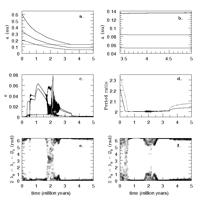
Figure 9: Semi–major axis $a$ (in au, plots a and b), eccentricity $e$ (plot c), period ratios (plot d), resonant angles $\Phi_{1}=2\lambda_{2}-\lambda_{1}-\tilde{\omega}_{1}$ (in rad., plot e) and $\Phi_{3}=2\lambda_{3}-\lambda_{2}-\tilde{\omega}_{2}$ (in rad., plot f) versus time (in million years) for 3 planets initially located at 0.2, 0.34 and 0.6 au. On plots a and b, each solid line represents a planet, whereas the dotted line indicates the location of the disc inner edge. Note the different time interval for plot b. On plot c, the solid and dotted lines represent the period ratio of the inner and outer pair of planets, respectively. Here $M_{d}=2.5\times 10^{-5}$ M_⊙ and $Q^{\prime}=10^{-2}$ (note that the evolution during the disc migration phase is not sensitive to the value of this parameter). Even though strict commensurability is lost as a result of tidal interaction with the star, the planets stay locked in resonances, as indicated by the behaviour of the resonant angles.

In these calculations , the tidal $Q^{\prime}$ parameter was set to $10^{-2}$. This is at least 3 orders or magnitude smaller than the values supposed to apply in Earth–like planets, but this value was chosen to give evolutionary timescales that could be reasonably handled numerically (i.e. runs that could be done within weeks on a single processor). Tests carried out below with more realistic values of $Q^{\prime}$ indicate that the evolution during the disc migration phase is not affected by this specification. Furthermore, when the planets are inside the cavity, the scaling given by equation (47) holds, implying that increasing $Q^{\prime}$ corresponds to scaling to a longer evolutionary timescale. With $Q^{\prime}=10^{-2}$, the eccentricity damping timescale given by equation (5) is $t_{e,i}^{s}=400$ years for a 1 M_⊕ planet at 0.05 au, inducing a timescale on which the semi–major axis evolves of about $2\times 10^{8}$ years for an eccentricity of $10^{-3}$ (see section 2.1).

Figure 9 shows the evolution of the semi–major axes, the eccentricities, the period ratios and the resonant angles $\Phi_{1}=2\lambda_{2}-\lambda_{1}-\tilde{\omega}_{1}$ and $\Phi_{3}=2\lambda_{3}-\lambda_{2}-\tilde{\omega}_{2}$. As pointed out above, the Laplace resonance for which all four resonant angles librate is established while the planets migrate in the disc, after about $5\times 10^{5}$ years. The resonant angles $\Phi_{1}$ and $\Phi_{3}$ stay close to zero. Then, while some of the planets are still in the disc, a weak instability appears for a finite period of time (after about $2\times 10^{6}$  years) and the resonance is weakened with the angles driven to large amplitude libration with an occasional circulation. But the instability eventually dies out and the resonance is recovered before the planets decouple from the disc. Note that this instability is not always seen in the runs we have performed. As indicated above it seems to be associated with an approach to a transition to a resonance of higher degree. This is indicated by the fact that when the migration rate was speeded up by a factor of $4,$ the outer pair of planets underwent a transition to a $3:2$ resonance while the inner pair maintained a $2:1$ commensurability at the point at which the semi-major axes had attained the same configuration.

During the migration phase, the eccentricities are pumped up to several hundredths. Because of the low value of $Q^{\prime}$, tidal interaction with the star begins to affect the evolution of the system slightly before the outermost planet penetrates inside the cavity. Once the outermost planet reaches the disc inner edge, the disc is removed altogether from the calculation, so that if the planet is pushed out again it will not interact with the disc. This procedure is introduced to take into account the disappearance of the disc on a timescale of a few million years. In this particular run, the outermost planet enters the cavity after $3.5\times 10^{6}$ years. At that point, changes in semi–major axes are due only to tidal interaction with the star. As the eccentricities of the two inner planets are damped from a few $10^{-3}$ to $10^{-3}$, their semi–major axes decrease by about 1 percent (see plot b of fig. 9) in such a way that their period ratio increases by somewhat more than a percent, going from 2 to 2.037 (see plot d of fig. 9).

In the meantime, the eccentricity of the outermost planet is hardly affected, as it was already very small (a few $\times 10^{-4}$) when the planet entered the cavity. Because of the conservation of the total angular momentum though, its semi–major axis increases by about 1 percent, which results in the period ratio of the outer pair of planets increasing by a few percent, from 2 to 2.077. Therefore, strict commensurability is lost. However, we note that the resonant angles still librate, so that the Laplace resonance is not disrupted. The fact that the deviation of the outer period ratio from 2 is twice the deviation of the inner period ratio from 2 is a consequence of the Laplace relation (equation [38] of appendix A) and this feature is preserved in the subsequent evolution of this and similar cases. As we shall see, these deviations increase approximately $\propto t^{1/3}$, as predicted from equation (47).

As noted above, the Laplace relation is not satisfied in HD 40307. As we shall see below, it is possible to obtain the correct relationship between the period ratios provided the Laplace resonance is disrupted such that only $\Phi_{1},\Phi_{3}$ and $\Phi_{4}$ librate and contribute to the secular evolution (see also section 3.1) .

In order to investigate the dependence on the specification of the circularization rates induced by the disc, we have performed simulations for which these depend only on the planet mass and are therefore constant. We here consider examples for which:

$$t_{m,i}=7\times 10^{6}\;\frac{{\rm M}_{\oplus}}{m_{i}}\;\;{\rm yr},$$ (8)

and:

$$t_{e,i}^{d}=8\times 10^{3}\;\frac{{\rm M}_{\oplus}}{m_{i}}\;\;{\rm yr}.$$ (9)

Results for cases both with the minimum masses for HD 40307 and twice the mimimum masses are plotted in Figure 10. During the disc induced migration, a three planet resonance is formed in both cases. As expected, the evolution for the higher mass case is twice as fast but otherwise similar. The resonance shows only small signs of instability while the planets migrate inwards. This is probably helped by the fact that the migration rate is here constant rather than increasing inwards as in the previous simulation. As the migration continues, the resonant angles $\Phi_{i}$ ($i=1,...,4$) all enter libration, but after the planets enter the cavity there is an adjustment so that only $\Phi_{1}$ and $\Phi_{3}$ librate. The system then evolves back towards a Laplace resonance where all angles librate or contribute to long term time averages. This latter aspect is similar to what was seen in the simulations with larger $Q^{\prime}$ illustrated in Figs. 1–5.

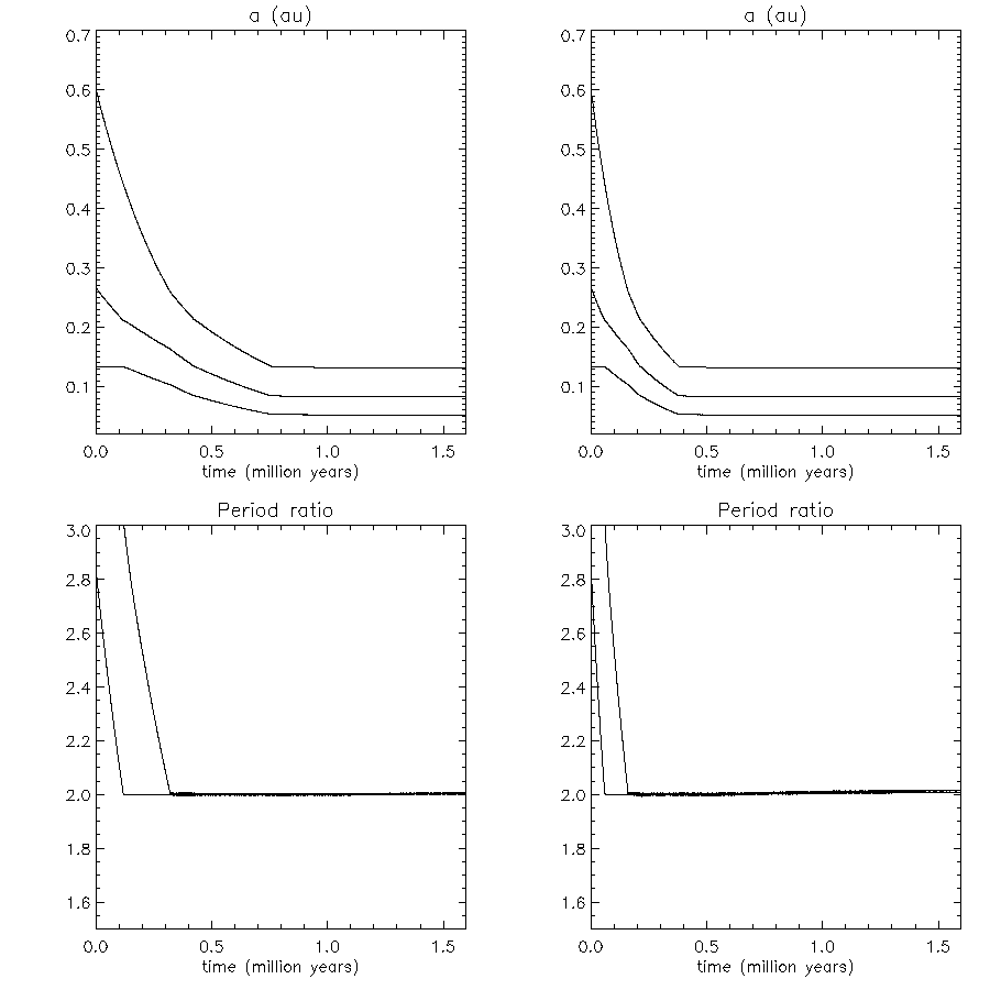
Figure 10: The evolution of model systems with the minimum masses of HD 40307 (left panels) and twice the minimum masses (right panels) showing the formation and maintenance of three planet resonance as a result of disc migration. For these models, the migration and circularization rates are constant and $Q^{\prime}=10$ (although evolution during the disc migration phase is not sensitive to this parameter)

. The upper panels give the evolution of the semi–major axes and the lower panels the period ratios.

This final evolution is one where the eccentricities all reduce and the planets physically separate with increasing period ratios for the inner and outer pairs of planets. This form of evolution is to be expected in a Keplerian system in which energy is dissipated while the total angular momentum is conserved, as is the case for an accretion disc (e.g., Lynden–Bell and Pringle 1974). It is this form of evolution we investigate below and how far the tidal effects of circularization can bring the system towards the HD 40307 system.

4.1 Disruption of the resonance

As the continuation of the simulations described above maintains a three planet Laplace resonance, the period ratios will not have the same form as in HD 40307. As indicated above the system has a larger period ratio for the inner pair as compared to the outer pair whereas the Laplace relation leads to the converse. However, we have found that there are resonant interactions for which only $\Phi_{1},\Phi_{3},$ and $\Phi_{4}$ librate. Hereafter we refer to this as the standard state of libration. This can lead to the required form for the period ratios but some disruption of the form of the resonance initially set up within the cavity needs to take place. Mechanisms could involve close encounters or collisions occurring shortly after the disc migration phase.

We comment that we have found it impossible to disrupt the 2:1 resonance of the inner pair of planets with a slow process. For instance, we have added a fourth planet on an inclined orbit, but found that even a massive perturber (3 Jupiter masses) at 5 au could not take the inner pair away from the 2:1 resonance. To do this, the parameters of one or more of the orbits have to be varied suddenly preventing the resonance from responding adiabatically. An encounter with a fourth planet on a parabolic orbit is a possible means to achieve this and there are other possibilities involving one or more direct collisions. To affect the resonance, the semi–major axis of one of the planets should change by more than an effective libration width associated with one of the resonant angles. We have performed simulations for which the velocity components of one of the planets were all suddenly increased or decreased by a constant factor. This has the effect of preserving circular orbits which is reasonable under conditions of effective circularization. We found that fractional changes exceeding $\sim 2\times 10^{-3}$ were sufficient and, provided the changes were not too excessive, simulations approach the same form of evolution.

Below we describe a simulation where an impulsive change that decreased the velocity components of the innermost planet by $0.996$ was applied just after the outermost planet entered the cavity. The end of the simulation illustrated in Fig. 10 (or its larger planet mass counterpart where appropriate) was used as a starting point for the simulations presented below, as these are reasonable outcomes for a system having undergone inward migration induced by a disc and then entered an inner cavity. In some cases, the tidal parameter $Q^{\prime}$ was also adjusted.

We remark that we have performed simulations with other types of applied impulse. For example we have augmented the above form by giving the innermost planet an initial eccentricity in a similar manner to that undertaken in section 3.1. When this is small and typically of order $10^{-3}$ this makes no difference on account of rapid effective circularization. We have also considered impulsive changes to the outermost planet giving it an eccentricity $\sim 0.1$ as in section 3.1. In this case period ratios can be shifted to be close to the observed ones just after the outermost planet has entered the cavity (see below).

4.2 Evolution of systems on three planet resonances undergoing circularization and radial spreading

In Fig. 11, we illustrate the evolution of a model system of three planets with masses twice the minimum masses of HD 40307 with $Q^{\prime}=10.$ Two runs are displayed. The first one continues the evolution of the corresponding case plotted in Fig. 10. In the second run, an impulse was first applied to the innermost planet that reduced all velocities by a factor of $0.996.$

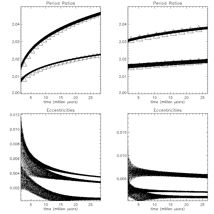
Figure 11: Evolution of a model system of three planets with masses twice the minimum masses of HD 40307. The left panels correspond to a continuation of the evolution from the corresponding case illustrated in Fig. 10. The right panels correspond to the evolution after an impulse was applied to the inner planet (see text). For both models $Q^{\prime}=10.$ The period ratios $n_{1}/n_{2}$ and $n_{2}/n_{3}$ are plotted as a function of time in the upper panels. The upper curve corresponds to the outer pair (left panel) and the inner pair (right panel). In this and similar figures below, the triangles correspond to analytic fits of the form given by equation 10) (and see text). The lower panels show the evolution of the eccentricities of the three planets. In the lower left panel the curves from top down correspond to the inner, middle and outer planets respectively. In the lower right panel the curves from top down correspond to the middle, lower and outer planet.

As shown in Fig. 11, during the subsequent evolution the system spreads radially with increasing period ratios. The way this happens is illustrated by the simple model described in appendix A. In this discussion the period ratios are replaced by the quantities $W_{1,2}=n_{1}/n_{2}-2$ and $W_{2,3}=n_{2}/n_{3}-2$ that are easily obtained from Fig. 11. We have been able to find good fits to the time evolution of the form found in appendix A as given by equation (47)

$$W_{i,i+1}=\left(\frac{t_{6}-\beta}{\alpha}\right)^{1/3},\;\;\;i=1,2,$$ (10)

where $\alpha$ and $\beta$ are constants and $t_{6}$ is the time in units of $10^{6}$ yr measured from the start of the relevant simulation shown in Fig. 10.

In the case with no initial impulse, $\alpha=2.77\times 10^{5}$ and $\beta=1.5$ for the outer pair, and $\alpha=2.37\times 10^{6}$ and $\beta=$1.5 for the inner pair. For the case with an initial impulse, $\alpha=7.73\times 10^{6}$ and $\beta=-26.5$ for the outer pair, and $\alpha=9.66\times 10^{5}$ and $\beta=-26.5$ for the inner pair. For the latter case, a standard libration state occurred with the deviation of the inner period ratio from two being about a factor of two larger than the corresponding deviation for the outer period ratio, similar to the situation in HD 40307. This is in contrast to the case with no impulse that persisted in a Laplace resonance with all angles librating. In that case, the Laplace relation persists which leads to the relative deviation of the period ratios from two behaving differently from HD 40307 (see above).

Despite this, we can estimate the time it would take to obtain the outer period ratio of 2.13 appropriate to HD 40307. This is $6.1\times 10^{8}$ yr. The scaling of the circularization time, $t_{e,i}^{s}\propto m_{i}^{-2/3}$ leading to the scaling of the evolution time, $t,$ to reach a given state, with mass of the form $t\propto m_{i}^{-8/3},$ implies that for a minimum mass system this would be $\sim 4\times 10^{9}$ yr. Thus, it might just be possible to achieve the outer period ratio in this case but then the inner period ratio would have to be determined subsequently by alternative means.

For the case with the applied impulse, we may estimate the time to bring the inner period ratio to the appropriate value $2.23.$ This is somewhat uncertain because of the small variation seen in the simulation, but it is about $\sim 1.1\times 10^{10}$ yr. Note that the relative period ratios are not precisely identical to those of HD 40307. In particular the ratio of the deviation of the inner period ratio from two and, the deviation of the outer period ratio from two is about $30\%$ too large. However, this may be adjusted by changing simulation input parameters. For example we recall that the simulations reported here were performed with the same value of $Q^{\prime}$ for all of the planets. To indicate one possibility we note that tests we have performed indicate that the above ratio may be reduced by taking a smaller value of $Q^{\prime}$ for the outermost planet than the others.

We remark that, while it might be barely possible to obtain an inner period ratio of 2.23 for a larger mass system, it is almost certainly not possible for the minimum mass system as the time required would be $\sim 6.98\times 10^{10}$ yr.

Note that, as the evolution progresses, the eccentricities of all the planets tend to decrease, as does their variation. This is a general consequence of the spreading that is driven by the energy dissipation in these simulations.

To investigate further the form of the evolution and its scaling with run parameters, we plot in Fig. 12 the results of two simulations of models with minimum masses and for which an impulse of the above form was applied to the innermost planet. We compare cases with $Q^{\prime}=0.01$ and $Q^{\prime}=0.1.$ As stated above, we had to consider rather small values in order to perform simulations that produced a reasonable variation in a reasonable time. These resulted in a standard state of libration and relative period ratios very similar to the higher mass simulation with an initial impulse illustrated in Fig. 11.

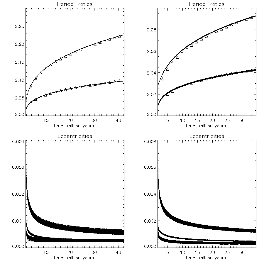
Figure 12: As in Fig. 11, but for models with minimum masses and for which an impulse was applied to the innermost planet (see text). For the left panels, $Q^{\prime}=0.01$ and for the right panels, $Q^{\prime}=0.1.$ In the upper panels, the upper curves correspond to the inner period ratio. In the lower panels, the curves from top down correspond to the middle, inner and outer planets respectively.

In the case with $Q^{\prime}=0.01$, the fit parameters are $\alpha=3.58\times 10^{3}$ and $\beta=1.7$ for the inner pair, and $\alpha=4.20\times 10^{4}$ and $\beta=$1.7 for the outer pair. For the case with $Q^{\prime}=0.1$, they are $\alpha=4.13\times 10^{4}$ and $\beta=1.5.$ for the inner pair, and $\alpha=4.18\times 10^{5}$ and $\beta=$1.5 for the outer pair. The values of $\alpha$, being about an order of magnitude larger in the second case, are consistent with the evolution time being an order of magnitude larger, thus scaling with $Q^{\prime}$ as expected. The time to attain an inner period ratio of $2.23$ in the $Q^{\prime}=0.01$ case is $\sim 4.4\times 10^{7}$ yr, leading to an estimate of $\sim 4.4\times 10^{10}$ yr when $Q^{\prime}=10.$ This is less than the estimate based on the analytic scaling with planet mass implied by equation (47) applied to the higher mass simulations illustrated in Fig. 11 by a factor $\sim 1.5,$ which we believe is a reasonable level of consistency in view of the extent of the extrapolation involved. The eccentricities in these simulations decrease with time in a manner analogous to the simulations shown in Fig. 11.

The long times required for the above cases to reach a configuration similar to that now observed in HD 40307 arise because only a very small perturbation was applied just after the systems decoupled from the disc, requiring a large amount of subsequent period ratio evolution. Such a scenario is only feasible for masses exceeding twice the minimum and small $Q^{\prime}\sim 10.$

However, if a larger perturbation is allowed, it can provide a larger shift in the period ratios requiring less evolution later on (see Fig. 7). This is equivalent to starting on the evolutionary curves shown in Figs. 11-12 at a later time.

For example we found that if a perturbation of the type adopted in section 3.1 was applied to the outer planet a shift of the right type could be obtained. We found that when the imposed eccentricity of the outer planet was taken to be $0.15,$ the period ratios were shifted to very similar values to those in HD 40307. Thus if large enough perturbations are allowed, only a small amount of subsequent evolution may be needed.

5 Discussion and conclusion

In this paper, we have shown that the planets around the star HD 40307 could be undergoing a resonant interaction, despite departure of the period ratios from very precise commensurability. This is indicated by the fact that three of the four resonant angles librate or are associated with long term changes to the orbital elements. Note that such a resonant state can occur without exact commensurability only because the eccentricities are very small, which can be brought about as a result of tidal circularization from a state with initially higher eccentricities (see section 3.1). When this occurs in a system that starts from a near 2:1 commensurability, the difference of the period ratios from two then increases $\propto t^{1/3}.$

We propose that the planets in this system were in a strict Laplace resonance while they migrated through the disc, with all 4 resonant angles librating. Exact commensurability was then departed from as indicated above as a result of the tidal interaction with the star, which preserved libration of at least some of the resonant angles, after the planets entered the disc inner cavity. Because of the Laplace relation , the period ratios evolve in such a way that the ratio for the inner pair of planets is smaller than that of the outer pair of planets. The opposite is observed in HD 40307.

To get the appropriate form for the period ratios, some disruption of the resonance set up in the cavity needs to take place (this is in contrast to claims by Zhou 2009). A close encounter for instance might be a possible cause. An impulsive interaction would be sudden enough that the resonance would not respond adiabatically. If the velocity of the innermost planet is reduced by a factor 0.996 for instance, deviation of the inner period ratio from two gets twice as large as the corresponding deviation for the outer period ratio, while 3 of the 4 resonant angles still librate, similar to the situation in HD 40307, within the lifetime of the system.

However, we found that we could get a period ratio of 2.23 for the inner pair only if the masses are significantly larger than the minimum masses and tidal dissipation is possibly unrealistically effective. From the results obtained in section 4, when the Laplace resonance is disrupted at an early stage, we estimate that the deviation of the inner period ratio from two is approximately given as a function of time by $W_{1,2}\sim 0.23(0.157\tilde{m}_{1}^{8/3}t_{10}/Q^{\prime}_{10})^{1/3},$ where $Q^{\prime}_{10}=Q^{\prime}/10,$ $t_{10}=t/(10^{10}~{}{\rm yr})$ and $\tilde{m}_{1}=m_{1}/4.2~{}{\rm M}_{\oplus}$ ($m_{2}/m_{1}$ and $m_{3}/m_{1}$ are assumed fixed for the purposes of this discussion). Accordingly, to attain $W_{12}=0.23,$ we would require masses exceeding the minimum estimate by about a factor of two for $Q^{\prime}_{10}\sim 1.$

If the Laplace resonance is preserved, from the results obtained in section 4, we may also estimate that the deviation of the outer period ratio from two is approximately given as a function of time by $W_{1,2}\sim(2.6\tilde{m}_{1}^{8/3}t_{10}/Q^{\prime}_{10})^{1/3}$. Thus it may be possible to get a period ratio of 2.13 for the outer pair of planets with near to minimum masses in a reasonable time if $Q^{\prime}_{10}\sim 1$ for all the planets, but then the inner period ratio would be only $\sim 2.065.$ It would thus seem likely that additional stronger dynamical interactions are required to bring the system to its final state.

For example we found that if the outer planet was given an eccentricity $e_{3}\sim 0.15$ shortly after decoupling from the disc, period ratios similar to those observed in HD 40307 could be produced on a time scale of a few $\times 10^{6}yr.$ (see sections 3.1 and 4). Then, the work presented in this paper indicates that tidal circularization would continue through resonant interaction with the period ratios separating after these interactions are over.

Note that a similar type of scenario may apply to the system of planets around GJ 581, which is currently closer to exact commensurablilty than HD 40307. Indeed, different mean motion resonances can be established while the planets migrate within the disc, depending on the initial relative location of the planets and on the migration timescale. However, as it appears that this system may have been in higher order resonances than HD 40307, it is possible that these would have been broken completely as a result of circularization. We intend to present a study of GJ 581 in a forthcoming paper.

In a study of the tidal evolution of the system around HD 40307, Barnes et al. (2009) have concluded that the planets cannot be Earth–like. According to them, if it were the case, extrapolating back in time the tidal evolution of the eccentricities from current values (estimated from direct simulations of the observed system), the system would have been unstable. The work in this paper does not support such a conclusion. We note that Barnes et al. (2009) neglected the dynamical interactions between the planets, which clearly will have played a role if the current eccentricities are small because resonant interactions coupled with tidal effects have been associated with long term changes to the orbital elements.

The results reported in this paper indicate that resonances in multiple low mass–planet systems may play more of a role than currently claimed in the literature. Significant departure from exact mean motion resonance does not necessarily preclude a resonant state when, for example, tidal effects are important causing eccentricities to be small, as libration of some of the resonant angles in that case may still exist, and be associated with long term evolution of the orbital elements. Although the confirmation of resonance effects is problematic for small eccentricities, we expect that further detections and analysis of systems similar to HD 40307 will test the relevance of the scenarios explored in this paper.

Finally, we comment that, because of the rapid increase of the effectiveness of tidal interactions with decreasing orbital period, the dynamical interactions discussed here would be of much greater importance for systems in which the period of the innermost planet is significantly shorter than in the HD 40307 system. For example, we note that the planet CoRoT–7 b, which has a projected mass of 11.12 M_⊕, has a period of only 0.85 day (Léger et al. 2009). If this short period orbit is a result of migration, it is likely this planet was pushed inwards by a companion which would have been on a commensurable orbit (Terquem & Papaloizou 2007). We note in support of this idea that pre-main sequence stars typically have rotation periods of several days (Bouvier et al. 1993), which would imply that the disc inner cavity should extend well beyond the orbit of CoRoT–7 b if that were magnetically maintained. In that case, this planet could not have migrated so far inwards without being shepherded by a companion.

Appendix A Semi–analytic model for a system in a three planet resonance undergoing circularization

In this appendix we develop a semi–analytic model that shows how a two or three planet system undergoes radial spreading as a result of evolution driven by tidal circularization. The coupling between the planets occurs because resonant angles may librate or be associated with long term changes even though there may be significant deviations from exact commensurability. We begin with the system without tides which is Hamiltonian. Subsequently, we add the effects of tides.

A.1 Coordinate system

We adopt Jacobi coordinates (Sinclair 1975, Papaloizou & Szuszkiewicz 2005) for which the radius vector of planet $i,$ ${\bf r}_{i},$ is measured relative to the centre of mass of the system comprised of $M$ and all other planets interior to $i,$ for $i=1,2...,N$ with $N=3$ here and $i=1$ corresponding to the innermost planet. The Hamiltonian, correct to second order in the planetary masses, can be written in the form:

$$H = \sum_{i=1}^{3}\left({1\over 2}m_{i}|\dot{\bf r}_{i}|^{2}-{GM_{i}m_{i}\over|{\bf r}_{i}|}\right)$$ (11)

$$- \sum_{i=1}^{3}\sum_{j=i+1}^{3}Gm_{i}m_{j}\left({1\over|{\bf r}_{ij}|}-{{\bf r}_{i}\cdot{\bf r}_{j}\over|{\bf r}_{j}|^{3}}\right).$$

Here $M_{i}=M+m_{i}$ and ${\bf r}_{ij}={\bf r}_{i}-{\bf r}_{j}.$

The equations of motion for motion in a fixed plane, about a dominant central mass, may be written in the form (see, e.g., Papaloizou 2003, Papaloizou & Szuszkiewicz 2005):

$$\dot{E}_{i} = -n_{i}\frac{\partial H}{\partial\lambda_{i}}$$ (12)

$$\dot{L}_{i} = -\left(\frac{\partial H}{\partial\lambda_{i}}+\frac{\partial H}{\partial\varpi_{i}}\right)$$ (13)

$$\dot{\lambda}_{i} = \frac{\partial H}{\partial L_{i}}+n_{i}\frac{\partial H}{\partial E_{i}}$$ (14)

$$\dot{\varpi}_{i} = \frac{\partial H}{\partial L_{i}}.$$ (15)

Here the orbital angular momentum of planet $i$ which has reduced mass $m_{i}=m_{i0}M/(M+m_{i0}),$ with $m_{i0}$ being the actual mass, is $L_{i}$ and the orbital energy is $E_{i}.$ For motion around a central point mass $M$ we have:

$$L_{i} = m_{i}\sqrt{GM_{i}a_{i}(1-e_{i}^{2})},$$ (16)

$$E_{i} = -{{GM_{i}m_{i}}\over{2a_{i}}},$$ (17)

where $M_{i}=M+m_{i0},$ $a_{i}$ denotes the semi-major axis and $e_{i}$ the eccentricity of planet $i.$

The mean longitude of planet $i$ is $\lambda_{i}=n_{i}(t-t_{0i})+\varpi_{i},$ where $n_{i}=\sqrt{GM_{i}/a_{i}^{3}}$ is its mean motion, with $t_{0i}$ denoting its time of periastron passage and $\varpi_{i}$ the longitude of periastron. We remark that results valid for a two planet system, $i=1,2$, may be obtained by setting $m_{3}=0.$

The Hamiltonian may quite generally be expanded in a Fourier series involving linear combinations of the five angular differences $\varpi_{1}-\varpi_{2},$ $\varpi_{2}-\varpi_{3}$ and $\lambda_{i}-\varpi_{i},i=1,2,3.$

Here we are interested in the effects of two first order $2:1$ commensurabilities associated with the outer and inner pairs of planets. In this situation, we expect that any of the four angles $\Phi_{1}=2\lambda_{2}-\lambda_{1}-\varpi_{1},$ $\Phi_{2}=2\lambda_{2}-\lambda_{1}-\varpi_{2},$ $\Phi_{3}=2\lambda_{3}-\lambda_{2}-\varpi_{2}$ and $\Phi_{4}=2\lambda_{3}-\lambda_{2}-\varpi_{3}$ may be slowly varying. Following standard practice (see, e.g., Papaloizou 2003, Papaloizou & Szuszkiewicz 2005), only terms in the Fourier expansion involving linear combinations of $\Phi_{1},$ $\Phi_{2},$ $\Phi_{3}$ and $\Phi_{4}$ as argument are retained. Working in the limit of small eccentricities applicable here, only terms that are first order in the eccentricities need to be retained.

Expanding to first order in the eccentricities, the Hamiltonian may be written in the form:

$$H=E_{1}+E_{2}+E_{3}+H_{12}+H_{23},$$ (18)

where:

$$H_{ij}=-\frac{Gm_{i}m_{j}}{a_{j}}\left[e_{j}C_{i,j}\cos(\Phi_{i+j-1})-e_{i}D_{i,j}\cos(\Phi_{2i-1})\right],$$ (19)

with:

$$C_{i,j} = {1\over 2}\left(x_{i,j}{db^{1}_{1/2}(x)\over dx}\Biggl{|}_{x=x_{i,j}}\Biggr{.}+3b^{1}_{1/2}(x_{i,j})-4x_{i,j}\right),$$ (20)

$$D_{i,j} = {1\over 2}\left(x_{i,j}{db^{2}_{1/2}(x)\over dx}\Biggl{|}_{x=x_{i,j}}\Biggr{.}+4b^{2}_{1/2}(x_{i,j})\right).$$ (21)

Here $b^{p}_{1/2}(x)$ denotes the usual Laplace coefficient (e.g., Brouwer & Clemence 1961) with the argument $x_{i,j}=a_{i}/a_{j}.$

A.2 Behaviour near a resonance with disc tides incorporated

Using equations (12)–(15) together with equation (18) we may first obtain the equations of motion without the effect of circularization tides and then add this in. We obtain correct to lowest order in the eccentricities:

$$\frac{de_{1}}{dt} =\frac{m_{2}a_{1}n_{1}D_{12}}{a_{2}M_{1}}\sin\Phi_{1}-\frac{e_{1}}{t_{e,1}^{s}},$$ (22)

$$\!\!\!\!\!\!\!\!\!\!\!\frac{de_{2}}{dt} =-\frac{n_{2}}{M_{2}}\left(m_{1}C_{12}\sin\Phi_{2}-\frac{a_{2}}{a_{3}}m_{3}D_{23}\sin\Phi_{3}\right)-\frac{e_{2}}{t_{e,2}^{s}},$$ (23)

$$\!\!\!\!\!\!\!\!\!\!\frac{de_{3}}{dt} =-\frac{m_{2}n_{3}C_{23}}{M_{3}}\sin\Phi_{4}-\frac{e_{3}}{t_{e,3}^{s}},$$ (24)

$$\!\!\!\!\!\!\!\!\!\!\dot{n}_{1} =-\frac{3n_{1}^{2}m_{2}a_{1}}{M_{1}a_{2}}\left(C_{12}e_{2}\sin\Phi_{2}-D_{12}e_{1}\sin\Phi_{1}\right)+\frac{3n_{1}e_{1}^{2}}{t_{e,1}^{s}},$$ (25)

$$\!\!\!\!\!\!\!\!\!\!\dot{n}_{2} =\frac{6n_{2}^{2}m_{1}}{M_{2}}\left(C_{12}e_{2}\sin\Phi_{2}-D_{12}e_{1}\sin\Phi_{1}\right)$$

$$-\frac{3n_{2}^{2}m_{3}a_{2}}{M_{2}a_{3}}\left(C_{23}e_{3}\sin\Phi_{4}-D_{23}e_{2}\sin\Phi_{3}\right)+\frac{3n_{2}e_{2}^{2}}{t_{e,2}^{s}},$$ (26)

$$\dot{n}_{3} =\frac{6n_{3}^{2}m_{2}}{M_{3}}\left(C_{23}e_{3}\sin\Phi_{4}-D_{23}e_{2}\sin\Phi_{3}\right)+\frac{3n_{3}e_{3}^{2}}{t_{e,3}^{s}},$$ (27)

$$\!\!\!\!\!\!\!\!\!\!\dot{\Phi}_{1} =2n_{2}-n_{1}-\frac{1}{\sqrt{GM_{1}a_{1}}m_{1}e_{1}}\frac{\partial H_{12}}{\partial e_{1}}\Biggl{|}_{a_{1},a_{2},a_{3}}\Biggr{.},$$ (28)

$$\!\!\!\!\!\!\!\!\!\!\dot{\Phi}_{2} =2n_{2}-n_{1}-\frac{1}{\sqrt{GM_{2}a_{2}}m_{2}e_{2}}\frac{\partial(H_{12}+H_{23})}{\partial e_{2}}\Biggl{|}_{a_{1},a_{2},a_{3}}\Biggr{.},$$ (29)

$$\!\!\!\!\!\!\!\!\!\!\dot{\Phi}_{3} =2n_{3}-n_{2}-\frac{1}{\sqrt{GM_{2}a_{2}}m_{2}e_{2}}\frac{\partial(H_{12}+H_{23})}{\partial e_{2}}\Biggl{|}_{a_{1},a_{2},a_{3}}\Biggr{.},$$ (30)

$$\!\!\!\!\!\!\!\!\!\!\dot{\Phi}_{4} =2n_{3}-n_{2}-\frac{1}{\sqrt{GM_{3}a_{3}}m_{3}e_{3}}\frac{\partial H_{23}}{\partial e_{3}}\Biggl{|}_{a_{1},a_{2},a_{3}}\Biggr{.}.$$ (31)

The terms on the right hand sides involving the circularization times $t_{e,i}^{s}$ describe the effects arising from tides raised by the central mass on planet $i.$ The terms $\propto e_{i}^{2}/t_{e,i}^{s}$ in equations (25), (27) and (28) account for the orbital energy dissipation occurring as a result of circularization at the lowest order in $e_{i}$ for which it appears.

A.3 Energy and angular momentum conservation

In the absence of tides, the total energy $E\equiv H$ and angular momentum $L=L_{1}+L_{2}+L_{3}$ are conserved. When circularizing tides act, the total angular momentum is conserved but energy is lost according to:

$$\frac{dE}{dt}=\sum_{i=1}^{3}\frac{2e_{i}^{2}E_{i}}{t_{e,i}^{s}}.$$ (32)

A.4 Resonance tides and migration

When both pairs of planets $(1,2)$ and $(2,3)$ are in resonance, a three planet resonance is said to exist. It is convenient to perform a time average of equations (22)-(31) taken over a time long compared to both the characteristic orbital period and the libration period , but short enough compared to the tidal time scale (see eg. Sinclair 1975 for a discussion of this aspect). The angles $\Phi_{i}$ may be undergoing libration or circulation.

Equations (22)–(27) may be averaged directly, while equations (28)–(31) may be averaged directly for small amplitude librations or alternatively after multiplying them by quantities such as either, e.g., $\cos\Phi_{1},$ $\cos\Phi_{2},$ $\cos\Phi_{3}$ and $\cos\Phi_{4}$ or $e_{1}\cos\Phi_{1},$ $e_{2}\cos\Phi_{2},$ $e_{2}\cos\Phi_{3}$ and $e_{3}\cos\Phi_{4}$, respectively. The time averages of these quantities as well as $\sin\Phi_{i}$ and $e_{i}\sin\Phi_{i},$ $(i=1,2,3)$ are assumed to vary on the tidal time scale or longer. When these are non zero, long term changes to the orbital elements $a_{i}$ and $e_{i}$ may occur through planet-planet interactions even without tides. As illustrated in Figures 2 and 3, six of these quantities are found to exhibit steady long term time averages of the required type that are quickly established for a model of HD 40307 with assumed $Q^{\prime}=1000.$

As this averaging procedure results in equations of essentially the same form as the case where the participating resonant angles (defined to be those that are associated with non zero time averages) are assumed to have averages close to but not equal to zero or $\pi,$ while undergoing small amplitude librations, leading to the same scaling with physical parameters, but with an adjustment of numerical coefficients. For simplicity we restrict consideration to that case. Assuming small amplitude librations of all four angles, equations (28)–(31) give relations of the form:

$$2n_{2}-n_{1} = \frac{m_{2}n_{1}a_{1}D_{12}\cos\Phi_{1}}{e_{1}M_{1}a_{2}},$$ (33)

$$2n_{2}-n_{1} = \beta,$$ (34)

$$2n_{3}-n_{2} = \beta,$$ (35)

$$2n_{3}-n_{2} = -\frac{m_{2}n_{3}C_{23}\cos\Phi_{4}}{e_{3}M_{3}},$$ (36)

where:

$$\beta=\frac{m_{3}n_{2}a_{2}D_{23}\cos\Phi_{3}}{e_{2}a_{3}M_{2}}-\frac{m_{1}n_{2}C_{12}\cos\Phi_{2}}{e_{2}M_{2}}$$ (37)

and the $\Phi_{i}$ in the above can be set to either zero or $\pi.$

We note that, when all four angles participate, equations (34) and (35) imply the strict Laplace resonance relation

$$3n_{2}-2n_{3}-n_{1}=0.$$ (38)

However, simulations of HD 40307 indicate that only $\Phi_{1},\Phi_{3},$ and $\Phi_{4}$ participate. Thus equation (34) is absent and the strict Laplace relation does not hold. Indeed, this relation implies that ${\cal L}=(n_{1}/n_{2}-2)/(n_{2}/n_{3}-2)n_{2}/n_{3}$ should be unity. Being about $4$, the Laplace relation is not satisfied. When $\Phi_{2}$ does not participate and the Laplace relation does not hold, the quantity ${\cal L}$ is not constrained from the outset but is determined as a consequence of the initial conditions and following time dependent evolution.

Below, we consider the case when either all four angles contribute or only $\Phi_{1},\Phi_{3}$ and $\Phi_{4}$ contribute. We note that a similar discussion applies when only $\Phi_{1},\Phi_{2}$ and $\Phi_{3}$ participate that leads to the same conclusions ($e_{3}$ decays independently due to tides in that case and may be taken to be zero). In all cases, one can readily verify that the above system provides a complete set of equations for the time averages of the resonant angles and the orbital elements when the form of the tidal forces is specified.

However, we note that we can obtain the characteristic form and time scale of the evolution by considering the conservation energy given by (32) together with the constancy of the total angular momentum. To do this we begin, by noting that equations (33) and (36) provide equations for the mean motion ratios of the form:

$$\frac{n_{2}}{n_{1}}=f_{2,1}(\xi_{2,1})\ \ \ \ {\rm where}\ \ \ \ \xi_{2,1}=\frac{m_{2}\cos\Phi_{1}}{e_{1}M_{1}},$$ (39)

and:

$$\frac{n_{3}}{n_{2}}=f_{3,2}(\xi_{2,1})\ \ \ \ {\rm where}\ \ \ \ \xi_{3,2}=\frac{m_{2}\cos\Phi_{4}}{e_{3}M_{3}},$$ (40)

and $f_{2,1}$ and $f_{3,2}$ are defined implicitly through equations (33) and (36). In addition, equation (35) gives $e_{2}$ in terms of $e_{3}$, $\xi_{2,1}$ and $\xi_{3,2}$ in the form:

$$\frac{e_{2}}{e_{3}}=\frac{m_{3}M_{3}n_{2}a_{2}D_{2,3}\cos\Phi_{3}-m_{1}M_{3}n_{2}a_{3}C_{1,2}\cos\Phi_{2}}{m_{2}M_{2}n_{3}a_{3}C_{2,3}\cos\Phi_{4}}.$$ (41)

When $\cos\Phi_{2}$ has zero time average and so is replaced by zero, equation (34) does not hold and accordingly the Laplace relation also does not hold. We comment that $\xi_{2,1}$ and $\xi_{3,2}$ measure the deviation from strict commensurability of the corresponding mean motions and do not have to be small. For a system such as HD 40307 these are large, particularly in comparison comparison to the characteristic size of the eccentricities.

We remark that according to equations (33) - (36), other things remaining fixed, the eccentricities are proportional to the planet mass scale and, inversely proportional to the deviation from commensurability. The results presented in section 3.1 confirm these trends but with some deviation that is to be expected because all the relevant resonant angles, although contributing to the evolution, are not in a state of small amplitude libration in those simulations.

A.5 Energy and Angular momentum conservation

Replacing $M_{i}$ ($i=1,2,3$) by $M$ to simplify expressions without loss of content (as $M\gg m_{i}$), the total energy and angular momentum may be written, respectively, as:

$$E=-\frac{GMm_{1}}{2a_{1}}\left[1+\frac{m_{2}f_{2,1}^{2/3}}{m_{1}}+\frac{m_{3}(f_{3,2}f_{2,1})^{2/3}}{m_{1}}\right],$$ (42)

and:

$$L=m_{1}\sqrt{GMa_{1}}\left[1+\frac{m_{2}}{m_{1}f_{2,1}^{1/3}}+\frac{m_{3}}{m_{1}(f_{3,2}f_{2,1})^{1/3}}\right].$$ (43)

Here, we have neglected in $L$ terms proportional to the squares of the eccentricities as these can be shown to lead to small effects compared to those arising from the eccentricity dependence of $f_{2,1}$ and $f_{3,2}.$ We now use the above together with equation (32) to form the quantity $L^{-2}d(EL^{2})/dt=dE/dt+(2E/L)dL/dt$ and find that this is given by:

$$-\frac{GMm_{2}}{3a_{2}}\left(1+\frac{2E}{Ln_{2}}\right)\frac{{\dot{f}_{2,1}}}{f_{2,1}}-\frac{GMm_{3}}{3a_{3}}\left(1+\frac{2E}{Ln_{3}}\right)\left(\frac{{\dot{f}_{2,1}}}{f_{2,1}}+\frac{{\dot{f}_{3,2}}}{f_{3,2}}\right)=\sum_{i=1}^{3}\frac{2e_{i}^{2}E_{i}}{t_{e,i}^{s}}.$$ (44)

We may write equation (44) in terms of the deviations from commensurabiity: $W_{2,1}=n_{1}/n_{2}-2=f_{2,1}^{-1}-2$ and $W_{2,3}=n_{2}/n_{3}-2=f_{3,2}^{-1}-2$, obtaining:

$$\frac{GMm_{2}n_{2}}{3a_{2}n_{1}}\left(1+\frac{2E}{Ln_{2}}\right){\dot{W}_{2,1}}+\frac{GMm_{3}}{3a_{3}}\left(1+\frac{2E}{Ln_{3}}\right)\left(\frac{n_{2}}{n_{1}}{\dot{W}_{2,1}}+\frac{n_{3}}{n_{2}}{\dot{W}_{2,3}}\right)=\sum_{i=1}^{3}\frac{2e_{i}^{2}E_{i}}{t_{e,i}^{s}}.$$ (45)

In addition, the right hand side can be expressed in terms of $W_{1,2}$ and $W_{2,3}$ using equations (33)–(36) which give:

$$\sum_{i=1}^{3}\frac{2e_{i}^{2}E_{i}}{t_{e,i}^{s}}=\frac{Gm_{1}m_{2}^{2}n_{1}^{2}a_{1}D_{1.2}^{2}\cos^{2}\Phi_{1}}{W_{2,1}^{2}Mn_{2}^{2}a_{2}^{2}t_{e,1}^{s}}+\left[1+\left(\frac{e_{2}}{e_{3}}\right)^{2}\frac{E_{2}t_{e,3}^{s}}{E_{3}t_{e,2}^{s}}\right]\frac{Gm_{3}m_{2}^{2}n_{3}^{2}C_{2,3}^{2}\cos^{2}\Phi_{4}}{W_{2,3}^{2}Ma_{3}n_{3}^{2}t_{e,3}^{s}}.$$ (46)

We may now obtain characteristic form of the time evolution of the departure from strict commensurability. To do this, we may simply assume that $W_{2,1},$ $W_{2,3}$ are comparable, significantly less than unity and $\sim W_{0},$ say, as has been found numerically in general and must be at least approximately the case for a strict Laplace resonance for which $W_{2,3}=2W_{2,1}/(1-W_{2,1})$ (see equation [38]). In addition, we take the planet masses to be comparable and $\sim m.$ Then the characteristic evolution expected from equations (45) and (46) can be obtained from an equation of the form $dW_{0}/dt\sim(m/M)^{2}/(t_{c}W_{0}^{2}),$ where we take $t_{c}$ to be the shortest circularization time $t_{e,i}.$ Thus:

$$W_{0}\sim\left(\frac{m}{M}\right)^{2/3}\left(\frac{t-t_{0}}{3t_{c}}\right)^{1/3},$$ (47)

where $t_{0}$ specifies an arbitrary origin of time. We recall that (47) applies to a two planet system by appropriately setting $m_{3}=0$ as well as a three planet system. The time required to attain a departure $W_{0}$ is $t-t_{0}\sim 3W_{0}^{3}(M/m)^{2}t_{c}$. In general, this is very much longer than the characteristic circularization time.

References

- [2009] Barnes R., Jackson B., Raymond S. N., West A. A., Greenberg R., 2009, ApJ, 695, 1006
- [2005] Bonfils X., Forveille T., Delfosse X., et al. 2005, A&A, 443, L15
- [1993] Bouvier J., Cabrit S., Fernandez M., Martin E. L., Matthews J. M., 1993, A&A, 272, 176
- [1961] Brouwer D., Clemence G. M., 1961, Methods of celestial mechanics, New York: Academic Press
- [2005] Brunini A., Cionco R. G., 2005, Icarus, 177, 264
- [1966] Goldreich P., Soter S., 1966, Icarus, 5, 375
- [2007] Ivanov P. B., Papaloizou J. C. B., 2007, MNRAS, 376, 682
- [2008] Kennedy G. M., Kenyon S. J., 2008, ApJ, 682, 1264
- [2008] Léger A., Rouan D., Schneider J., et al., 2008, astro-ph/0908.0241
- [1974] Lynden–Bell D., Pringle J. E., 1974, MNRAS, 168, 603
- [2009] Mayor M., Bonfils X., Forveille T., et al. 2009a, astro-ph/0906.2780
- [2009] Mayor M., Udry S., Lovis C., et al. 2009b, A&A, 493, 639
- [1999] Murray C. D., Dermott S. F., 1999, Solar System Dynamics (CUP), p. 254–255
- [2003] Papaloizou J.C.B., 2003, Cel. Mech. and Dynam. Astron., 87, 53
- [2000] Papaloizou J. C. B., Larwood J. D., 2000, MNRAS, 315, 823
- [2005] Papaloizou J.C.B., Szuszkiewicz E., 2005, MNRAS, 363, 153
- [2009a] Papaloizou J.C.B., Szuszkiewicz E., 2009, astro-ph:0911.1554
- [2001] Papaloizou J.C.B., Terquem C., 2001, MNRAS, 325, 221
- [2006] Paardekooper S.–J, Mellema G., 2006, A&A, 459, L17
- [2006] Paardekooper S.–J, Papaloizou J. C. B., 2008, A&A, 485, 877
- [2006] Paardekooper S.–J, Papaloizou J. C. B., 2009, MNRAS, 394, 2283
- [1993] Press W. H., Teukolsky S. A., Vetterling W. T., Flannery B. P., 1993, Numerical Recipes in FORTRAN (CUP)
- [2008] Raymond S. N., Barnes R., Mandell A. M., 2008, MNRAS, 384, 663
- [2009] Schlaufman, K. C., Lin, D. N. C., Ida S., 2009, Apj, .691, 1322
- [1975] Sinclair A. T., 1975, MNRAS, 171, 59
- [2002] Tanaka H., Takeuchi T., Ward W. R., 2002, ApJ, 565, 1257
- [2007] Terquem C., Papaloizou J. C. B., 2007, ApJ, 654, 1110
- [2007] Udry S., Bonfils X., Delfosse X., et al. 2007, A&A, 469, L43
- [1997] Ward W. R., 1997, Icarus, 126, 261
- [2009] Zhou J.–L., 2009, astro-ph/0902.4086