Localization, anomalous diffusion and slow relaxations: a random distance matrix approach

Abstract

We study the spectral properties of a class of random matrices where the matrix elements depend exponentially on the distance between uniformly and randomly distributed points. This model arises naturally in various physical contexts, such as the diffusion of particles, slow relaxations in glasses, and scalar phonon localization. Using a combination of a renormalization group procedure and a direct moment calculation, we find the eigenvalue distribution density (i.e., the spectrum), for low densities, and the localization properties of the eigenmodes, for arbitrary dimension. Finally, we discuss the physical implications of the results.

Application of the theory of random matrices whose elements are independent Gaussian variables has proven to be rich mathematically and relevant for many physical systems mehta . In this Letter we study a different class of random matrices where the $i,j$’th element is a function of the Euclidian distance $r_{ij}$ between pairs of points whose positions are chosen randomly and uniformly in a $d$-dimensional space. It is natural that in cases where the matrix element is related to an overlap between localized quantum-mechanical wavefunctions, the dependence on the distance will be exponential, i.e., $A_{ij}=e^{-r_{ij}/\xi}$, with $\xi$ being the localization length lifshitz .

The exponential matrix is an appropriate model for various physical systems, in this Letter we will concentrate on its application to glasses relaxing to equilibrium, a particle diffusing in random environment and localization of phonons. Most of the results are derived at the low density limit, when $\epsilon=\xi/{r_{nn}}\ll 1$, with $r_{nn}$ being the average nearest neighbor distance. To understand the properties of these systems one need to find out the distribution density $P(\lambda)$ of the eigenvalues ${\lambda}$ as well as the structure of the eigenmodes. An intuitive picture of the problem arises in the application to phonon localization with springs constants $K_{ij}$ that depend exponentially on the Euclidean distances between the masses; we therefore use the phonon terminology: eigenmode.

The low density limit allows us to find $P(\lambda)$ analytically employing a direct calculation of its moments, see Eq. (2) and the Supplementary Material (SM). We find that $P(\lambda)\sim 1/\lambda$ in all dimensions over a broad range of $\lambda$’s. While in one dimension the normalization of $P(\lambda)$ is assured by an integrable power-law divergence at eigenvalues close to zero, for higher dimensions there is a peak related to a finite cutoff, cf Fig. 1. We use a logarithmic scale to plot $P[\log(-\lambda/2)]$ in order emphasize the deviations from the $1/\lambda$ distribution.

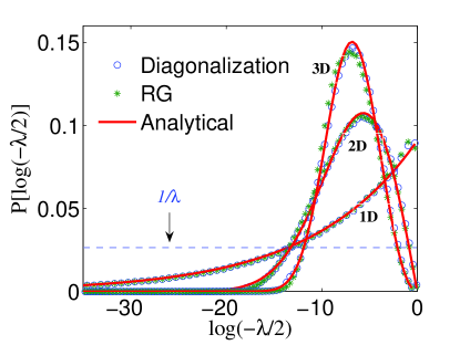
Figure 1: Comparison between the exact numerical diagonalization (circles), and different theoretical approaches: The stars (green) show the results of a renormalization group approach, where, if one considers the problem as finding the normal modes of a spring network, the springs and masses are renormalized. The solid line (red) depicts the analytical results of Eq. (2), and Eq. (11) of the SM. The numerical results shown are for 1, 2 and 3 dimensions, with N=1000, averaged over 1000 realizations. The points were chosen in a line, square or box of side one, and $\epsilon=0.1$, corresponding to $\xi=10^{-4}$ in 1D, $\xi=0.0032$ in 2D and $\xi=0.01$ in 3D. Notice that the graph shows the distribution density of the logarithm of the eigenvalue, which eliminates the governing $1/\lambda$ dependence, and allows us to observe clearly the deviations from it. To demonstrate this, the horizontal dashed line (blue) shows an exact $1/\lambda$ distribution. No fitting parameters are used.

To comprehend the structure of the eigenmodes we use a renormalization group (RG) approach for random systems that was developed in the context of spin chains dasgupta ; fisher ; altman ; gil . At each RG step, we choose the stiffest spring. Since the spring is large by construction, after finding the eigenvalue associated with the stiffest spring we can glue together the two masses at its ends creating a larger mass. At the next RG step we choose again the stiffest spring among those who remain. In this way the large eigenmodes are built initially by pair of masses, but as the RG process progress larger clusters of masses form eigenmodes with smaller eigenvalues. This behavior is demonstrated in Fig. 2.

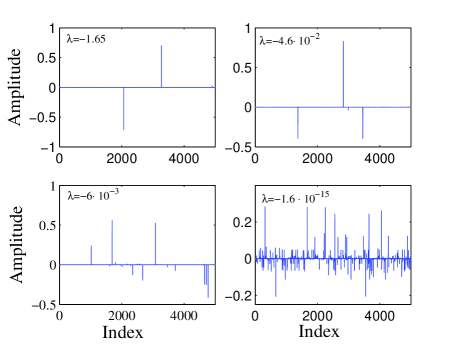
Figure 2: Demonstration of the structure of the eigenmodes. $N=5000$ points were chosen randomly and uniformly in a two dimensional box, with $\epsilon=\xi/r_{nn}=0.1$. The eigenmodes become more delocalized as the eigenvalues approach zero, a condition made quantitative in Eq. (5), through the use of the RG approach. Eigenmodes are comprised of clusters of points, localized in real space.

Since in the RG step a spring is chosen regardless of the masses, the flow of the mass distribution is independent of that of the springs. Namely, we will get statistically the same distribution of clusters as a function of the RG step by a coagulation process where we randomly choose two masses and glue them together at each step. This observation allows us to find the mass distribution as a function of the number of RG steps (see Eqs. (7) and (8) of the SM). Together with the exact result for the eigenvalue distribution, we can find the dependence of the cluster mass on the eigenvalue $n_{c}(\lambda)$, cf Eq. (5).

We will now present in more details the properties of the exponential random matrix model, its applications, and the derivation of $P(\lambda)$ and $n_{c}(\lambda)$

Model and relevant physical problems.- $N$ points are chosen randomly in a $d$ dimensional cube, and $r_{ij}$ is defined as the Euclidean distance between points $i$ and $j$. We define a matrix $A$, as follows: $A_{ij}=e^{-r_{ij}/\xi}$, for $i\neq j$ and $A_{ii}=-\sum_{j\neq i}{A_{ij}}$, the latter definition expressing a conservation law in the physical problem distance_matrices ; amir_glass ; carsten . We shall be interested in determining $P(\lambda)$, the probability density of eigenvalues of the matrix $A$, for low densities (small values of $\epsilon$). Since the matrix is hermitian, it is clear that all its eigenvalues are real, and it can also be proven that they are negative bogomolny2 ; amir_glass .

This model is relevant for problems from various fields of physics, but for now, we choose to focus on scalar phonon localization. It will be useful to have this problem in mind when we discuss the RG calculation.

When studying normal modes of a collection of equal masses $m$ connected by harmonic springs, one has to find the eigenmodes of a matrix $A$, where $\{A_{ij}\}$ are the spring constants, and due to momentum conservation the sum of columns vanishes. The eigenvalues are related to the frequencies by $m\omega^{2}=-\lambda$, where we can choose $m$ to be unity, for convenience. The above model can be used to study phonons in a disordered lattice, where due to the randomness in the matrix elements (i.e., a distribution of spring constants), the oscillating modes may turn out to be localized in space  nagel . Notice that this is a ’scalar’ phonon model schirmacher , where the vectorial properties of the modes have not been taken into consideration (and thus the matrix has $N$ and not $Nd$ modes).

For phonons, the density-of-states of the vibrations $\tilde{P}(\omega)=2m\omega P(\lambda=-m\omega^{2})$ determines the thermal properties of the system Vitelli . It is interesting to note that our result for $P(\lambda)$ implies $P(\omega)\sim 1/\omega$ up to corrections depending on the dimensionality.

Derivation of the eigenvalue distribution.- The exponential matrices model in one dimension has peculiar spectral properties alexander ; ziman . The SM gives a simple, non-rigorous derivation for the low density limit of the eigenvalue distribution in one-dimension, which turns out to be a power-law. The argument also shows that in one dimension the modes are localized, with typical size depending on $\lambda$ as a power-law.

We will now develop a general formula for the eigenvalue spectrum at arbitrary dimension, in the low density limit. We shall see that in one dimension we obtain a power-law, while in higher dimension we get logarithmic corrections to a distribution $P(\lambda)\sim 1/\lambda$ .

Using the following sum:

$$I_{k}\equiv\int P(\lambda)\lambda^{k}d\lambda=\frac{1}{N}\left\langle\sum_{i_{1},i_{2}..i_{k}}A_{i_{1},i_{2}}A_{i_{2},i_{3}}...A_{i_{k},i_{1}}\right\rangle,$$ (1)

one can calculate the $k$’th moment of the probability density. In the SM we find that in the low density approximation $\epsilon\rightarrow 0$, $I_{k}\approx-(-2)^{k-1}d!V_{d}(\epsilon/k)^{d},$ with $V_{d}=\pi^{d/2}/\Gamma(d/2+1)$ the volume of a d dimensional unit sphere.

Since a distribution is fully determined by its moments under certain conditions which are fulfilled in our case moments , it suffices to find a distribution which yields these moments. It can be directly checked by performing the integrals that the following probability density does this:

$$P(\lambda)=\frac{\epsilon^{d}dV_{d}/2[-\rm{log}(-\lambda/2)]^{d-1}e^{-\frac{V_{d}}{2}\epsilon^{d}(-\rm{log}(-\lambda/2))^{d}}}{\lambda}.$$ (2)

The cumulative $C(\lambda)$ of this distribution takes a particularly simple form:

$$C(\lambda)\equiv\int_{\lambda}^{0}P(\lambda)d\lambda=e^{-\frac{V_{d}}{2}\epsilon^{d}(-\rm{log}(-\lambda/2))^{d}}.$$ (3)

In one-dimension we find a power-law divergence in the distribution density, while in a dimension $d>1$ we see from Eq. (2) that there is a finite cutoff at small eigenvalues. Fig. 1 compares this formula with numerical diagonalization, for the one, two and three dimensional cases, as well as the RG procedure.

It is important to distinguish the above result from, for example, those of Ref. [amir_glass, ], which relates the eigenmodes to isolated pairs of points. There, an uncontrolled approximation was used, connecting pairs of nearest-neighbors (a procedure which is not always well-defined). While giving the correct qualitative dependence, it differs from Eq. (2) by a factor of 2 in the exponential, as well as in the normalization factor. As will be shown via the renormalization group approach in the next section, this difference reflects important differences in the underlying physics, and in the structure of the eigenmodes: the high frequency eigenmodes indeed consist of pairs of nearest-neighbors masses, and for them the two approaches coincide. However, the low-lying modes are comprised of an increasing number of masses, diverging as the frequency approaches zero. For any finite value of $\epsilon$, Eq. (2) might be violated for sufficiently small $\lambda$, while keeping the corrections to all moments of the distribution sufficiently small.

Renormalization group approach.- Following dasgupta ; fisher ; altman ; gil , let us consider the renormalization group (RG) approach to this problem. This will enable us to understand the localization properties of the eigenvectors. We recall the scalar phonon localization picture, where the points represent masses and the matrix-elements represent spring constants. At each RG step, we choose the largest spring $K$: due to the broadness of the spring distribution, it will not be affected much by the neighboring springs, and therefore it will contribute a frequency $\omega^{2}=\frac{K}{\mu}=-\lambda$, where $\mu=\frac{m_{1}\cdot m_{2}}{m_{1}+m_{2}}$ is the reduced mass of the two masses it connects, $m_{1}$ and $m_{2}$. Initially, all masses are equal. Notice that the mechanical intuition tells us we should choose the largest spring at each step, and not necessarily the largest frequency, i.e., the choice of the springs does not depend on the masses. Since this spring is large by construction, we can now ’glue’ the two masses together, and create a single mass $m_{1}+m_{2}$. We also have to renormalize the springs attaching the new mass and all other masses: a reasonable way to do so is to take each of the springs between a mass $m$ and the new (joint mass) as the sum of the two springs between the mass $m$ and each of the masses $m_{1}$ and $m_{2}$. Clearly we will obtain smaller frequencies and springs and larger masses as the RG progresses.

As is shown in Fig. (1), this simple scheme captures the essential physics, with no fitting parameters. As mentioned, the reason the method works so well is the broadness of the ’spring’ distribution: for a one dimensional case, for example, the distribution of the nearest-neighbor spring constants (which can be calculated directly from the exponential distribution of the distance intervals) follows a $P(K)\sim 1/K^{1-\epsilon}$, where $\epsilon\rightarrow 0$ in the low density limit. Notice that for the one-dimensional case the RG procedure would choose exactly these nearest-neighbor springs, by construction. Thus, were we to neglect the mass RG we would obtain $P(\lambda)\sim 1/\lambda^{1-\epsilon}$, which recovers the low density result mentioned earlier. In the SM we show how one can incorporate the mass RG to correct the one-dimensional result also for higher densities.

Since at each RG step a spring is chosen regardless of the masses, the flow of the mass distribution is completely independent of that of the springs. As mentioned, the results of the mass RG are applicable for any dimension. We will now show that using the probability density we obtained, Eq. (2), with the results of the mass RG, we can understand the localization properties of the eigenvectors. The SM shows how we can find the distribution of masses at a given stage of the RG process, which turns out to be approximately an exponential distribution $e^{-m/\langle m\rangle}$, with $\langle m\rangle$ changing as the RG process evolves, corresponding to the formation of larger and larger clusters. This implies there is a typical mass $\langle m\rangle$ at each instance. Since at each step of the RG process the number of clusters decreases by one, after $k$ steps the average cluster mass is given by: $\langle m\rangle=N/(N-k)$, which is also the typical size of the cluster, $n_{c}$. On the other hand we can find the relation between the RG step $k$ and the eigenvalue $\lambda$: In the RG process at each step the number of masses is decreased by one, and the corresponding eigenmode recorded, starting with the highest springs (and eigenvalues). At the stage of the RG flow corresponding to an eigenvalue $\lambda$, the number of masses left, $N-k$, can be calculated using Eq. (3):

$$k=N\int_{-2}^{\lambda}P(\lambda)d\lambda=N(1-C(\lambda)).$$ (4)

Combining this equation with that for $n_{c}=\langle m\rangle$, we find that $n_{c}$ depends on the eigenvalue as:

$$n_{c}(\lambda)\sim 1/C(\lambda)=e^{\frac{V_{d}}{2}\epsilon^{d}(-\rm{log}(-\lambda/2))^{d}}.$$ (5)

As we go to zero eigenvalue, the size of the eigenmodes diverges, as demonstrated in Fig. (2) on a particular example. Notice that for the case $d=1$ we recover the power-law relation between localization length and $\lambda$ mentioned earlier, and related to Refs. [alexander, ] and [ziman, ].

Eq. (4) also allows us to count $\mathcal{N}(n_{c})$, the number of all clusters containing more than $n_{c}$ masses: their number is $N\int_{\lambda}^{0}P(\lambda)d\lambda=NC(\lambda)$, where we know the dependence of $\lambda$ on $n_{c}$ through Eq. (5). This gives: $\mathcal{N}(n_{c})/N=1/n_{c}$.

Physical implications.- The mathematical model presented is relevant also for other physical problems besides phonon localization discussed above. For example, one can consider the hopping of a particle in a random environment, where $A_{ij}$ describes the transition probability of a particle from site $i$ to site $j$. If we define the probabilities of the particle to be at the different sites by a vector $\vec{p}$, then $\frac{d\vec{p}}{dt}=A\vec{p}$. In disordered systems, the transition rate often depends exponentially on the distance scher . Another physical example of relevance, is the study of relaxations in glasses. Under certain approximations, this can be mapped to the study of eigenmodes of a class of random matrices related to the one described above amir_glass_related and in fact this has been the original motivation for this study. In both the cases of the diffusion problem and the relaxations in glasses the Laplace transform of the distribution density plays an important role: in the hopping problem, it gives the probability to remain in the origin diffusion_laplace , while for the glass relaxation it corresponds to the time dependence of the relaxation amir_glass ; pollak2 .

Upon taking the Laplace transform $\hat{P}(t)$ of the distribution density in one-dimension (with argument $t$), we obtain $\hat{P}(t)\sim t^{-\frac{\epsilon}{1+\epsilon}}.$ This implies that the diffusion in this case is anomalous scher ; anomalous1 ; anomalous2 : the probability to remain in the origin does not decrease as $1/\sqrt{t}$, as is the case for normal diffusion, but as a smaller power (the particle tends to be more localized). If we assume that after a time $t$ the particle has spread over a distance $r$, it is reasonable to assume that $\hat{p}(t)r\sim 1$, showing that $r\sim t^{\frac{\epsilon}{1+\epsilon}}$. In the case $\epsilon\rightarrow 0$, this can be approximated as $\hat{P}(t)\sim C-\rm{log}(t)$. This type of behavior has been experimentally observed in various types of glassy systems ludwig2 ; Grenet1 ; zvi:3 . In higher dimensions, one obtains in the low density limit $\hat{P}(t)=\phi[\rm{log}(t)]$, with $\phi$ a polynomial of degree $d$. This will be elaborated on in future works.

Summary.- We presented here a model of random matrices which captures the interesting physics of various different systems. After introducing the model, we found the eigenvalue distribution density in the low-density limit (Eq. (2)) and the localization properties of the eigenmodes (Eq. (5)) using a direct moment calculation as well as a renormalization group approach. Our results for the spectrum agree with the 1D case alexander ; ziman , and with the exact numerical diagonalization. While in one dimension it is known that for an infinite system there will be an (integrable) power-law divergence of the spectrum, in a higher dimension $d$ we found that there is a finite cutoff, where $\epsilon=\xi/r_{nn}$ is the small parameter of the theory. We used the RG approach to show that the eigenmodes are localized, and to find a relation between the spatial extent of an eigenmode and the corresponding eigenvalue, implying that this size diverges as the eigenvalue approaches zero.

We discussed the application of the model for various physical problems, such as relaxations in glasses, diffusion of particles in random media, and localization. In the future, it would be fascinating to understand also the crossover or phase-transition to the high density or low disorder regime, which should present different physics.

We thank M. Aizenman, D. Cohen, M. E. Fisher, O. Hirschberg, B. Nedler, W. Schirmacher, V. Vitelli and O. Zeitouni for important discussions. This work was supported by a BMBF DIP grant as well as by ISF and BSF grants and the Center of Excellence Program.

I Supplementary Material

II 1. A nonrigorous derivation in one-dimension

It is known that for an isolated system the center-of-mass motion gives a zero eigenvalue mode, and thus in our model a cluster of points largely separated from the rest of the points will give an exponentially vanishing eigenvalue. Let us consider the statistics for finding such a cluster, isolated on both sides by a distance $r$ (here we explicitly use the one dimensional character of the problem).

By perturbation theory the vanishing eigenvalue will be shifted by a value of order $|\lambda|\sim e^{-r/\xi}$, where $\xi$ was the decay length of the matrix elements. We choose the points from a uniform distribution, hence the distances between them are distributed exponentially. Therefore, if we move (e.g. to the right) along the one dimensional chain, the probability of encountering a gap of size $\tilde{r}$ larger than $r$ is $P(\tilde{r}>r)=e^{-r/r_{nn}}$ with $r_{nn}$ being the average distance between the points. If we proceed to move along the chain we are certain to encounter a gap larger than $r$ eventually. Thus, the probability density of finding a cluster isolated from both sides by a distance $r$ (obtained by differentiating the cumulative distribution) is $p(r)=e^{-r/r_{nn}}/r_{nn}$. Using the relations, $P(\lambda)d\lambda=p(r)dr$ we find $P(\lambda)\propto 1/\lambda^{1-\epsilon}$, with $\epsilon=\xi/r_{nn}$ being a small parameter if the density of points is low enough. This analysis also allows us to find the length of the cluster, since the typical number of points we have to pass until we encounter the second gap is $l(\lambda)=1/p\propto e^{r/r_{nn}}\sim\lambda^{-1/\epsilon}$. This reproduces the low density limit of a similar problem alexander ; ziman , albeit with nearest-neighbor matrix elements only (indeed,in the low density limit, in one dimension, we do not expect next-nearest neighbor couplings to modify the results). The relation $l(\lambda)$ that was obtained implies that the spatial extent of the modes diverges as the eigenvalue approaches zero.

III 2. Calculation of the moments of the eigenvalue probability density

We would like to calculate the $k$’th moment of the probability density using the following sum:

$$\int P(\lambda)\lambda^{k}d\lambda=\frac{1}{N}\langle\sum_{i_{1},i_{2}..i_{k}}A_{i_{1},i_{2}}A_{i_{2},i_{3}}...A_{i_{k},i_{1}}\rangle$$ (6)

To gain intuition, let us consider the first moment: $\int P(\lambda)\lambda d\lambda=\frac{1}{N}\langle\sum_{i}A_{i,i}\rangle.$ By construction, the magnitude of the diagonal elements is the sum of all the other elements in the columns, i.e., sum of the hopping matrix elements to all neighbors, close and far. To the lowest order in $\epsilon$, we can consider only the nearest-neighbor of each point, as we shall shortly demonstrate. Under this approximation the first moment can be readily calculated: $I_{1}\equiv\int P(\lambda)\lambda d\lambda\approx-\int_{0}^{\infty}P_{nn}(r)e^{-r/\xi}dr,$where $P_{nn}(r)$ is the nearest-neighbor distance distribution, which is given by $P_{nn}(r)=\frac{dV_{d}}{r_{nn}}{(r/r_{nn})}^{d-1}e^{-V_{d}{(r/r_{nn})}^{d}}$, where $V_{d}$ is the volume of a $d$ dimensional sphere and $r_{nn}$ is the average nearest-neighbor distance. In the low density limit this gives $I_{1}\approx-d!V_{d}\epsilon^{d}.$ Calculating the corrections to this formula due to all neighbors, one obtains a correction of the order of $O(\epsilon^{2d})$, which is indeed of higher order in the small parameter $\epsilon$. The crux of the matter here is that due to the exponential function, the contributions to the integral arise mainly from rare pairs which are very close to each other, with a distance of order $\xi$ between them. For such pairs the probability that a third point will be in the vicinity of the two points is negligible.

For the $k$’th moment the general term contributing will be a combination of hops to the nearest-neighbor and loops that stay in either the original site or the nearest-neighbor, as illustrated schematically in Fig. 3. Thus, there would be $2^{k-1}$ contributing diagrams, each of equal contribution. Therefore the $k$’th moment will be given by $I_{k}\equiv\int P(\lambda)\lambda^{k}d\lambda\approx-(-2)^{k-1}\int_{0}^{\infty}P_{nn}(r)e^{-kr/\xi}dr.$ This yields in the low density limit: $I_{k}\approx-(-2)^{k-1}d!V_{d}(\epsilon/k)^{d}.$ These moments correspond to the probability density given in Eq. (2), as can be verified by a direct calculation of its moments.

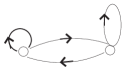
Figure 3: An example of a diagram contributing to the $k$’th moment in the low density limit.

It is interesting to note that although the leading order contribution to the k’th moment was made by a small subset of configurations, close pairs, the resulting distribution captures the probability density of eigenvalues whose corresponding eigenmodes are actually clusters. The clusters can understood by the renormalization group approach, discussed in the manuscript. It is generally true that for large k’s, the moments are dominated by the largest (i.e., most negative) eigenvalues, which in our case are exactly the close pairs (which are nearly eigenmodes). The above calculation shows that in the low density limit also the low moments (e.g: $I_{1}$, above), are dominated by the close pairs. Thus, we can find all moments and the complete distribution, by studying the properties of the close pairs, in a similar fashion to an analytical continuation, by which studying the function in a small region determines its behavior further away.

In the case of matrix elements decaying not exponentially but as some function $f(r)$ of the distance, we can repeat the previous argumentation. If $f(r)$ decays, for example, faster than exponential, than surely the contribution of the diagrams neglected will be smaller still, thus justifying the method. In this case the k’th moment will be: $I_{k}\equiv\int P(\lambda)\lambda^{k}d\lambda\approx-(-2)^{k-1}\int_{0}^{\infty}P_{nn}(r)f(r)^{k}dr.$ It can be checked that the cumulative of the associated distribution in this case is given by:

$$C(\lambda)\equiv\int_{\lambda}^{0}P(\lambda)d\lambda=e^{-\frac{V_{d}}{2r_{nn}^{d}}((f^{-1}(-\lambda/2))^{d}},$$ (7)

where $f^{-1}$ is the inverse function of $f(r)$. As an example, applying this formula for gaussian matrix elements in two-dimensions gives a power-law distribution density, $P(\lambda)\sim 1/\lambda^{1-\pi\epsilon^{2}/2}$.

IV 3. Solution for the renormalization of the masses

As explained in the manuscript, the RG procedure chooses the largest springs at every instance. With regard to the masses this is a random process not depending explicitly on the masses, as long as we neglect effects arising from the larger surface area of the clusters. As is shown in the manuscript, these do not affect $\langle m\rangle$. We shall now analyze the resulting flow of the mass distribution, under this approximation. Initially, we have a set of unit masses, and at each step we choose two masses at random and combine them. If we denote the average number of masses of mass m in the k’th stage as $N^{k}_{m}$ (at which step we have $N-k$ masses left), we therefore have:

$$N^{k+1}_{m}\approx N^{k}_{m}-\frac{2N^{k}_{m}}{N-k}+\sum_{m^{\prime}=1..(m-1)}\frac{N^{k}_{m^{\prime}}}{N-k}\frac{N^{k}_{m-m^{\prime}}}{N-k}$$ (8)

Indeed, the probability that a chosen mass is of mass $m$, is $\frac{N^{k}_{m}}{N-k}$. This relates to the first term, which accounts for the average reduction in the number of masses of mass $m$ (the factor of two arising from the fact that we choose two masses at each stage). The second term accounts for all the possible ways that two smaller masses can combine to contribute to the number of masses of mass $m$, where again the same form for the probabilities enters.

In order to move from numbers to probabilities, we have to divide by the current number of masses, which is $N-k-1$ (since at each RG step, when two masses are combined to create one mass, we lose one mass). It is useful to write, for $N-k\gg 1$:

$$\frac{1}{N-k-1}\approx\frac{1}{N-k}+\frac{1}{(N-k)^{2}}.$$ (9)

Denoting by $\mathcal{P}^{k}_{m}$ the probability to have a mass of size $m$ after $k$ springs are eliminated, we have $P^{k}_{m}=\frac{N^{k}_{m}}{N-k}$, leading to:

$$P^{k+1}_{m}\approx P^{k}_{m}+\frac{P^{k}_{m}}{N-k}-\frac{2P^{k}_{m}}{N-k}+\frac{1}{N-k}\sum_{m^{\prime}=1..(m-1)}P^{k}_{m^{\prime}}P^{k}_{m-m^{\prime}}.$$ (10)

Thus, we finally obtain:

$$\Delta P_{m}\approx-\frac{P_{m}}{N-k}+\frac{1}{N-k}\sum_{m^{\prime}=1..(m-1)}P_{m^{\prime}}P_{m-m^{\prime}},$$ (11)

where the second term of Eq. (9) changed the factor of two appearing in Eq. (8) to be one.

It is now straightforward to take the continuous limit, where it is convenient to define a fictitious time related to the step number as $t=-\log\frac{N-k}{N}$. This leads to the following integro-differential equation for the time evolution of the masses:

$$\frac{\partial\mathcal{P}(m,t)}{\partial t}=-\mathcal{P}(m,t)+\int_{0}^{m}\mathcal{P}(m^{\prime},t)\mathcal{P}(m-m^{\prime},t)dm^{\prime},$$ (12)

where the time $t$ is related to step number $k$ by the equation $t=-\rm{log}[(N-k)/N]$. This is a particular case of the Smoluchowski coagulation equation smoluchowski . It can be verified that:

$$\mathcal{P}(m,t)=e^{-e^{-t}m}e^{-t},$$ (13)

is a solution. We expect this solution to be relevant for $t\gg 1$, when the slightly different initial conditions it obeys are not important aizenman_bak (initially, all masses are equal, not exponentially distributed).

V 4. RG solution in one dimension

In the following we show how in one dimension one can find $P(\lambda)$ with the RG approach, without using the result of the moment calculation. Eq. (13) shows that the mass distribution at a given time is given by $\mathcal{P}(m,t)=e^{-e^{-t}m}e^{-t}$. From this, we can calculate $\langle 1/m\rangle=\int\frac{\mathcal{P}(m,t)}{m}dm$. Approximating the exponential as an effective cutoff at $m_{c}=e^{t}$, we find that $\langle 1/m\rangle\sim\rm{log}(m_{c})e^{-t}\sim te^{-t},$ where we took a lower cutoff of order unity for the mass.

Using the relation between $t$ and $k$ we find that:

$$\langle 1/m\rangle\sim(N-k)/N,$$ (14)

where $N-k$ is the number of masses left after $k$ RG steps.

For the one dimensional case we can combine this result with the previously obtained renormalization of the springs, to obtain the mass correction. Since the eigenmodes obey $\omega^{2}=K/\mu$, with $\mu$ the reduced mass of the two current masses, the springs eliminated at this point of the RG flow, whose distribution was shown to obey $P(K)\sim 1/K^{1-\epsilon}$, contribute on average to

$$-\lambda=\omega^{2}=K\langle 1/m_{1}+1/m_{2}\rangle=2K\langle 1/m\rangle=2K^{1+\epsilon}.$$ (15)

Calculating the distribution of $\lambda$ arising from the known spring distribution $P(K)$ gives

$$P(\lambda)\sim 1/\lambda^{\frac{1}{1+\epsilon}},$$ (16)

where the lower cutoff is still $\lambda=0$ but the higher cutoff is $\lambda=-2$. Thus, the effect of the mass RG in one dimension is changing $P(\lambda)\sim 1/\lambda^{1-\epsilon}$ to $1/\lambda^{\frac{1}{1+\epsilon}}$, which is negligible for small $\epsilon$. For low densities the RG approach and the derivation via the calculation of the moments give identical results, as they should.

References

- (1) M. Mehta, Random Matrices (Academic Press, New York, 1991).
- (2) I. M. Lifshitz, Adv. Phys. 13, 482 (1964).
- (3) C. Dasgupta and S.-K. Ma, Phys. Rev. B 22, 1305 (1980).
- (4) D. S. Fisher, Phys. Rev. B. 50, 3799 (1994); D. S. Fisher, Phys. Rev. B. 51, 6411 (1995).
- (5) E. Altman, Y. Kafri, A. Polkovnikov, and G. Refael, Phys. Rev. Lett. 93, 150402 (2004).
- (6) T. E. Lee et al., Phys. Rev. E 80, 046210 (2009).
- (7) M. Mezard, G. Parisi, and A. Zee, Nuclear Physics B 3, 689 (1999).
- (8) A. Amir, Y. Oreg, and Y. Imry, Phys. Rev. B 77, 165207 (2008).
- (9) C. Timm, Phys. Rev. E. 80, 021140 (2009).
- (10) E. Bogomolny, O. Bohigas, and C. Schmit, arXiv:0710.2063 (2008).
- (11) S. R. Nagel, A. Rahman, and G. S. Grest, Phys. Rev. Lett 47, 1665 (1981).
- (12) W. Schirmacher and M. Wagener, Phil. Mag. B 65 4, 607 (1992).
- (13) V. Vitelli et al., Phys. Rev. E 81, 021301 (2010).
- (14) S. Alexander, J. Bernasconi, W. R. Schneider, and R. Orbach, Rev. Mod. Phys. 53, 175 (1981).
- (15) T. A. L. Ziman, Phys. Rev. Lett 49, 337 (1982).
- (16) It is sufficient that the moments grow slowly enough such that the power series they generate has a finite radius of convergence, see W. Feller, Introduction to the Theory of Probability and Its Applications, Wiley, New York (1971), vol. 2, p. 514 .
- (17) H. Scher and M. Lax, Phys. Rev. B. 7, 4502 (1973); H. Scher and E. W. Montroll, Phys. Rev. B 12, 2455 (1975); H. Scher, private communication (2009).
- (18) A. Amir, Y. Oreg, and Y. Imry, Phys. Rev. B 77, 165207 (2008); A. Amir, Y. Oreg, and Y. Imry, Phys. Rev. Lett. 103, 126403 (2009); A. Amir, Y. Oreg, and Y. Imry, Ann. Phys. (Berlin) 18,12, 836 (2009).
- (19) To see this, one can write the probability to remain in a given site in terms of the eigenmodes and eigenvalues, as: , with the corresponding eigenmodes. Averaging over gives , which, in the continuous limit, is the Laplace transform of the probability density.
- (20) M. Pollak and Z. Ovadyahu, Phys. Stat. Sol. (c) 2, 283 (2006).
- (21) J.-P. Bouchaud and A. Georges, Physics Reports 195, 127 (1990).
- (22) R. Metzler and J. Klafter, J. Phys. A 37, R161 (2004).
- (23) S. Ludwig and D. Osheroff, Phys. Rev. Lett. 91, 105501 (2003).
- (24) T. Grenet, Eur. Phys. J. B 32, 275 (2003).
- (25) A. Vaknin, Z. Ovadyahu, and M. Pollak, Phys. Rev. Lett. 84, 3402 (2000).
- (26) M. von Smoluchowski, Phys. Z. 17, 557 (1916).
- (27) M. Aizenman and T. Bak, Commun. Math. Phys. 65, 203 (1979).