The JCMT Legacy Survey of the Gould Belt: a first look at Taurus with HARP

Abstract

As part of a JCMT Legacy Survey of star formation in the Gould Belt, we present early science results for Taurus. CO J=3-2 maps have been secured along the north-west ridge and bowl, collectively known as L 1495, along with deep ¹³CO and C¹⁸O J=3-2 maps in two sub-regions. With these data we search for molecular outflows, and use the distribution of flows, HH objects and shocked H₂ line emission features, together with the population of young stars, protostellar cores and starless condensations to map star formation across this extensive region. In total 21 outflows are identified. It is clear that the bowl is more evolved than the ridge, harbouring a greater population of T Tauri stars and a more diffuse, more turbulent ambient medium. By comparison, the ridge contains a much younger, less widely distributed population of protostars which, in turn, is associated with a greater number of molecular outflows. We estimate the ratio of the numbers of prestellar to protostellar cores in L 1495 to be $\sim$1.3–2.3, and of gravitationally unbound starless cores to (gravitationally bound) prestellar cores to be $\sim$1. If we take previous estimates of the protostellar lifetime of $\sim$5$\times$10⁵ yrs, this indicates a prestellar lifetime of 9($\pm$3)$\times$10⁵ yrs. From the number of outflows we also crudely estimate the star formation efficiency in L 1495, finding it to be compatible with a canonical value of 10-15%. We note that molecular outflow-driving sources have redder near-IR colours than their HH jet-driving counterparts. We also find that the smaller, denser cores are associated with the more massive outflows, as one might expect if mass build-up in the flow increases with the collapse and contraction of the protostellar envelope.

1 Introduction

The Gould Belt Survey (GBS: Ward-Thompson et al., 2007a) is a large, legacy programme currently underway at the James Clerk Maxwell Telescope (JCMT). The goal is to gather both heterodyne line observations and submillimetre (submm) continuum images of nearby star forming regions. The survey targets the Gould Belt, which is a ring of O-type stars and molecular clouds with a radius of $\sim$350 pc. It is inclined at $\sim$20^∘ to the Galactic Plane and is centred on a point 200 pc from the Sun (ascending node, $\Omega=275-295$; Torra, Fernández & Figueras, 2000). The Gould Belt includes well known regions such as Orion, Taurus-Auriga-Perseus, Serpens, Lupus, Ophiuchus and the Pipe nebula. Taurus is one of four regions initially targeted in ¹²CO J=3-2 (hereafter CO 3-2), ¹³CO 3-2, and C¹⁸O 3-2. These four regions – Orion A (Buckle et al., 2010), Serpens (Graves et al., 2010), Ophiuchus (White et al., in prep.) and Taurus (this paper) – were selected as being complementary, active, nearby, relatively well known, and well studied. Extensive submm continuum mapping, at 450 $\mu$m and 850 $\mu$m, is also planned as part of the survey (Ward-Thompson et al., 2007a).

In studies of nearby, low-mass star forming regions CO 3-2 emission samples the denser, warmer gas which often envelopes cores where new stars are forming (temperatures $\sim 10-50$ K; gas densities of the order of $10^{4}-10^{5}$ cm^-3). CO 3-2 is also a proven tracer of outflow activity (e.g. Hatchell, Fuller & Ladd 1999; Knee & Sandell 2000; Davis et al. 2000a; Hatchell, Fuller & Richer 2007a; Lee et al. 2007; Bussmann et al. 2007; Yeh et al. 2008). With the JCMT, moderate spatial resolution is attainable at 345 GHz ($\sim$14″), which often allows one to disentangle multiple outflows in clustered regions. The higher critical density for excitation of the 3-2 line (over, say, the 1-0 emission line) can also lead to better maps of the dense, more collimated flow components. Molecular outflows are known to emanate from the very youngest sources, objects that are still accreting most of their final mass. New, large-scale surveys in CO can therefore be used to identify the locations of these embedded protostars, leading to a more complete census of the youngest stars, and an indication of the overall youth and star formation activity in a region (e.g. Hatchell et al., 2007a; Davis et al., 2008; Hatchell & Dunham, 2009; Buckle et al., 2010).

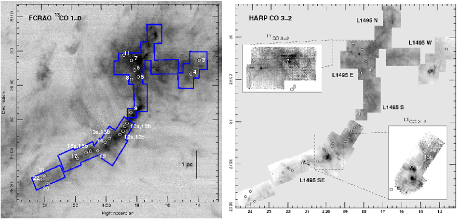
Figure 1: Left - an overview of L 1495 in the north-west corner of Taurus. The image shows integrated ¹³CO 1-0 emission from the FCRAO survey of Goldsmith et al. (2008). The positions of the H¹³CO⁺ cores identified by Onishi et al. (2002) are marked with circles and labelled using their core numbering scheme. Right - a complete map of all regions observed with HARP in CO 3-2 (intensity integrated between 2.0 and 11.0  km s^-1), with the positions of the H¹³CO⁺ cores again marked. The areas mapped in ¹³CO and C¹⁸O 3-2 are also indicated; maps of ¹³CO emission, integrated between 4.9 and 9.1  km s^-1(L 1495 E) and 4.5 and 8.2  km s^-1(L 1495 SE), are shown inset as grey-scale images. In the main text we refer to L 1495 N, E, S and W as the bowl, and L 1495 SE as the south-east ridge.

Table 1: Log of CO 3-2 observations in L 1495.

Regiona	Areaa	Cubea	Datea	RAb	Decb	PAc	Map sizec	$v_{o}$d
				(J2000.0)	(J2000.0)			( km s-1)
Bowl	L 1495 E	L 1495	2007-11-24	4:18:04.8	28:21:45	90∘	20′$\times$10′	6.6-7.1
′′	′′	L 1495-S	2007-12-22	4:17:50.0	28:09:00	0∘	10′$\times$15′	5.9-6.7
′′	′′	L 1495-S2	2008-09-17	4:18:48.0	28:14:30	0∘	10′$\times$10′	$\sim$5.9-6.7
′′	L 1495 N	L 1495-NE1	2008-11-08	4:16:59.0	28:30:13	0∘	10′$\times$14′	$\sim$6.7
′′	′′	L 1495-NE2	2009-01-30	4:16:28.1	28:45:33	0∘	10′$\times$14′	$\sim$6.7
′′	L 1495 S	L 1495-S3	2008-11-08	4:17:34.0	27:49:20	0∘	10′$\times$22′	6.6-6.8
′′	′′	L 1495-SE1	2008-03-29	4:18:09.1	27:35:17	0∘	5′$\times$5′	5.6
′′	L 1495 W	L 1495-W	2008-08-21	4:14:10.0	28:12:00	0∘	10′$\times$10′	6.7
′′	′′	L 1495-W1	2009-01-31	4:15:54.7	28:16:33	0∘	22′$\times$10′	$\sim$6.7
′′	′′	L 1495-W2	2008-10-07	4:14:34.0	28:04:00	0∘	13′$\times$13′	6.7
′′	′′	L 1495-W3	2009-01-30	4:13:35.0	28:22:13	0∘	13′$\times$13′	6.7
Ridge	L 1495 SE	L 1495-SE2	2008-03-15	4:18:41.3	27:22:00	147∘	8′$\times$15′	5.3-5.7
′′	′′	L 1495-SE3	2007-11-25	4:19:42.4	27:13:24	147∘	8′$\times$15′	6.5
′′	′′	L 1495-SE3b	2008-01-12	4:20:10.0	27:05:00	147∘	10′$\times$10′	6.4
′′	′′	L 1495-SE3c	2008-09-17	4:19:22.0	27:04:06	147∘	9′$\times$23′	$\sim$6.4
′′	′′	L 1495-SE4	2008-08-21	4:21:14.1	27:01:11	113∘	10′$\times$20′	6.6-6.7
′′	′′	L 1495-SE4b	2008-10-07	4:22:22.0	26:55:00	113∘	10′$\times$10′	$\sim$6.6
′′	′′	L 1495-SE5	2008-11-08	4:23:44.5	26:39:00	113∘	9′$\times$ 25′	6.6-6.7

^aThe areas in the bowl and ridge regions of L 1495 are made up of multiple data cubes, often observed on different nights.

^bCoordinates of the cube centres.

^cCube map size and position angle of the map long axis (measured E of N); with “basket-weave” mapping the scan direction is along

and orthogonal to this axis.

^dThe LSR velocities of the H¹³CO⁺ cores found in or near (if an approximate value is given) each region by OMK02, which we adopt as the local ambient gas velocity.

Taurus is a much-studied region of low mass star formation (see Kenyon, Gómez & Whitney 2009, for a detailed review). The Taurus molecular cloud covers an area in excess of 100 deg² (Ungerechts & Thaddeus, 1987; Narayanan et al., 2008; Goldsmith et al., 2008). LDN 1495 (L 1495 hereafter) is one of three main areas associated with a high density of young stars. L 1495 lies in the north-west corner of Taurus and coincides with Barnard dark nebulae B 7, 10, 209, 211, 213 and 216. In molecular line and extinction maps L 1495 comprises an extended, knotty filament – here referred to as the “south-east ridge” – and, at its northern extremity, a more diffuse cloud – the “bowl”. Goldsmith et al. (2008) refer to the ridge as B 231 and label only the bowl L 1495. From their extensive CO observations they estimate masses of 1095  M_⊙ and 2626  M_⊙ for the ridge and bowl, respectively, and assign areas of 13.7 pc² (2.3 sqr degrees) and 31.7 pc² (5.3 sqr. degrees) for each region (see their Table 4). They also note that, quite remarkably, the SE ridge is 75′ (3 pc) long yet only 4.5′ (0.2 pc) wide. A similar collimated feature in the NGC 6334 star forming region has recently been analysed by Matthews et al. (2008).

In this paper we split the bowl into four areas, L 1495 N, S, E and W, and label the ridge L 1495 SE. L 1495 E harbours the classical T Tauri star (TTS) CoKu Tau-1 and HH 156 (Eislöffel & Mundt, 1998); L 1495 W (B 209) is associated with the TTS CW Tau (Elias 1, Hubble 4) which drives HH 220 and possibly also HH 826-828 (Gómez de Castro, 1993; McGroarty & Ray, 2004). HH 390/391/392 and HH 157 are located along the L 1495 SE ridge (Gomez, Whitney & Kenyon 1997; Eislöffel & Mundt 1998); HH 157 is driven by the TTS Haro 6-5B (FS Tau B) and comprises a spectacular HH jet and bow shock that extend over 30″–40″.

L 1495 W has been mapped in C¹⁷O 1-0, C¹⁸O 1-0, CS 2-1, N₂H⁺ 1-0 (at FCRAO) and in NH₃ (1,1) and (2,2) emission (at Effelsberg) by Tafalla et al. (2002) – the region they label “L 1495” roughly coincides with L 1495 W. N₂H⁺ 1-0 maps of the south-east ridge are presented by Tatematsu et al. (2004). More extensive ¹³CO and C¹⁸O 1-0 maps of Taurus are discussed by Mizuno et al. (1995), and Onishi et al. (1996); CO and ¹³CO 1-0 maps, covering 98 square degrees with 45″ resolution, have recently been published by Narayanan et al. (2008) and Goldsmith et al. (2008). Finally, extensive yet high spatial resolution H¹³CO⁺ 1-0 observations of the molecular cores in Taurus, including the L 1495 ridge and bowl, are discussed by Onishi et al. (2002, hereafter referred to as OMK02). These H¹³CO⁺ observations, to which we refer throughout the paper, were obtained at the 45 m Nobeyama telescope with a beam width of 20″.

Kenyon & Hartmann (1995) present a list of $\sim$300 Young Stellar Objects (YSOs) in Taurus, derived from multi-wavelength observations and complemented recently with data from the Spitzer Space Telescope (Hartmann et al., 2005; Luhman et al., 2006, though note that the Spitzer observations do not cover L 1495 W or the bottom of the south-east ridge). Many of the youngest sources have been observed in the 1.3 mm continuum survey obtained by Motte & André (2001). In L 1495 the young stars are clustered toward the eastern and western sides of the L 1495 bowl, and are tightly bound along the narrow, south-east ridge. The protostellar population as a whole is discussed in the review of Kenyon et al. (2009), who also present an updated list of YSOs in Taurus. Kenyon et al. note in their article that classical TTSs typically have near-infrared (near-IR) colours $H-K_{s}<1-1.5$ and mid-infrared (mid-IR) colours [3.6]-[4.5]$\sim$0.5-1.0 and [5.8]-[8.0]$\sim$0.25-0.75; embedded protostars (Class 0/I sources) are expected to be redder.

In this paper we use an up-to-date list of “Taurus Young Stars”, kindly provided by K. Luhmann, to search for candidate outflow sources in L 1495. This list is essentially the same as that presented by Kenyon et al. (2009). We also assume that “starless” cores are low mass ($M<10$  M_⊙) dense cores without compact luminous sources of any mass (Di Francesco et al., 2007). “Prestellar” cores are a subset of starless cores, since they must also be gravitationally bound (Ward-Thompson et al., 2007b). Establishing whether a core is bound or not is observationally very difficult (although the virial theorem gives some indication). We therefore refer to cores that are not obviously associated with a young star as starless; cores that do appear to contain a young star are referred to as “protostellar”.

Traditionally, a distance of 140 pc has been used for Taurus (Ungerechts & Thaddeus, 1987; Elias, 1978), on the basis of estimates from star counts (McCuskey, 1939), the reddening of field stars as a function of distance (Gottlieb & Upson, 1969), and photometric distances measured to the exciting stars of reflection nebulae (Racine, 1968). Analysis of the velocity field in wide-field molecular line studies suggests that ambient gas velocities change by only a few  km s^-1 across Taurus, and are particularly limited across L 1495 (Ungerechts & Thaddeus, 1987; Narayanan et al., 2008; Goldsmith et al., 2008, see also Sect. 3.1 below). This supports a more-or-less common distance to the molecular clouds and star forming regions in Taurus. Recent trigonometric parallax measurements suggest that the eastern portion of Taurus may be furthest from us, at a distance of $\sim 161$ pc, with the south (around T Tau) at an intermediate distance of 147 pc and the west, L 1495, marking the near side of the cloud at a distance of 130 pc (Torres et al., 2009). However, these distances are based on parallax measurements for only a handful of stars. We therefore adopt the canonical distance of 140 pc for L 1495, consistent with previous studies, most notably Goldsmith et al. (2008) and OMK02.

Overall, our goal with this paper is to search for outflows in L 1495, identify their driving sources, and compare the properties of these outflows with those of the driving sources and associated molecular cores.

2 Observations and Data Reduction

2.1 Data Acquisition

As part of the JCMT Gould Belt Legacy Survey, the 325–375 GHz heterodyne receiver array HARP was used to map 18 near-contiguous regions across the L 1495 bowl and along the south-east ridge in CO 3-2 emission (Fig. 1 and Table LABEL:obs), as well as two smaller sub-regions in ¹³CO 3-2 and C¹⁸O 3-2 emission. HARP is a 16 receptor (4$\times$4 array) single side-band SIS receiver system acting as a front-end to the ACSIS digital auto-correlation spectrometer (Hovey et al., 2000; Smith et al., 2003; Buckle et al., 2009).

CO 3-2 data at a rest frequency of 345.79599 GHz were acquired in dual sub-band mode. Maps with modest and high spectral resolution were acquired simultaneously, with 1024 ACSIS channels covering a bandwidth of 1.0 GHz at a spectral resolution of 977 kHz (0.85 kms^-1), and with 4096 channels covering a bandwidth of 250 MHz at a spectral resolution of 61 kHz (0.05 kms^-1). Only the latter are presented in this paper. In separate observations, ¹³CO 3-2 (330.58796 GHz) and C¹⁸O 3-2 (329.33055 GHz) data were acquired simultaneously in dual sub-band mode using only the high spectral resolution set-up. At these frequencies the telescope Half Power Beam Width measures 14″, corresponding to 0.0095 pc at a distance of 140 pc.

Maps were obtained by scanning the telescope along rows parallel to the sides of the pre-defined mapping areas, each row separated by half or a quarter of an array to improve the spatial sampling. This map is then repeated but by scanning in a perpendicular direction. This strategy of “basket weaving” helps to generate flatter maps and evens out the noise in the final data cube. For most of the data presented here, 2–4 receptors were inoperable; for those fields where 4 receptors were unavailable (regions S2, W2, SE3c and SE4b) the array was stepped by a quarter of the array to prevent empty spaces or poorly sampled regions in the final maps.

Depending on map size, the ¹²CO data cubes were obtained by integrating for 0.6 sec or 1.2 sec (the “sample time”) for each 7.3″ pixel on the sky. A reference position (usually observed at the end of each row in a scan), located at $4^{h}12^{m}24.9^{s}$ (J2000.0) 26^∘50′ 39″, was used throughout. A sample time of 1.0 sec was used with the smaller ¹³CO/C¹⁸O maps.

The CO 3-2 data were observed in grade 3 weather ($\tau$(225 GHz) $\sim$ 0.08–0.12); better weather ($\tau$(225 GHz) $\sim$ 0.05–0.065) was used for the ¹³CO 3-2 and C¹⁸O 3-2 data. System temperatures for the ¹²CO data ranged from 340 to 580 K ($<$450 K in most regions); for the isotopologues temperatures were typically 300-500 K.

The regions mapped in ¹²CO are listed in Table LABEL:obs; these were defined based on large-scale extinction maps (Dobashi et al., 2005), the surveys of dense cores conducted by OMK02, and the locations of Herbig-Haro (HH) objects. Only regions with bright ¹²CO emission were mapped in ¹³CO and C¹⁸O: two overlapping maps centred near H¹³CO⁺ cores 6, 7 and 11 were repeated a number of times to reduce the noise in the final cube; the full map covers an area of $\sim$22′$\times$12′, although note that the noise is roughly a factor of two higher in the north and west portion ($\sim$60%) of the map. Similarly, two overlapping maps covering cores 13a, 13b and 14 were repeated in the L 1495 SE ridge; in this case, the map covers a rectangular area of approximately 20′$\times$6′, though again the north-west quarter of the map is about 3-times noisier than the rest of the data cube. In all, eleven overlapping maps were co-added in L 1495 E, and eleven in L 1495 SE. The regions covered in ¹³CO and C¹⁸O are marked in Fig. 1.

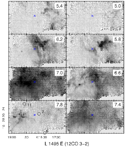
Figure 2: ¹³CO 3-2 channel maps across L 1495 E, plotted between 4.8 and 8.0  km s^-1, in 0.4  km s^-1 intervals. H¹³CO⁺ cores are marked and labelled bottom-left; the small cross in the centre of each map is drawn as a reference marker. The velocity of the channel is marked top-right in each panel.

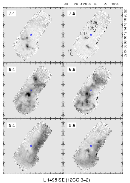
Figure 3: ¹³CO 3-2 channel maps across L 1495 SE, plotted between 5.15 and 8.15  km s^-1, in 0.5  km s^-1 intervals. H¹³CO⁺ cores are marked and labelled top-right; the small cross in the centre of each map is drawn as a reference marker.The velocity of the channel is marked top-left in each panel.

2.2 Data processing

The individual CO 3-2 data cubes listed in Table LABEL:obs (third column) were reduced using the automated ORAC-DR pipeline (Cavanagh et al., 2008). Bad or overly noisy spectra were identified by the pipeline, based on quality assurance criteria stipulated for the Gould Belt Survey legacy data, and these were first removed and noisy regions at the band edges trimmed. The resulting time-series data were re-gridded to a 3D data cube and regions of line emission identified and masked out. A fifth-order polynomial was fit to the resulting emission-free regions and subtracted from each reduced cube. Cubes observed at the same spatial and spectral position were combined and a new baseline region mask was determined from this higher signal-to-noise cube. This was applied to the individual cubes, which were then mosaicked and co-added together using a light Gaussian smoothing kernel with a Full Width Half Maximum (FWHM) $\sim$7.3″, to produce the final cubes and images. The inverse of this baseline mask identifies the line emission regions and this was used to determine the integrated intensity and velocity images presented in this paper. Note that the Gaussian smoothing results in a spatial resolution to point sources of about 16″.

Special care was taken to remove striping from the data cubes when present (Curtis et al., 2010). This was done by determining the receptor-to-receptor response for the whole time-series, and dividing that response out. This technique does assume a priori that each receptor is exposed to similar emission during the scan. Given the diffuse and extended nature of the CO emission from Taurus, this technique worked well in eliminating or, at the very least, in minimising the striping.

In CO 3-2 the noise is relatively uniform across the extensive region mapped. In the un-binned data (at the full 0.05 km s^-1 resolution), at velocities within a few  km s^-1 of the ambient, the root-mean-square (RMS) noise level ($T_{A}^{*}(rms)$) measures 0.10–0.20 K in L 1495-E, N and S (being highest in the south), 0.08–0.15 K in L 1495-W (highest in the north-west), and 0.08–0.16 K along the south-east ridge (it is a little higher, $\sim$0.22 K, in the data around cores 10, 10b and 12a).

The ¹³CO and C¹⁸O data were reduced in the same way. As noted above, the maps in ¹³CO and C¹⁸O were repeated a number of times. We found that in order to produce the optimal coadded map, the worst quality data had to be discarded before being included in the map reconstruction. This was done by measuring the RMS of each of the spectra in the input data and masking those with the highest RMS before generating the map. An iterative method was used to determine the optimal RMS value to apply as a mask. In each step of the iteration, the data were masked using a different limiting RMS before being reconstructed into a map using the Starlink MAKECUBE routine (Jenness et al., 2008). The RMS in the reconstructed map was then measured. The limiting RMS was varied to produce a reconstructed map with the lowest RMS. This map was taken to be the optimal map. In the final, coadded maps the RMS noise level measures $T_{A}^{*}(rms)\sim$0.13-0.20 K in ¹³CO and $\sim$0.16-0.25 K in C¹⁸O at the unbinned spectral resolution of 0.05  km s^-1. As mentioned earlier, the noise level is somewhat higher in the north-west regions of each map.

In this article all images are presented in units of antenna temperature ($T^{*}_{A}$). When calculating outflow parameters, integrated antenna temperature has been converted to main beam brightness temperature, $T_{b}=T^{*}_{A}/(\eta_{mb})$, using an aperture efficiency $\eta_{mb}=0.63$ (Buckle et al., 2009).

3 Results

3.1 Overall distribution of CO 3-2 emission and large-scale velocity structure

The entire region mapped in CO 3-2 with HARP is shown in Fig. 1, where we also show integrated ¹³CO 3-2 images of the L 1495-E and L 1495 SE regions observed in this isotopologue (and in C¹⁸O – data not shown). For comparison purposes, we also present the ¹³CO 1-0 map of Goldsmith et al. (2008).

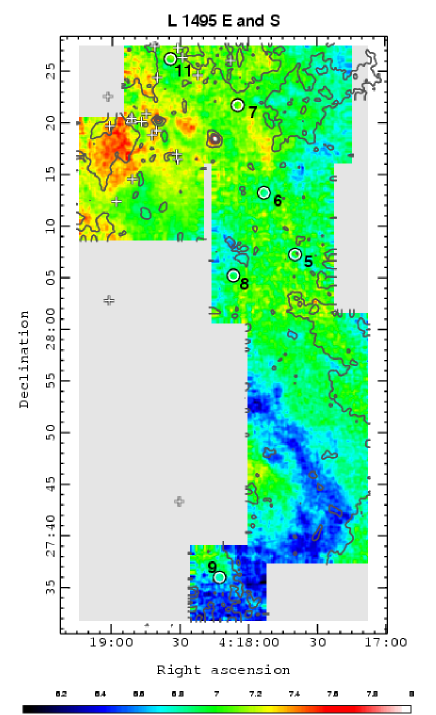
Figure 4: A plot of intensity-weighted radial velocity (first moment) showing the distribution of blue and red-shifted CO 3-2 emission around L 1495 E and L 1495 S. Black/blue through to red/white display velocities in the range 6.0 to 8.0  km s^-1 (green/yellow represent intermediate velocities). Circles, crosses and triangles mark the positions of H¹³CO⁺ cores (labelled), YSOs and HH objects, respectively. Integrated CO 3-2 emission (zeroth moment, from Fig. 1) is over-plotted as contours; levels measure 4,6,8,10,12 K  km s^-1. Note that there is CO 3-2 line emission throughout this entire map.

When mapping L 1495 in CO 3-2 we followed the high-extinction ridge of dense cores observed in C¹⁸O 1-0 and H¹³CO⁺ 1-0 by Onishi et al. (1996) and OMK02, respectively; the ridge is evident in the ¹³CO 1-0 integrated intensity map reproduced in Fig. 1. In L 1495 the CO 3-2 emission is generally faint, diffuse and/or optically thick: the integrated antenna temperature is $<10.0$ K over 99% of the mapped region, while we estimate the ¹²CO opacity, $\tau_{12}$, to be in the range 3–38 in regions where ¹³CO has been observed, (although values will be overestimated where profiles are self-absorbed - see Section 3.2 for details). There are a number of compact knots superimposed on this diffuse emission, most of which are associated with outflows rather than cores. Indeed, the CO 3-2 emission features are by-and-large unrelated to the compact cores identified in H¹³CO⁺. Unfortunately there is very little submm continuum data in L 1495 for comparison purposes (in their pointed 1.3 mm survey of young stars, Motte & André [2001] observe only nine sources in L 1495); only observations of cores 13a, 13b and 14 were found in the SCUBA (Submillimetre Common User Bolometer Array) Legacy Catalogue (Di Francesco et al., 2008) and only the dense cores themselves were detected. However, the entire area will be mapped at 450 $\mu$m and 850 $\mu$m with SCUBA-2 (Holland et al., 2006) as part of the Gould Belt survey (Ward-Thompson et al., 2007a).

The ¹³CO and C¹⁸O emission in the L 1495 E and L 1495 SE regions mapped is very weak; in ¹³CO the peak intensity towards the compact features seen in Fig. 1 measures only $T_{A}^{*}\leq 2.0$ K and $\leq 2.5$ K, respectively. Profiles are generally narrow ($\sim$2  km s^-1 wide) and are either flat-topped or double-peaked (and therefore may in some regions be self-absorbed). ¹³CO channel maps for both regions are shown in Figs. 2 and 3. Note the small group of compact, marginally red-shifted knots to the east of cores 7 and 11 in the L 1495-E region, and the more diffuse, slightly blue-shifted emission to the west and north-west. Compact features are also evident along the south-east ridge, at both blue and red-shifted velocities. In both regions, however, with the possible exception of core 14 in Fig. 3, we again see no obvious correlation with the H¹³CO⁺ cores.

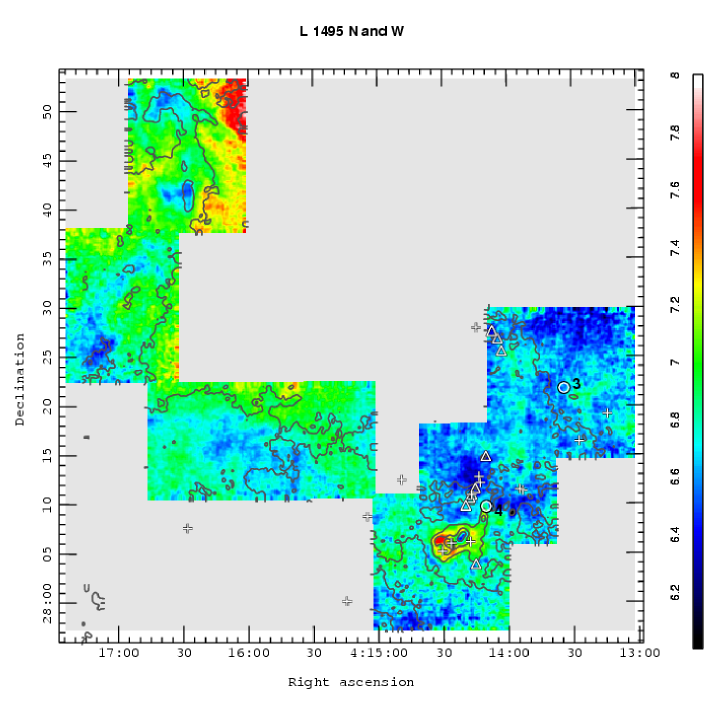
Figure 5: Same as Fig. 4 but for the region labelled L 1495 N and L 1495 W in Fig. 1. Again, there is CO 3-2 line emission throughout this region.

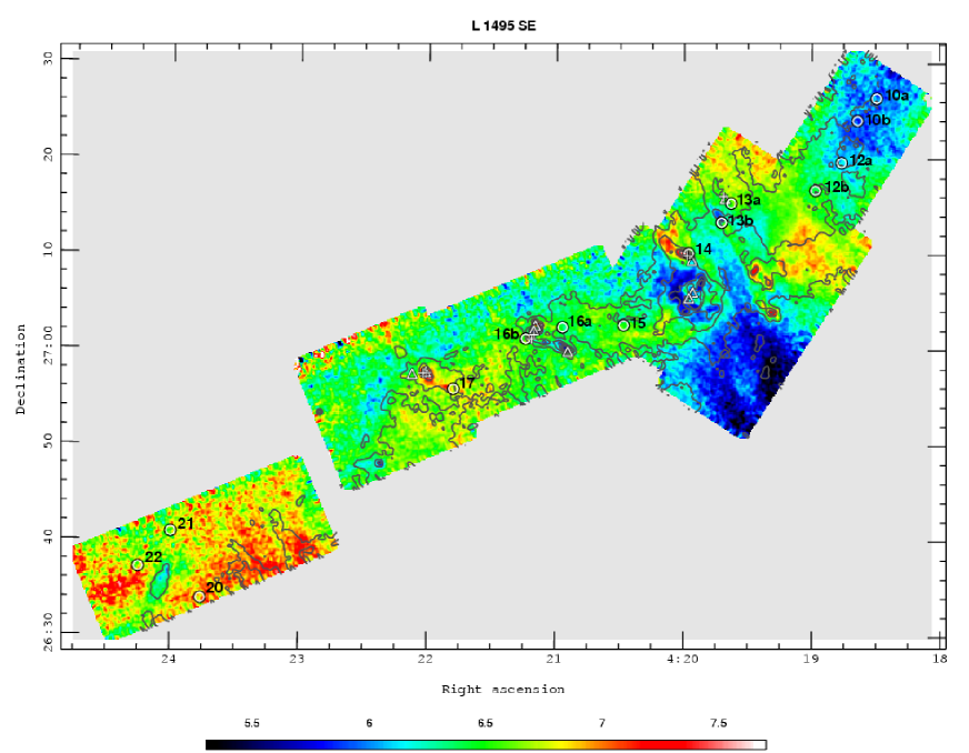
Figure 6: Same as Fig. 4 but for the SE ridge in L 1495. In this region the colours span 5.3  km s^-1 (black/blue) to 7.7  km s^-1 (red/white). Once again, we detect CO 3-2 line emission throughout this entire region.

To illustrate the velocity structure observed in CO 3-2, we present in Figs. 4–6 intensity-weighted radial velocity maps, colour-coded to show subtle changes in the centroid velocity of the gas (note that CO 3-2 line emission is detected at all locations in each image). These reveal the collimated blue- and red-shifted lobes of a number of outflows in L 1495, but also large-scale velocity gradients and “bubbles” of gas associated with clusters of young stars. In L 1495 E, for example, diffuse, red-shifted emission envelopes the cluster of YSOs to the east of the H¹³CO⁺ cores 5-8 (Fig. 4; the YSOs are marked with crosses in this figure). CO velocities to the west and south of this chain of cores are more blue-shifted (a result confirmed by the CO 1-0 observations of Goldsmith et al. 2008). The cluster of YSOs and the associated gas may be detaching itself from the rest of the cloud; alternatively, the red-shifted CO may represent a bubble being driven eastward by the cluster of young stars.

In L 1495 W, H¹³CO⁺ core 4 seems to be surrounded by a number of young stars; those to the north coincide with a region of blue-shifted CO, while those to the south coincide with a very distinct cloud of red-shifted gas (Fig. 5). T Tauri stars are often more widely distributed than their younger protostellar counterparts and prestellar cores; in L 1495 E and L 1495 W we may therefore be witnessing the expansion of the natal cloud and the dispersal of these young stars.

We also note the east-west velocity gradient seen in the L 1495 N region. The map in Fig. 5 suggests that the diffuse background emission to the north-west of the L 1495 bowl – in the unobserved regions in the centre and top of the figure – is likely to be red-shifted with respect to the denser material in the bowl. Again, this is evident in the CO 1-0 observations of Goldsmith et al. (2008).

Along the SE ridge, a number of collimated outflow lobes (discussed further below) are superimposed onto a ridge of diffuse CO. In the centre of Fig. 6 there is some indication that the south-west edge of the ridge is red-shifted with respect to the north-east edge. The cores and YSOs in this area lie predominantly along the boundary between this blue- and red-shifted gas. If the cores and young stars delineate the high-density axis of the L 1495 ridge, then this distribution of blue-shifted and red-shifted gas could be symptomatic of rotation.

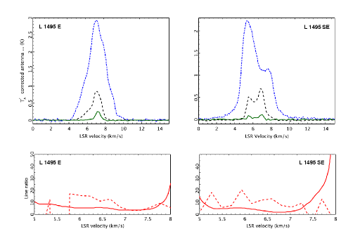
Figure 7: Top: ¹²CO 3-2 (blue/dot-dashed), ¹³CO 3-2 (black/dashed), and C¹⁸O 3-2 (green/full) spectra, averaged over the full extent of the areas mapped simultaneously in ¹³CO and C¹⁸O in L 1495 E and L 1495 SE. The ¹³CO and C¹⁸O spectra have been binned to a resolution of 0.25  km s^-1 ; the resolution of the ¹²CO 3-2 spectra is 0.05  km s^-1. Bottom: ratio of these averaged spectra; ¹²CO/¹³CO full red lines, ¹³CO/C¹⁸O dashed red lines.

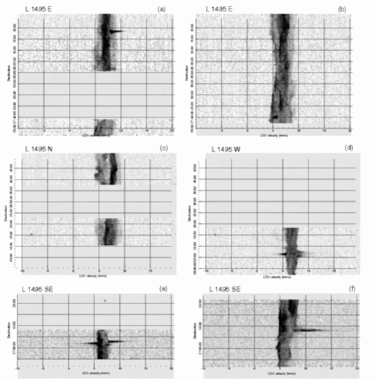
Figure 8: CO 3-2 position-velocity diagrams measured along vertical slices through L 1495 E at RA 4:18:14.2 (a) and RA 4:17:30.1 (b), through L 1495 N at RA 4:16:30.2 (c), through L 1494 W at RA 4:14:22.2 (d), and through L 1495 SE at RA 4:21:11.1 (e) and RA 4:19:28.7 (f).

3.2 Averaged spectra and PV diagrams

Averaged spectra and Position-Velocity (PV) diagrams are shown in Figs. 7 and 8. The former illustrate the relatively quiescent nature of the bulk of the gas in L 1495. They also give an indication of the mean opacity in the three lines observed. If the gas is optically thin then the line intensity ratios at a given velocity should approach the abundance ratios, X[¹²CO/¹³CO]=70 and X[¹³CO/C¹⁸O]=8.4 (Frerking, Langer & Wilson, 1982; Wilson, 1999), provided that the excitation temperature and beam efficiency and filling factors are the same for all three lines. Photo-dissociation and chemical fractionation effects in low-extinction regions can also lead to enhanced isotopic ratios (Langer et al., 1989). At intermediate velocities (5-8  km s^-1), where line emission is detected in all three isotopologues, the ¹³CO/C¹⁸O line ratio is indeed close to this canonical value (see lower panels in Fig. 7). However, at these velocities the ¹²CO/¹³CO ratio is of the order of 5-10, so the ¹²CO emission is clearly optically thick. For a ¹²CO/¹³CO abundance ratio of 70, the ¹²CO opacity, $\tau_{12}$, is given by:

$$\frac{\int T^{*}_{A}(^{12}{\rm CO}).\delta v}{\int T^{*}_{A}(^{13}{\rm CO}).\delta v}=\frac{(1-e^{-\tau_{12}})}{(1-e^{-\tau_{13}})}$$ (1)

where $\tau_{13}=\tau_{12}/70$. A ¹²CO/¹³CO line ratio of $\sim 10$ thus results in $\tau_{12}\sim 7.4$. Again, this value will be overestimated since ¹²CO is almost certainly self-absorbed; a lower abundance ratio (e.g. Goldsmith et al., 2008) would also result in a lower opacity. The ratio does increase towards blue-shifted and, particularly, red-shifted velocities. It therefore seems likely that, in the extended regions where the bulk of the outflowing gas is found, the high velocity line emission used to calculate the outflow parameters listed below will be only marginally optically thick.

PV diagrams, some of which are shown in Fig. 8, are useful for distinguishing compact molecular outflows from turbulent motions in the large-scale cloud. The outflows are seen as discrete horizontal spikes; turbulence appears as regions of diffuse emission that are more extensive along the spatial axis (vertically in these plots) though confined to low velocities, i.e. to within a few  km s^-1 of the ambient gas velocity. Indeed, we suggest that “eyeballing” outflows in PV diagrams is a relatively reliable way of finding them in HARP data cubes, since they are spatially (in one axis at least) as well as spectrally distinct from turbulent cloud motions and multiple cores seen along the same sight-line.

We have therefore searched for outflows by stepping through our data cubes in latitude and then in longitude, identifying spikes in PV space that extend more than $\pm$2.5  km s^-1 from the local ambient velocity with an intensity of $>$0.3 K (roughly the 2$\sigma$ level). A spike is defined as being narrower than 1′ in the spatial direction (i.e. in longitude and/or in latitude); we adopt 1′ as a conservative upper limit to the width of an outflow lobe. Outflows are subsequently verified in red-shifted and blue-shifted integrated intensity maps, most of which are presented in the next section.

A number of outflows are evident in Figs. 8. In the L 1496 E region, for example, a compact, red-shifted knot of emission $\sim$8′ to the west-south-west of CoKuTau-1, which we later refer to as E-CO-R1, is very distinct at declination $\sim$28^∘18′ in Fig. 8a. This feature is also evident $\sim$5′ south-east of core 7 in Fig. 4. Similar, though less extreme spikes extending red-ward and blue-ward of the ambient gas are seen to the north of V892 Tau (not shown, though discussed further below). Fig. 8b is typical of PV diagrams further west, toward the centre of the L 1495 bowl, where we find no clear-cut examples of molecular outflows, though where the gas generally appears more turbulent. This is particularly true in the region labelled L 1495 N in Fig. 1, where the emission profiles are double-peaked (top section in Fig. 8c). The CO 3-2 emission appears somewhat more ordered to the south and west of this region (see for example Fig. 8c [lower section] and Fig. 8d).

Along the south-eastern ridge in L 1495, PV spikes associated with high-velocity outflows are more prevalent. Example PV diagrams, again plotted along the declination axis, are presented in Fig. 8e and 8f: these show emission from the complex HH 392 region and the red lobe of the collimated bipolar outflow associated with IRAS 04166+2706 and core 13b, respectively (discussed further below).

3.3 Outflows in L 1495

When trying to identify outflows in complex regions like L 1495 one ideally needs a measure of the systemic velocity associated with each outflow driving source. This is difficult to do using the CO 3-2 observations alone (Fig. 8); even the ¹³CO and C¹⁸O profiles are double-peaked in some regions (Fig. 7). We therefore use the H¹³CO⁺ observations of OMK02 as a guide; these data are more likely to be optically thin and trace only the quiescent, high-density gas in each area. Cores are mapped throughout the bowl and south-east ridge in L 1495. The H¹³CO⁺ data also suggest that the ambient velocity does not change drastically across the region (Table LABEL:obs), a result which is supported by our CO 3-2 observations (particularly when one scans through the CO 3-2 data cubes in PV space), and our more optically thin, though less-extensive, ¹³CO and C¹⁸O data (Figs. 2 and 3).

When constructing integrated intensity maps of the high-velocity blue and red-shifted gas, we therefore adopt systemic velocities of 7.0 km s^-1, 6.7 km s^-1 and 6.6 km s^-1 for the L 1495 E, L 1495 W and L 1495 SE regions, respectively. Contour maps for select regions are presented in Figs. 9 - 12, where we also over-plot the positions of the Taurus YSOs, known HH objects and H¹³CO⁺ cores for reference.

In these figures we make use of shallow though extensive near-infrared images of Taurus, obtained as part of the U.K. Infrared Deep Sky Survey currently being conducted at the United Kingdom Infrared Telescope (UKIDSS: Lawrence et al., 2007). Images in broad-band K and narrow-band H₂ 2.122 $\mu$m emission (hereafter referred to simply as H₂) have been secured for the entire Taurus-Auriga-Perseus complex. The wide-field camera (WFCAM) used to obtain these data, the data reduction procedure, and the WFCAM archive are described in detail by Lucas et al. (2008) and Davis et al. (2008). Note that we also use the acronym “MHO” for the molecular hydrogen emission-line objects – the shock-excited infrared counterparts to HH objects – observed in L 1495. A complete catalogue of all known galactic MHOs is available on-line and in Davis et al. (2010).

Below we discuss the star forming regions in L 1495 individually.

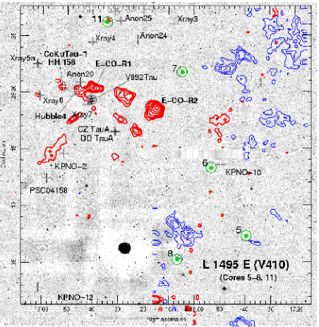
Figure 9: High-velocity CO 3-2 emission in L 1495 E, integrated between 4.0 and 6.0 km s^-1 (blue/thin contours) and 8.0 and 10.0 km s^-1 (red/thick contours), plotted as contours on top of a narrow-band H₂ ($+$ continuum) image of the region; contour levels are 1.75,2,2.5,3,4,5,7,10 K  km s^-1. Green circles, crosses and triangles mark H¹³CO⁺ cores, YSOs and HH objects, respectively.

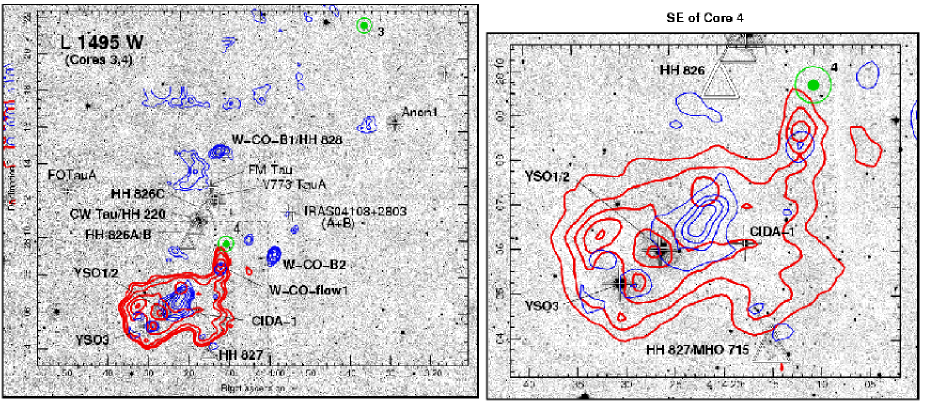
Figure 10: Same as Fig. 9 but for the L 1495 W region. Left - high-velocity CO 3-2 integrated between 3.7 and 5.7 km s^-1 (blue/thin contours) and 7.7 and 9.7 km s^-1 (red/thick contours). Contour levels are 1.0(blue-shifted only),1.2,1.5,2,3,4,5,7,10 K  km s^-1. Right - a close-up view of the region to the south-east of core 4 (marked with a dashed square at left); contours measure 1,2,3,4,5,7,10 K  km s^-1.

3.3.1 L 1495 E: CoKu Tau-1 and HH 156

L 1495 E harbours a cluster of about a dozen TTSs, many of which have been identified through X-ray observations (the V 410 X-ray and Anon# sources; Strom & Strom, 1994). OMK02 label five cores in this region. In the integrated intensity maps in Fig. 1 the CO is diffuse and optically thick across much of the region; only a few compact peaks are detected, all of which are marginally red-shifted and unrelated to the H¹³CO⁺ cores (Fig. 9, though note that the H¹³CO⁺ map does not cover the region south of the young star Xray 7 and east of core 8).

Two seemingly unrelated red-shifted knots are identified as molecular outflow features, E-CO-R1 and E-CO-R2. Neither is obviously related to any of the YSOs or H¹³CO⁺ cores; their progenitors remain unknown, although candidate sources surround E-CO-R1, and this object does coincide with a peak in our ¹³CO integrated intensity map in Fig. 1. Note also that in the H₂ images we detect no line-emission features in this region.

In Fig. 9 CoKu Tau-1 seems to be associated with a third compact red-shifted CO feature. However, this low-velocity knot of emission fails our search criteria for outflows (described above) and so is not identified as such here. CoKu Tau-1 does power HH 156 A and B, two compact HH objects offset $\sim$2″ and $\sim$12″ to the south-south-west; the CO peak could represent the counter-lobe, though deeper and/or higher-resolution CO data are needed to be sure. (The lack of blue-shifted CO around HH 156 may be a result of the HH flow exiting the cloud, or may be due to the dispersal of the core around this TTS.)

Apart from CoKu Tau-1, none of the young stars in the region are obviously driving CO outflows; presumably most are too evolved. Of the dozen YSOs to the east of cores 5-8 in Fig. 9, all bar three have neutral Spitzer-IRAC colours ([3.6]-[4.5]$\sim$0; [5.8]-[8.0]$\sim$0), consistent with relatively evolved (weak-line) TTSs and an absence of mid-infrared excess due to a lack of circumstellar material (Luhman et al., 2006, note that V 892 Tau is saturated). Only CoKu Tau-1, CZ TauA and DD Tau A have 2MASS near-IR and Spitzer mid-IR magnitudes that brighten towards longer wavelengths, consistent with them being protostars or very young T Tauri stars and therefore possible molecular outflow candidates. This low number of protostars in L 1495 E is consistent with the paucity of outflows in our H₂ and CO data.

3.3.2 L 1495 W: CW Tau and HH 220/826-828

The high-velocity CO in L 1495 W is shown in Fig. 10. Again, the positions of candidate YSOs are marked, although note that the Spitzer observations of Luhman et al. (2006) do not cover this region. The most dramatic feature in this area is the bubble of red-shifted gas that surrounds a small group of young stars, YSOs 1,2,3 and CIDA-1 (see also Fig. 5). More compact blue-shifted features are also observed in L 1495 W.

At least four molecular outflows exist in this region: (1) a compact north-south bipolar flow, W-CO-flow1, centred $\sim$1′ south of (and seemingly unrelated to) H¹³CO⁺ core 4, (2) a collimated blue-shifted lobe extending north-westward from YSOs 1 and 2 (which presumably also drive some [or all] of the red-shifted CO to the south-east), (3) a compact blue-shifted CO feature, W-CO-B1, associated with HH 828, and (4) a second blue CO knot, W-CO-B2, to the south-west of core 4, which may well be driven by IRAS 04108+2803A; this CO knot is certainly extended towards this object, which is also rather red (J-H = 3.10, H-K_s = 2.32).

Two additional flows are detected in HH and H₂ emission, HH 220/826, a jet from CW Tau (McGroarty & Ray, 2004), and an arc of HH/H₂ emission, HH 827/MHO 715, which may be associated with low-velocity red-shifted CO extending southward from CIDA-1 (though again this emission fails our outflow criteria).

YSO 1/2, YSO 3 and CIDA-1 have near-IR 2MASS colours consistent with youth. The TTSs CW Tau, V773 Tau A and FM Tau are more evolved and appear to be associated with a completely separate region of star formation. CW Tau is thought to be the most active classical TTS in this region. Even so, we detect no H₂ line emission from its HH objects, and only HH 828 appears to be associated with high-velocity (blue-shifted) CO emission.

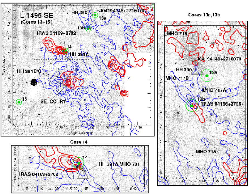
Figure 11: Same as Fig. 9 but for the region around cores 13-15 in L 1495 SE. Top-left - high-velocity CO 3-2 integrated between 3.6 and 5.6 km s^-1 (blue/thin contours) and 7.6 and 9.6 km s^-1 (red/thick contours); levels are 2,3,4,5,7,10 K  km s^-1 for both blue- and red-shifted emission. Right and Bottom-left - close-up views of the outflows associated with cores 13a,13b and 14: contour levels are 1.5(red only),2,3,4,5,7,10 K  km s^-1 in the former and 2,3,4,7,10 K  km s^-1 in the latter.

3.3.3 L 1495 SE: HH 390-391

The lower portion of the L 1495 ridge is populated with a number of young stars and HH flows. The area around cores 13a, 13b, 14 and 15 is shown in Fig. 11. Two of these four H¹³CO⁺ cores (13b and 14) are associated with IRAS sources and HH objects.

IRAS 04169+2702 (core 14) drives a collimated, possibly precessing bipolar molecular outflow and HH object (HH 391A); the HH object is also identified in H₂ emission, MHO 731 (see also Gomez et al., 1997).

A second, rather spectacular bipolar CO outflow emanates from core 13b. This flow is particularly striking in Fig. 6. The source of the outflow, IRAS 04166+2706, is identified at submm wavelengths (Santiago-García et al., 2009), though it does not appear in the 2MASS point source catalogue nor in the YSO lists of Luhman et al. (2006) and Kenyon et al. (2009). It must therefore be particularly young, as expected for molecular outflow and MHO progenitors (Hatchell et al. 2007b; Davis et al. 2008, 2009). Very faint H₂ features, MHO 717 A/B and MHO 718, are observed in both flow lobes. This outflow is well-known from previous CO observations: Tafalla et al. (2004) report the discovery of a collimated, Extremely High Velocity (EHV) outflow from IRAS 04166+2706, which Santiago-García et al. (2009) have since observed in SiO 2-1 emission. Both groups present CO 2-1 spectra with striking peaks in the line wings at -35  km s^-1 and +45  km s^-1. However, this EHV outflow component is only marginally detected (at the 2-3$\sigma$ level) in our 3-2 data. Based on a noise level of $T^{*}_{A}(rms)\sim 0.1$ K in our data (equivalent to a main beam brightness temperature of $\sim 0.2$ K), we set an upper limit of $\sim$0.5 for the 3-2/2-1 intensity ratio (note that the beam sizes are comparable). This ratio suggests that the clumps or “molecular bullets” associated with the EHV flow from IRAS 04166+2706 are relatively cold and/or diffuse ($n_{H2}\leq 10^{4}$ cm^-3, $T\leq 50$ K; Yeh et al., 2008).

Core 13a drives a much less well defined molecular outflow. MHO 716 may be associated with a red-shifted outflow lobe; HH 390 (which extends towards the south-west; Gomez et al., 1997) would then be excited in the blue lobe. The 2MASS source J04194148+2716070, which Luhman et al. (2006) and Kenyon et al. (2009) mis-identify as IRAS 04166+2706, is situated $\sim$50″ to the north-east of core 13a, and is a possible driving source for this outflow.

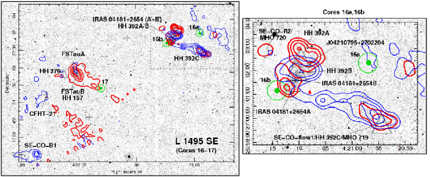
Figure 12: Same as Fig. 9 but for the region around cores 16a,16b and 17 in L 1495 SE. Left - high-velocity CO 3-2 integrated between 3.6 and 5.6 km s^-1 (blue/thin contours) and 7.6 and 9.6 km s^-1 (red/thick contours); levels are 1,2,3,4,5,7,10 K  km s^-1 for both blue- and red-shifted emission. Right - a close-up of the outflows associated with cores 16a and 16b; contour levels are 1,2,4,7,10 K  km s^-1.

Considering these three cores (13a, 13b and 14) and their associated YSOs together, IRAS 04166+2706 is presumably the youngest of the three; this is consistent with its powerful EHV CO outflow, its H₂ shocks, and the absence of HH objects. IRAS 04169+2702 is probably somewhat more evolved, having infrared colours that are consistent with a Class I protostar (H-K_s = 2.6; [3.6]-[5.8] = 2.1). J04194148+2716070 is bluer and is almost certainly a TTS, which would explain its association with an HH object and the lack of well-defined CO 3-2 outflow lobes.

Further south, HH 391 B and C represent a chain of optical features that extend over $\sim$1′ in a north-south direction (Gomez et al., 1997). These objects coincide with large, complex bubbles of both blue- and red-shifted emission. HH 391 B/C are unlikely to be associated with the IRAS 04169+2702/HH 391 A outflow. No H₂ emission was detected in this region, and the relationship between these shock features and the complex CO emission in this area is unclear, although high-velocity CO does coincide with these objects (we label the more clearly-defined red-shifted emission SE-CO-R1). Moreover, a ¹³CO peak does coincide with HH 391 B/C in our integrated intensity map in Fig. 1, which may be a sign of youth.

3.3.4 L 1495 SE: FS Tau A/B (Haro 6-5B) and HH 157/276/392

Moving further south-east along the L 1495 ridge, molecular outflows are detected around IRAS 04181+2654 and the well-studied FS Tau A/B (Haro 6-5B) system (Fig. 12).

IRAS 04181+2654 A is closest to core 16b and appears to drive a bipolar CO outflow in a roughly east-west direction. The blue lobe of this flow may overlap with a second bipolar outflow, SE-CO-flow1, which drives the compact shock features HH 392 C/MHO 719. There is no source candidate for SE-CO-flow1 in the 2MASS or IRAS point source catalogues, and Luhman et al. (2006) and Kenyon et al. (2009) do not identify a YSO near these objects. IRAS 04181+2654 A is resolved by 2MASS and exhibits an excess consistent with a protostar (J-H = 3.58, H-K_s = 2.30).

IRAS 04181+2654 B lies $\sim$30″ north-west of star A; this nebulous infrared source is associated with an arc of HH emission, HH 392 B (tentatively detected here in H₂) and also possesses considerable excess in the near-IR (J-H = 5.11, H-K_s = 2.70). The third source in the region, 2MASS source J04210795+2702204, has less extreme near-IR colours (J-H = 1.8, H-K_s = 1.5), though may nonetheless also contribute to the complex high-velocity CO evident in Fig. 12. The “kidney” shape of the blue- and red-shifted features coincident with HH 392 A and B certainly suggest the presence of multiple flow lobes.

Approximately 1.5′ to the north-east of IRAS 04181+2654 there is a faint knot of H₂ emission, MHO 720, which coincides with a knot of red-shifted CO, SE-CO-R2, and a very marginal detection of blue-shifted CO offset $\sim$15″ to the south-west. In all, there are at least four molecular outflows within a 5′ radius of cores 16a and 16b.

FS Tau A (J-H = 1.47, H-K_s = 1.73) and FS Tau B (J-H = 1.06, H-K_s = 1.60; also known as Haro 6-5B) are a pair of TTSs, the latter being associated with the spectacular HH jet and bow shock HH 157 (Eislöffel & Mundt, 1998). We detect red-shifted CO emission from this outflow, though no H₂ line emission. HH 276 is a chain of faint HH knots that crosses the HH 157 jet $\sim$1′ to the north-east of FS Tau B, although no high-velocity CO is clearly identified from this flow.

Lastly, south-east of FS Tau A, we note the very tentative detection of a bipolar CO outflow from CFHT-21, orientated NE-SW, roughly parallel with the FS Tau B jet. This marginal detection is consistent with the near-IR colours of this TTS (J-H = 1.5, H-K_s = 1.0). SE-CO-B1 is a compact though massive high-velocity knot with a tail extending along the south-east ridge. This feature is, however, not related to any known YSOs in the region.

Table 2: Parameters for the outflows in L 1495. The top nine flows are in the bowl; the remaining flows are in the south-east ridge.

YSO or Outflowa	Areaa	YSO	RAa	Dec a	CO flowb	HH/MHOc	H13CO+	$M$d	$|v_{o}-v|$d	$P^{d}$	$E^{d}$
		typea	(J2000.0)	(J2000.0)			corec	( M⊙)	km s-1	( M⊙	($\times 10^{34}$
										km s-1)	J)
CoKu Tau-1	E	TTS	4:18:51.5	28:20:26	No?	HH156		–	–	–	–
E-CO-R1e	E	–	4:18:39.5	20:20:20	Red			0.0098	2.3	0.022	5
E-CO-R2e	E	–	4:18:15.0	28:18:30	Red			0.0256	4.0	0.102	41
YSO 1/2	W	Class I	4:14:26.3	28:06:03	Bipolar			0.0156	4.7	0.074	35
CIDA-1	W	TTS	4:14:17.6	28:06:10	No?	HH827/MHO715		–	–	–	–
CW Tau	W	TTS	4:14:17.0	28:10:58	No?	HH220/826		–	–	–	–
W-CO-B1e	W	–	4:14:10.7	28:14:40	Blue	HH828		0.0028	3.1	0.009	3
W-CO-flow1e	W	–	4:14:12.0	28:08:30	Bipolar		4?	0.0038	3.1	0.012	4
IRAS 04108+2803A?	W	Class I	4:13:57.4	28:09:10	Blue			0.0055	3.3	0.018	6
J04194148+2716070	SE	TTS	4:19:41.5	27:16:07	No	HH390/MHO716	13a?	–	–	–	–
IRAS 04166+2706f	SE	Class 0?	4:19:42.4	27:13:24	Bipolar	MHO717/718	13b	0.0217	8.9	0.193	172
IRAS 04169+2702	SE	Class I	4:19:58.5	27:09:57	Red	HH391A/MHO731	14	0.0301	6.1	0.184	112
SE-CO-R1	SE	–	4:19:52.5	27:05:30	Red?	HH391B/C		0.0592	6.2	0.367	228
SE-CO-R2	SE	–	4:21:17.1	27:02:50	Red	MHO720		0.0021	2.6	0.005	1
J04210795+2702204	SE	Early TTS	4:21:08.0	27:02:20	Bipolar	HH392A		0.0157	5.4	0.085	46
IRAS 04181+2654A	SE	Class I	4:21:11.5	27:01:09	Red?		16b	0.0049	2.6	0.013	3
IRAS 04181+2654B	SE	Class I	4:21:10.4	27:01:37	?	HH392B	16b?	–	–	–	–
SE-CO-flow1e	SE	–	4:20:56.0	27:00:00	Bipolar	HH392C/MHO719		0.0153	3.2	0.049	16
FS Tau B	SE	Early TTS	4:22:00.7	26:57:32	Red	HH157		0.0209	4.9	0.102	50
CFHT-21g	SE	TTS	4:22:16.8	26:54:57	Bipolar?			–	–	–	–
SE-CO-B1e	SE	–	4:22:22.0	26:48:00	Blue			0.0251	3.8	0.095	36

^aThe most likely driving source of the CO outflow, the area in which it is found in L 1495, its YSO type (based on near- and/or mid-IR colours) and its coordinates.
If no YSO source is identified the label used for the CO outflow or high-velocity CO peak is given. The coordinates then refer to the approximate midpoint between
the bipolar lobes, or the peak in the CO emission if the flow is monopolar.
^bIndication of whether the CO outflow is bipolar or monopolar (with a red-shifted or blue-shifted lobe clearly defined). “No” in this column indicates that no CO
outflow was detected.
^cAssociated HH objects, MHOs and H¹³CO⁺ core (from OMK02).
^dThe mass, maximum radial velocity (the difference between the nominal ambient velocity and the velocity in the line wings at the 2$\sigma$ noise level); the momentum
and the kinetic energy of each outflow lobe. Mean values are quoted if the flow is bipolar
^eCO outflows with no clearly identified driving source.
^fDriving source not listed in the YSO catalogue of Luhman et al. (2006), Kenyon et al. (2009), or detected by 2MASS.
^gCO outflow only a marginal detection; requires confirmation with deeper observations.

3.4 Outflow parameters

The physical parameters for the molecular outflows described above are listed in Table LABEL:flows (we also list HH outflows not detected in high-velocity CO emission). The mass in the molecular outflow lobes (the mean of both lobes if the outflow is bipolar) is derived from the column density integrated across the extent of the high-velocity line wings, which in turn is calculated from the integrated antenna temperature, corrected for the main-beam efficiency (we assume a beam filling factor of unity), and an estimate of the CO 3-2 excitation temperature.

The excitation temperature, $T_{ex}$, in the ambient gas can be estimated from the peak temperature in the CO 3-2 line profiles, provided the gas is optically thick though not self-absorbed (Pineda, Caselli & Goodman, 2008; Buckle et al., 2010). However, $T_{ex}$ in the ambient gas is not necessarily the same as $T_{ex}$ in the entrained outflow gas, where the kinetic temperature may be higher and the gas is almost certainly compressed as it is swept up by the underlying jet and HH/MHO bow shocks (e.g. Hatchell et al., 1999; Davis et al., 2000a; Giannini, Nisini & Lorenzetti, 2001; Lee et al., 2002; van Kempen et al., 2009). We therefore adopt a somewhat higher value than is implied by (a) the average CO 3-2 spectra in Fig. 7 ($T^{*}_{A}\sim 3$ K; $T_{ex}\sim 11$ K), which include the more diffuse regions away from the central south-east ridge and star forming cores, or (b) the brightest spectra observed in L 1495 ($T^{*}_{A}\sim 17$ K; $T_{ex}\sim 35$ K). We instead use a value of 50 K, consistent with the range in excitation temperature derived from CO line ratios in other outflows – albeit assuming optically thin emission (e.g. Davis, Smith & Moriarty-Schieven, 1998; Hatchell et al., 1999; Davis et al., 2000a; van Kempen et al., 2009). The mass is in any case relatively insensitive to temperature, varying by only 40% over the temperature range 20-100 K (Hatchell et al., 2007a). Assuming an abundance of $X_{\rm CO}=10^{-4}$ (Frerking, Langer & Wilson, 1982; Wilson, 1999), the column density (in units of cm^-2) is then given by $N_{H2}=2.5\times 10^{19}(\int T^{*}_{b}dv)$, where the integrated line wings are in units of K  km s^-1 (Hatchell et al., 2007a). $\int T^{*}_{b}dv$ is measured from the integrated high-velocity blue-shifted and red-shifted outflow maps used to plot the contours in Figs. 9–12; the integrated flux measured in an ellipse that envelopes each outflow lobe is “sky subtracted” using the flux measured in an outer annulus (this eliminates diffuse red-shifted or blue-shifted gas not associated with the outflow); the derived column density is then scaled by the HARP beam size and the factor 1.3$\times m_{\rm H2}$ (where $m_{\rm H2}$ is the mass of an H₂ molecule) to give the mass in each outflow lobe.

We assume that the wings of the CO 3-2 emission are optically thin, so the values in Table LABEL:flows will be lower limits: the mass, $M$, momentum, $P$, and kinetic energy, $E$, are probably underestimated by a factor of 2-4 (Cabrit & Bertout, 1990; Hatchell et al., 2007a). Furthermore, the radial velocity, $|v_{o}-v|$ ($v$ is the velocity in the line wings where the emission reaches the 2$\sigma$ noise level; $v_{o}$ is the ambient velocity from Table LABEL:obs), used to calculate the momentum and energy, will also be underestimated, by a factor $1/{\rm sin}i$, where $i$ is the inclination angle with respect to the plane of the sky. Obviously for flows close to the plane of the sky this factor can be quite considerable, although flows with $i\gg$ 60^∘ will be difficult to detect in our CO observations; for an inclination angle of 60^∘ $P$ and $E$ will be underestimated by an additional factor of 2 and 4, respectively. Even so, the parameters listed in Table LABEL:flows are not unusual for outflows from low-mass young stars. They are marginally lower than (within an order of magnitude of) those typically observed for low-mass YSO outflows in Orion, Ophiuchus and Perseus (e.g. Knee & Sandell, 2000; Williams, Plambeck & Heyer, 2003; Arce & Sargent, 2006; Bussmann et al., 2007; Stanke & Williams, 2007).

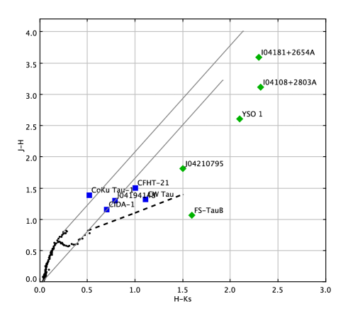
Figure 13: Near-IR colour-colour diagram for the HH jet and molecular outflow sources in L 1495, which are marked with blue squares and green diamonds, respectively. The black dots lower-left represent the locus of intrinsic colours for main sequence dwarfs and giants (Koornneef, 1983); the dashed line indicates the locus of T Tauri stars (Meyer, Calvet & Hillenbrand 1997). The full parallel lines are reddening vectors for the main sequence stars up to $A_{\rm v}=30$ mag (Rieke & Lebofsky, 1985).

4 Discussion

4.1 Using outflows to distinguish starless from protostellar cores in L 1495

L 1495 contains the largest concentration of young stars in the Taurus region. The majority of these are found in the L 1495 bowl, particularly the denser eastern half of the bowl (the molecular gas in the western bowl region is more extensive and generally more diffuse; Goldsmith et al., 2008) and in the lower half of the south-east ridge (Luhman et al., 2006; Kenyon et al., 2009). The low number-density of YSOs in the upper, north-western half of the ridge, where OMK02 nevertheless find a number of massive, dense cores (9a, 9b, 10a, 10b and 12), suggests that star formation has yet to take place in this area. The absence of HH objects, MHOs, and CO outflows in this region supports this interpretation.

The molecular outflows in L 1495 are listed in Table LABEL:flows, along with associated HH objects, MHOs, H¹³CO⁺ cores and candidate YSO driving sources. YSO source classifications are based on near-IR and/or mid-IR photometry (as described in section 1). In Fig. 13 we plot the 2MASS colours of the HH jet and outflow sources in Table LABEL:flows on a near-IR colour-colour (CC) diagram. As expected the majority of the sources lie to the right of the reddening band (the two parallel lines), although notably the sources with no CO outflow all lie in the region associated with TTSs, while the young stars that do drive molecular outflows are all much redder (in both J-H and H-K_s). Clearly the molecular outflow-driving sources are more embedded than their HH jet-driving counterparts.

Of the 22 cores labelled in Fig. 1 only four – 13a, 13b, 14 and 16b – appear to be associated with YSOs (in each case the YSO is located within the 50% integrated intensity contour in the H¹³CO⁺ maps). This relatively small fraction of cores with YSOs is consistent with the rest of Taurus; OMK02 find that only 22% of their condensations are associated with embedded sources. In L 1495 these “cores harbouring stars” certainly seem to be protostellar; at least three of the four cores (13b, 14 and 16b) are associated with molecular outflows; the CO flow from 13a is a marginal detection, though this core is also probably associated with an HH jet and MHO. As has been noted in other outflow surveys (e.g. Davis et al., 2008; Hatchell & Dunham, 2009), this suggests that CO outflows are useful tracers of the locations of protostellar cores. Indeed, outflow surveys may be used in combination with near- and mid-IR photometric studies of star forming regions to establish more accurately the fraction of cores that do harbour accreting protostars.

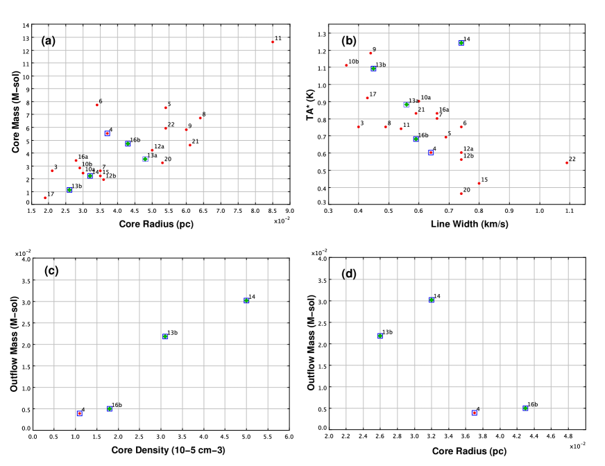
Figure 14: (a) Plot of H¹³CO⁺ core mass against core radius; (b) plot of H¹³CO⁺ line width against line intensity measured towards the peak in each core; (c) and (d) H¹³CO⁺ core molecular gas density and core radius plotted against the mass of the associated outflow. All core parameters are taken from Table 2 of OMK02. In each panel, cores are marked with red dots and are labelled according to OMK02; cores associated with YSOs are marked with green diamonds; cores associated with molecular outflows or HH jets are marked with open blue squares (note that we were unable to measure the molecular flow mass for core 13a).

Spitzer, when combined with near-IR data from e.g. 2MASS or WFCAM, can be a powerful tool for searching for Class 0/I protostars (although saturation can be a problem with Spitzer data, particularly at longer wavelengths). This is especially true in nearby, low mass star forming regions like Taurus, where extinction and crowding are minimal (Evans et al., 2009). A few recent studies have revealed the presence of extremely faint protostellar objects inside a handful of cores that were previously thought to be starless (Crapsi et al., 2005; Bourke et al., 2006). But such low-mass cores may be below the resolution and sensitivity limits of the H¹³CO⁺ survey discussed here, and these objects are unlikely to drive powerful CO outflows or bright H₂ jets. The YSO list, derived from optical, near-IR and mid-IR photometry and spectroscopy (Kenyon et al., 2009), is therefore expected to be relatively complete for the core mass range under scrutiny here.

A number of high-velocity CO features appear to be without driving sources in Table LABEL:flows. In some cases their progenitors may be nearby; however, in a few (W-CO-flow1, SE-CO-flow1, and SE-CO-R1/HH 391), the location of the driving source is clearly defined, yet they are still undetected. These flows are probably driven by Class 0 sources which require deeper mid-IR or far-IR/submm observations (Jørgensen et al., 2007, 2008).

From our comparison of the H¹³CO⁺ cores mapped by OMK02 to the YSO source list and outflows mapped here, at first sight the ratio of starless cores to protostellar cores in L 1495 seems to be high; as noted earlier, of the 22 cores located in L 1495, only 4 appear to be coincident with known YSOs (although all are associated with outflows).

However, two cores, 3 and 4, are found in a region that was not observed with Spitzer. Luhman et al. (2006) estimate that pre-Spitzer studies of the YSO population in Taurus are only complete to about 80% . They also point out that Spitzer is very well suited to finding disk-bearing stars down to masses of the order of 0.01  M_⊙ through considerable amounts of extinction ($A_{\rm v}\sim 100$). The observations of OMK02 are sensitive to core masses in the range 3.5 M_⊙ $<M<$ 20.1 M_⊙. Even for a very low star formation efficiency (low protostar-to-core mass ratio) of just a few percent (Ward-Thompson et al., 2007b), if these “starless” cores did contain protostars Spitzer would detect them. Given the small number statistics here, it is therefore possible that sensitive mid-IR observations could uncover protostars associated with both cores 3 and 4, in which case six of the 22 cores would be associated with protostars. (Note also that core 4 may be associated with the CO outflow W-CO-flow1.)

Hence, in L 1495 it seems reasonable to assume that we have 5$\pm$1 protostellar cores and 17$\pm$1 starless or prestellar cores; the ratio of cores that are associated with young stars to those that are not is in the range 0.2–0.4. But how many of the starless cores are prestellar? OMK02 and Mizuno et al. (1994) before them suggest that the fraction of H¹³CO⁺ cores in L 1495 that exceed the Jeans mass, are gravitationally bound, are undergoing some form of collapse, and therefore are prestellar in nature, is probably high: note that the H¹³CO⁺ cores identified by OMK02 are compact (radius $\leq 0.1$ pc) and of high density ($\geq 10^{5}$ cm^-3, the critical density for excitation of the H¹³CO⁺ line used in their study). They find that 13 of the 22 cores (60%) in L 1495 have an H¹³CO⁺ column density mass that exceeds the virial mass (these 13 include cores 3, 4, 13a, 13b and 16, i.e. five of the six candidate prestellar cores). This leads us to believe that 9 of the 22 are neither prestellar nor protostellar, so we identify these as being starless. The ratio of prestellar to protostellar cores in L 1495 is therefore in the range $\sim$1.3–2.3, while the ratio of starless to prestellar cores is in the range $\sim$1–1.3.

Although based on modest statistics, the above arguments indicate that the prestellar phase is about as long lived as the protostellar phase, and that in L 1495 there are as many prestellar cores as starless cores. Similar results have been found in Perseus (Hatchell et al., 2007a; Jørgensen et al., 2007; Hatchell & Fuller, 2008; Davis et al., 2008) and in other low mass star forming regions (Visser, Richer & Chandler, 2002; Enoch et al., 2007; Evans et al., 2009).

Evans et al. (2009) find the Class 0 lifetime to be $\sim$10⁵ yrs and the Class 0 and Class I lifetimes combined to be about 5 $\times$ 10⁵ yrs. It is worth mentioning that these timescales are more-or-less consistent with the range in dynamical ages, 10⁴ – 10⁵ yrs, measured for molecular outflows (Arce et al. 2007, and references therein); this is to be expected, given the statistical evidence that most protostars, particularly those associated with cores, drive molecular outflows (Davis et al., 2009).

Evans et al. (2009) also find the prestellar core lifetime to be of the order of 5$\times$10⁵ yr. OMK02, from their analysis of the data discussed here, estimate a very similar timescale ($\sim$ 4$\times$10⁵ yrs) for starless condensations in Taurus. If we assume a value of 5$\times$10⁵ yrs for the protostellar lifetime of our sources, then we arrive at a prestellar lifetime of $\sim$9($\pm$3)$\times$10⁵yrs. This is slightly longer than the timescale found by Evans et al., although it is still consistent to within the combined errors. Furthermore, we find the lifetime of starless cores that are not gravitationally bound to also be of the order of 10⁶ yrs.

4.2 The relationship between cores and outflows

OMK02 estimate various parameters for the H¹³CO⁺ condensations in Taurus, including size, density and mass. We plot a number of these in Fig. 14: in Fig. 14(a) we chart core mass based on the integrated intensity in H¹³CO⁺ emission against core radius (see OMK02 for details); a plot using the core virial mass, also calculated by OMK02, looks very similar to this figure. In Fig. 14(b) we plot the H¹³CO⁺ line width against H¹³CO⁺ peak antenna temperature; both have been measured by OMK02 at the peak position in each of their H¹³CO⁺ cores. Cores associated with embedded stars and outflows or HH jets are identified in both figures with green diamonds and open blue squares, respectively.

The plots in Fig. 14(a) and (b) suggest that the protostellar, outflow-driving cores are generally less massive, more compact and more quiescent than many of the observed condensations (although clearly not all of the compact H¹³CO⁺ cores are associated with outflows). At first glance this seems to run against expectation, since other studies have found that higher mass cores are more likely to be prestellar (e.g. Jørgensen et al., 2007; Hatchell & Fuller, 2008). However, one should note that the more massive H¹³CO⁺ cores are often larger (Fig. 14(a)) and less dense than their less massive counterparts; these objects may in fact harbour multiple, unresolved cores. Alternatively, these massive H¹³CO⁺ condensations may be younger than the protostellar cores, or may simply be gravitationally unbound and therefore not prestellar in nature.

For the H¹³CO⁺ cores that are associated with outflows and protostars, we find no correlation between core mass and outflow mass or kinetic energy (plots not shown). If anything, the more massive cores (4 and 16b) seem to be associated with the least massive flows. However, this comparison does not take into account the size of each core; Fig. 14(c) and (d) indicate a possible correlation between core density and outflow mass, and an inverse correlation between core size and outflow mass, albeit for a very small number of cores and outflows. The implication here is that the build-up of outflow mass increases as the protostellar core contracts. This idea clearly requires further investigation, both observationally and theoretically. Even so, our results are consistent with the early analysis of the H¹³CO⁺ data by Mizuno et al. (1994), who find that condensations with embedded stars in Taurus tend to be smaller in size, more dense, and less extended, than those without. Similar results were found in the submm continuum survey of Ward-Thompson et al. (1994).

Finally, we have conducted a statistical analysis of the data plotted in Fig. 14 (Isobe et al., 1990). This suggests that there is a 93% chance that the correlation between core mass and core radius is significant (i.e. there is a 7% chance that the sample is random), for cores with stars and for cores with outflows; for the entire sample there is a much higher chance ($>$99%) that the correlation is real, in part because of the much larger number of data points. Likewise, we find a $>$99% chance that for all cores the line intensity is related to the line width (Fig. 14(b)), although when only cores with stars or cores with outflows are considered the distribution of points is far less likely to be real ($\sim$65% and $<$50%, respectively). There is a 98.5% chance that the linear relationship between outflow mass and core density in Figs. 14(c) is real, though a reduced likelyhood (85%) that the distribution between outflow mass and core mass in Figs. 14(d) is significant. Strictly speaking, only the linear distribution of points in Figs. 14(c) is potentially real, although clearly both plots would benefit from additional data.

4.3 Star Formation Efficiency in L 1495 based on outflow statistics

In their study of outflow activity in Perseus-West, Davis et al. (2008) note that the more massive clouds are associated with a greater number of outflows. They use cloud masses derived from extinction mapping by Kirk, Johnstone & Di Francesco (2006), who note that this is arguably the best way of tracing the diffuse atomic and molecular gas ($A_{v}\sim 3-7$) in large molecular clouds. Kirk et al. also stress that only $\sim$5% of the cloud mass resides in regions with H₂ column densities $>5\times 10^{21}$ cm^-3 ($A_{v}>2.5$): in other words, only 5% of the gas mass is locked in the starless and protostellar cores mapped in H¹³CO⁺ and in submm dust continuum emission with, for example, SCUBA or SCUBA-2. Based on these measurements, in Perseus-West Davis et al. estimate that there is one outflow for every 44-88  M_⊙ of ambient material. This range is not inconsistent with a canonical value for the star formation efficiency ($SFE=M_{\rm YSO}$/[$M_{\rm YSO}+M_{\rm core}$]) of $\sim$10-15% (e.g. Jørgensen et al., 2007), if the cloud-to-core mass ratio is indeed $\sim$20, and the protostars have masses of the order of $\sim$0.5  M_⊙.

From their large-scale CO 2-1 and ¹³CO 2-1 observations of Taurus, Goldsmith et al. (2008) find that the L 1495 bowl and south-east ridge (regions they label L 1495 and B 213) have masses of the order of $2.6\times 10^{3}$  M_⊙ and $1.1\times 10^{3}$  M_⊙, respectively. Their observations are sensitive to H₂ column densities in excess of $\sim 1\times 10^{21}$ cm^-3 ($A_{v}>0.5$), so somewhat similar to the columns of molecular gas probed by the extinction mapping technique used in Perseus. In L 1495 we list (in Table LABEL:flows) nine outflows in the bowl and 12 in the L 1495 ridge; we therefore estimate roughly one outflow per 289 M_⊙ in the bowl, and one per 92  M_⊙ of gas in the ridge. These values are somewhat higher than in Perseus, especially in the bowl region. This is likely due to the more evolved state of this region, where the number of outflows underestimates the number of young stars and therefore the star formation efficiency. In the L 1495 bowl, a high percentage of young stars will be weak-line TTSs that are no longer associated with molecular or even HH flows. Note also that Taurus in general is considered to be a less active region of star formation, being associated with less luminous young stars, narrower molecular line widths and lower kinetic temperatures than e.g. Perseus or Orion (Jijina, Myers & Adams 1999).

4.4 Outflows, cloud structure and the large-scale B-field in L 1495

Taurus has been the subject of many studies of the large-scale cloud structure and its relationship to the surrounding magnetic field; Heyer (1988) and Goodman et al. (1992) measure the polarisation of background optical and infrared starlight via selective dust absorption, observations which illustrate the field orientation in the outer, low column density regions. Troland et al. (1996) and Crutcher & Troland (2000) present complementary Zeeman effect observations in 18 cm OH emission. Although these probe higher column densities, they only yield information on the line-of-sight field component, and are of lower (arcminute) spatial resolution. To better trace the B-field that pervades the dense cores and high-density gas that envelopes these cores, one requires high spatial resolution observations of polarised (sub)millimetre continuum emission from magnetically-aligned grains (e.g. Matthews, Wilson & Fiege, 2001; Matthews, Fiege & Moriarty-Schieven, 2002; Crutcher et al., 2004).

From studies of other low- and intermediate-mass star forming regions we know that the field orientation, projected onto the plane of the sky, often snakes through filaments and cores, changing direction on tenths of parsec scales (e.g. Davis et al., 2000b; Momose et al., 2001; Matthews & Wilson, 2002; Houde et al., 2002). Surveys of cores and clumps in star forming clouds also reveal a general lack of order in the orientations of the long axes of oblate starless and protostellar cores (e.g. Hatchell et al., 2005; Kirk et al., 2006); similarly, outflow surveys show that HH and H₂ line-emission jets are usually randomly orientated (Stanke, McCaughrean & Zinnecker, 2002; Walawender et al., 2005; Davis et al., 2009). Together, these data suggest that the magnetic field in the high-density regions is poorly coupled to the neutrals, allowing ambipolar diffusion to build up mass on star forming cores, or that the magnetic energy is insufficient to overcome the kinetic energy associated with the dense clumps and cores. Either way, the orientation of outflows and their associated protostellar cores do not appear to be strongly linked to the large-scale B-field.

But could L 1495 be an exception to the rule? The south-east ridge in L 1495 is notable for being orientated roughly perpendicular to the surrounding B-field (Goodman et al., 1992; Heiles, 2000; Goldsmith et al., 2008). Goodman et al. give a mean polarisation position angle along the ridge of 27^∘ from optical data, and 31^∘ from infrared polarisation measurements. Goldsmith et al. (2008) over-plot polarisation vectors (compiled by Heiles, 2000) onto their ¹³CO integrated intensity map of Taurus and find that the field is not only perpendicular to the L 1495 ridge, but is aligned with “striations” in the surrounding low column density medium. This suggests that – in these low density regions – the B-field is well coupled to the molecular gas through ion-neutral collisions (UV penetration maintaining a degree of ionisation in the gas). Collapse along these field lines may then produce the chain of high density condensations that forms the south-east ridge in L 1495. Although the field within the dense ridge awaits sensitive submm continuum polarisation measurements (these are planned as part of the Gould Belt survey), we point out here that many of the outflows found along the south-east ridge are orientated perpendicular to the ridge, and parallel with the field direction in the surrounding low column density gas. This observation is in general disagreement with the results of Greaves, Holland & Ward-Thompson (1997), who in a study of five protostars with outflows find that if the flow is in the plane of the sky the field tends to be orientated perpendicular to the flow axis. However, Greaves et al. used submm continuum polarisation measurements and therefore probed the higher column density regions close to each outflow source. It will be interesting to see whether the field direction, measured with the polarimetry facility currently being developed for SCUBA-2, changes close to the young outflow sources in L 1495.

5 Conclusions

HARP observations in CO 3-2 emission are shown to be ideal for tracing outflow activity in nearby star forming regions. The observations discussed here reveal as many as 16 molecular outflows in L 1495; most are associated with HH objects and/or molecular hydrogen line-emission features (MHOs). Candidate outflow driving sources (protostars or TTSs) are identified for eight CO flows, although only four of these flow progenitors appear to be associated with H¹³CO⁺ cores. Even so, we note that the CO outflow-driving sources have redder near-IR colours than their HH jet-driving counterparts. We also find a possible correlation between outflow mass and the associated core density and size, the more massive flows being associated with the denser, more compact cores.

OMK02 find that 13 of the 22 H¹³CO⁺ cores in L 1495 have a column-density mass that exceeds the virial mass. Of these 13 cores, five seem to be associated with protostars (and four of these drive outflows). We estimate that the ratio of prestellar to protostellar cores in L 1495 is approximately in the range 1.3–2.3; the ratio of starless to prestellar cores is estimated to be $\sim$1.

Overall, we find that the bowl is more evolved than the south-east ridge in L 1495; in the bowl there is a paucity of molecular flows though a larger fraction of TTSs. The fact that the ridge is spatially more compact (long and narrow) in comparison to the bowl supports this interpretation. The star formation efficiency in L 1495 (particularly the south-east ridge), estimated from the ambient cloud density, a canonical value for the cloud-to-core mass ratio, and the observed number of outflows, is consistent with other low-mass star forming regions.

In comparison to Orion and Perseus there is a modest number of outflows and protostars in L 1495. However, the region, especially the south-east ridge, is relatively simple (in comparison to, say, NGC 1333), with little chance for source confusion and outflows overlapping other outflows or unrelated molecular cores. The statistics, though modest, are therefore likely to be more robust than in other regions.

References

- Arce & Sargent (2006) Arce H.E., Sargent A.I., 2006, ApJ, 646, 1070
- Arce et al. (2007) Arce H., Shepherd D., Gueth F., Lee C.F., Bachiller R., Rosen A., Beuther H., 2007, in Protostars and Planets V, ed. B. Reipurth (Univ. Arizona Press: Tucson), p.245
- Bourke et al. (2006) Bourke T.L. et al., 2006, ApJ, 649, L37
- Buckle et al. (2010) Buckle J.V. et al., 2010, MNRAS, 401, 204
- Buckle et al. (2009) Buckle J.V. et al., 2009b, MNRAS, 399, 1026
- Bussmann et al. (2007) Bussmann R.S., Wong T.W., Hedden A.S., Kulesa C.A., Walker C.K., 2007, ApJ, 657, L33
- Cabrit & Bertout (1990) Cabrit S., Bertout C., 1990, ApJ, 349, 530
- Cavanagh et al. (2008) Cavanagh B., Jenness T., Economou F., Currie M.J., 2008, in Astronomische Nachrichten, 329, 295
- Crapsi et al. (2005) Crapsi, A. et al., 2005, A&A, 439, 1023
- Crutcher et al. (2004) Crutcher R.M., Nutter D., Ward-Thompson D., Kirk J.M., 2004, ApJ, 600, 279
- Crutcher & Troland (2000) Crutcher R.M., Troland T.H., 2000, ApJ, 537, L139
- Curtis et al. (2010) Curtis E.I., Richer J.S., Buckle J.V., 2010, MNRAS, 401, 455
- Davis et al. (2000b) Davis C.J., Chrysostomou A., Matthews H.E., Jenness T., Ray T.P., 2000b, ApJ, 530, L115
- Davis et al. (2000a) Davis C.J., Dent W.R.F., Matthews H.E., Coulson I.M., McCaughrean M.J., 2000a, MNRAS, 318, 952
- Davis et al. (2010) Davis C.J., Gell R., Khanzadyan T., Smith M.D., Jenness T., 2010, A&A, in press.
- Davis et al. (2008) Davis C.J., Scholz P., Lucas P.W., Adamson A., 2008, MNRAS, 387, 954
- Davis, Smith & Moriarty-Schieven (1998) Davis C.J., Smith M.D., Moriarty-Schieven G.H., 1998, MNRAS, 387, 954
- Davis et al. (2009) Davis C.J. et al. 2009, A&A, 496, 153
- Di Francesco et al. (2007) Di Francesco J., Evans II, N.J., Caselli P., Myers P.C., Shirley Y., Aikawa Y., Tafalla M., 2007, in Protostars and Planets V, ed. B. Reipurth (Univ. Arizona Press: Tucson), p.17
- Di Francesco et al. (2008) Di Francesco J., Johnstone D., Kirk H., MacKenzie T., Ledwosinska E., 2008, ApJS, 175, 277
- Dobashi et al. (2005) Dobashi K., Uehara H., Kandori R., Sakurai T., Kaiden M., Umemoto T., Sato F., 2005, PASJ, 57, 1
- Eislöffel & Mundt (1998) Eislöffel J., Mundt R., 1998, AJ, 115, 155
- Elias (1978) Elias J.H., 1978, ApJ, 224, 857
- Enoch et al. (2007) Enoch M.L., Glenn J., Evans N. J., Sargent, A.I., Young K.E., Huard T.L. 2007, ApJ, 666, 982
- Evans et al. (2009) Evans N.J. et al., 2009, ApJS, 181, 321
- Frerking, Langer & Wilson (1982) Frerking M.A., Langer W.D., Wilson R.W., 1982, ApJ, 262 590
- Giannini, Nisini & Lorenzetti (2001) Giannini T., Nisini B, Lorenzetti D., 2001, ApJ, 555, 40
- Goldsmith et al. (2008) Goldsmith P.F., Heyer M.H., Narayanan G., Snell R., Li D., Brunt C., 2008, ApJ, 680, 428
- Gómez de Castro (1993) Gómez de Castro A.I., 1993, ApJ, 412, L43
- Gomez et al. (1997) Gomez M., Whitney B.A., Kenyon S.J., 1997, AJ 114, 1138
- Gottlieb & Upson (1969) Gottlieb D.M., Upson W.L., 1969, ApJ, 157, 611
- Goodman et al. (1992) Goodman A.A., Jones T.J., Lada E.A., Myers P.C., 1992, ApJ, 399, 108
- Graves et al. (2010) Graves S.F. et al., 2010, MNRAS, submitted.
- Greaves et al. (1997) Greaves J.S., Holland W.S., Ward-Thompson D., 1997, ApJ, 480, 255
- Hatchell et al. (2005) Hatchell J. et al., 2005, A&A, 440, 151
- Hatchell & Dunham (2009) Hatchell J., Dunham M.M., 2009, A&A, 502, 139
- Hatchell et al. (1999) Hatchell J., Fuller G.A., Ladd E.F., 1999, A&A, 346, 584
- Hatchell & Fuller (2008) Hatchell J., Fuller G.A., 2008, A&A, 482, 855
- Hatchell et al. (2007a) Hatchell J., Fuller G.A., Richer J.S., 2007a, A&A, 472, 187
- Hatchell et al. (2007b) Hatchell J., Fuller G.A., Richer J.S., Harries T., Ladd E.F., 2007b, A&A, 468, 1009
- Hartmann et al. (2005) Hartmann L., Megeath S.T., Allen L., Luhman K., Calvet N., D’Alessio P., Franco-Hernandez R., Fazio G., 2005, ApJ, 629, 881
- Heiles (2000) Heiles C., 2000, AJ, 119, 923
- Heyer (1988) Heyer M.H., 1988, ApJ, 324, 311
- Holland et al. (2006) Holland W.S. et al., 2006, in Zmuidzas J., Holland W. S., Withington S. Duncan W.D., eds, Proc. SPIE Vol. 6275, SCUBA-2: a 10,000-pixel submillimeter camera for the James Clerk Maxwell Telescope, SPIE, p. 45
- Houde et al. (2002) Houde M. et al., 2002, ApJ, 569, 803
- Hovey et al. (2000) Hovey G.J. et al., 2000, in Butcher H. R., ed., SPIE Proc. Vol. 4015, Radio Telescopes. SPIE Bellingham, p. 114
- Isobe et al. (1990) Isobe T., Feigelson E.D., Akritas M.G., Babu G.J., 1990, ApJ, 364, 104
- Jenness et al. (2008) Jenness T., Cavanagh B., Economou F., Berry D.S., 2008, in ASP Conf. Ser., 394, 565
- Jijina et al. (1999) Jijina J., Myers P.C., Adams F.C., 1999, ApJS, 125, 161
- Jørgensen et al. (2006) Jørgensen J.K. et al. 2006, ApJ, 645, 1246
- Jørgensen et al. (2007) Jørgensen J.K., Johnstone D., Kirk H., Myers P.C., 2007, ApJ, 656, 293
- Jørgensen et al. (2008) Jørgensen J.K., Johnstone D., Kirk H., Myers P.C., Allen L.E., Shirley Y.L., 2008, ApJ, 683, 822
- Kenyon et al. (2009) Kenyon S.J., Gómez M., Whitney B.A., 2009, in Handbook of Star Forming Regions Vol.1, ed. B. Reipurth, ASP monographs, p.405
- Kenyon & Hartmann (1995) Kenyon S.J., Hartmann L., 1995, ApJS, 101, 117
- Kirk et al. (2006) Kirk H., Johnstone D., Di Francesco J., 2006, ApJ, 646, 1009
- Koornneef (1983) Koornneef J., 1983, A&A, 128, 84
- Knee & Sandell (2000) Knee L.B.G., Sandell G., 2000, A&A, 361, 671
- Langer et al. (1989) Langer W.D., Wilson R.W., Goldsmith P.F., Beichman C.A., 1989, ApJ, 337, 355
- Lawrence et al. (2007) Lawrence A. et al., 2007, MNRAS, 379, 1599
- Lee et al. (2007) Lee C.-F., Ho P.T.P., Palau A., Hirano N., Bourke T.L., Shang H., Zhang Q., 2007, ApJ, 670, 1188
- Lee et al. (2002) Lee C.-F., Mundy L.G., Stone J.M., Ostriker E.C., 2002, ApJ, 576, 294
- Lucas et al. (2008) Lucas P.W. et al., 2008, MNRAS, MNRAS, 391, 136
- Luhman et al. (2006) Luhman K.L., Whitney B.A., Meade M.R., Babler B.L., Indebetouw R., Bracker S., Churchwell E.B., 2006, ApJ, 647, 1180
- Matthews et al. (2008) Matthews H.E., McCutcheon W.H., Kirk H., White G.J., Cohen M., 2008, AJ, 136, 2083
- Matthews, Fiege & Moriarty-Schieven (2002) Matthews B.C., Fiege J.D., Moriarty-Schieven G.H., 2002, ApJ, 569, 304
- Matthews, Wilson & Fiege (2001) Matthews B.C., Wilson C.D., Fiege J.D., 2001, ApJ, 562, 400
- Matthews & Wilson (2002) Matthews B.C., Wilson C.D., 2002, ApJ, 574, 822
- McCuskey (1939) McCuskey S.W., 1939, ApJ, 89, 568
- McGroarty & Ray (2004) McGroarty F., Ray T.P., 2004, A&A, 420, 975
- Meyer et al. (1997) Meyer M.R., Calvet N., Hillenbrand L.A., 1997, AJ, 109, 1682
- Mizuno et al. (1994) Mizuno A., Onishi T., Hayashi M., Ohashi N., Sunada K., Hasegawa T., Fukui Y., 1994, Nature, 368, 719
- Mizuno et al. (1995) Mizuno A., et al. 1995, ApJ, 445, L16.
- Momose et al. (2001) Momose M., Tamura M., Kameya O., Greaves J.S., Chrysostomou A., Hough J.H., Morino J.I., 2001, ApJ, 555, 855
- Motte & André (2001) Motte F., André P., 2001, A&A, 365, 440
- Narayanan et al. (2008) Narayanan G., Heyer M.H., Brunt C., Goldsmith P.F., Snell R., Li D., 2008, ApJS, 177, 341
- Onishi et al. (1996) Onishi T., Mizuno A., Kawamura A., Ogawa H., Fukui Y., 1996, ApJ, 465, 815
- Onishi et al. (2002) Onishi T., Mizuno A., Kawamura A., Tachihara K., Fukui Y., 2002, ApJ, 575, 950 (OMK02)
- Pineda, Caselli & Goodman (2008) Pineda J.E., Caselli P., Goodman A.A., 2008, ApJ, 679, 481
- Racine (1968) Racine R., 1968, AJ, 73, 233
- Rieke & Lebofsky (1985) Rieke G.H., Lebofsky M.J., 1985, ApJ, 288, 618
- Santiago-García et al. (2009) Santiago-García J., Tafalla M., Johnstone D., Bachiller R., 2009, A&A, 495, 169
- Smith et al. (2003) Smith H., et al., 2003, Proc. SPIE, 4855, 338
- Stanke, McCaughrean & Zinnecker (2002) Stanke T., McCaughrean M.J., Zinnecker H., 2002, A&A, 392, 239
- Stanke & Williams (2007) Stanke T., Williams J.P., 2007, AJ, 133, 1307
- Strom & Strom (1994) Strom K.M., Strom S.E., 1994, ApJ, 424, 237
- Tafalla et al. (2002) Tafalla M. et al., 2002, ApJ, 569, 815
- Tafalla et al. (2004) Tafalla M., Santiago J., Johnstone D., Bachiller R., 2004, A&A, 423, L21
- Tatematsu et al. (2004) Tatematsu K., Umemoto T., Kandori R., Sekimoto Y., 2004, ApJ, 606, 333
- Torra, Fernández & Figueras (2000) Torra J., Fernández D., Figueras F., 2000, A&A, 359, 82
- Torres et al. (2009) Torres R.M., Loinard L., Mioduszewski A.J., Rodr guez L.F., 2009, ApJ, 698, 242
- Troland et al. (1996) Troland T.H., Crutcher R.M., Goodman A.A., Heiles C., Kazes I., Myers P.C., 1996, ApJ, 471, 302
- Ungerechts & Thaddeus (1987) Ungerechts H., Thaddeus P., 1987, ApJSS, 63, 645
- van Kempen et al. (2009) van Kempen T.A., et al. (13 authors), 2009, A&A, 501, 633
- Visser, Richer & Chandler (2002) Visser A.E., Richer J.S., Chandler C.J. 2002, AJ, 124, 2756
- Walawender et al. (2005) Walawender J., Bally J., Kirk H., Johnstone D., 2005, AJ, 130, 1795
- Ward-Thompson et al. (2007b) Ward-Thompson D., André P., Crutcher R., Johnstone D., Onishi T., Wilson C., 2007b, in Protostars and Planets V, ed. B. Reipurth (Univ. Arizona Press: Tucson), p.33
- Ward-Thompson et al. (1994) Ward-Thompson D., Scott P.F., Hills R.E., André P., 1994, MNRAS, 268, 276
- Ward-Thompson et al. (2007a) Ward-Thompson D., et al., 2007a, PASP, 119, 855
- Williams, Plambeck & Heyer (2003) Williams J.P., Plambeck R.L., Heyer M.H., 2003, ApJ, 591, 1025
- Wilson (1999) Wilson T.L., 1999, Rep. Prog. Phys., 62, 143
- Yeh et al. (2008) Yeh S.C.C., Hirano N., Bourke T.L., Ho P.T.P., Lee C-.F., Ohashi N., Takakuwa S., 2008, ApJ, 675, 454