The Effect of Star Spots on Accurate Radius Determination of
the Low Mass Double-lined Eclipsing Binary GU Boo

Abstract

GU Boo is one of only a relatively small number of well studied double-lined eclipsing binaries that contain low-mass stars. López-Morales & Ribas (2005, hereafter LR05) present a comprehensive analysis of multi-color light and radial velocity curves for this system. The GU Boo light curves presented in LR05 had substantial asymmetries, which were attributed to large spots. In spite of the asymmetry LR05 derived masses and radii accurate to $\simeq$ $2\%$. We obtained additional photometry of GU Boo using both a CCD and a single-channel photometer and modeled the light curves with the $\rm ELC$ software to determine if the large spots in the light curves give rise to systematic errors at the few percent level. We also modeled the original light curves from LR05 using models with and without spots. We derived a radius of the primary of $0.6329\pm 0.0026\,R_{\odot}$, $0.6413\pm 0.0049\,R_{\odot}$, and $0.6373\pm 0.0029\,R_{\odot}$ from the CCD, photoelectric, and LR05 data, respectively. Each of these measurements agrees with the value reported by LR05 ($R_{1}=0.623\pm 0.016\,R_{\odot}$) at the level of $\approx 2\%$. In addition, the spread in these values is $\approx 1-2\%$ from the mean. For the secondary, we derive radii of $0.6074\pm 0.0035\,R_{\odot}$, $0.5944\pm 0.0069\,R_{\odot}$, and $0.5976\pm 0.0059\,R_{\odot}$ from the three respective data sets. The LR05 value is $R_{2}=0.620\pm 0.020\,R_{\odot}$, which is $\approx 2-3\%$ larger than each of the three values we found. The spread in these values is $\approx 2\%$ from the mean. The systematic difference between our three determinations of the secondary radius and that of LR05 might be attributed to differences in the modelling process and codes used. Our own fits suggest that, for GU Boo at least, using accurate spot modelling of a single set of multicolor light curves results in radii determinations accurate at the $\approx 2\%$ level.

– : binaries: eclipsing; binaries: spectroscopic; stars: fundamental parameters; stars: individual (GU Boötis); stars: late-type; stars: spots

1 Introduction

Understanding the structure and evolution of stars is a basic goal of stellar astrophysics, and is also required in most other branches of astrophysics. Detailed models of stellar evolution can predict (among other things) the stellar radius as a function of mass and age. The Sun can be used to calibrate stellar evolution models since its mass, radius, and age are well determined (e.g., Guenther et al. 1992). Critical tests of evolution theory for stars other than the Sun can be made on a small set of eclipsing binary stars (e.g., Pols et al. 1997; Schröder et al. 1997). For this purpose, it is essential to derive accurate masses and radii for these binaries.

In general, the results of stellar evolution models compare favorably to data for main sequence stars with masses $\gtrsim 1\,M_{\odot}$ (e.g. Pols et al. 1997). However, the models for stars on the lower main sequence have problems matching precise data from eclipsing binaries. A good example is the double-lined eclipsing M-star binary YY Gem, which is a member of the Castor group. This binary contains a pair of nearly identical stars with masses of $M=0.599\,M_{\odot}$. Torres & Ribas (2002) have shown that all models for stars on the lower main sequence underestimate the radii of the YY Gem components by up to 20% and that most models overestimate the effective temperatures by 150 K or more. Similar trends are found in V818 Tau (Torres & Ribas 2002), CU Cnc (Ribas et al. 2003), GU Boo (López-Morales & Ribas 2005), TrES-Her0-07621 (Creevey et al.  2005), 2MASS J05162881+2607387 Schuh et al. 2003; Bayless & Orosz, 2006), NSVS 02502726 (Çakirli et al. 2009), and GJ 3236 (Irwin et al. 2009). The disagreement between the models and the data for these binaries is very troubling since models for low-mass stars are often used to estimate the ages for open clusters and for individual T Tauri stars by placing them in an H-R diagram. There have been recent suggestions that unusually strong stellar activity in these low-mass stars might make them larger than they otherwise would be (Ribas 2006; Torres et al. 2006; López-Morales 2007; Chabrier et al. 2007), and that the changes in the stars caused by stellar activity has not been properly accounted for in the evolutionary models.

In this paper, we focus on GU Boo. The GU Boo light curves presented by López-Morales & Ribas (2005, hereafter LR05) are very precise, which allowed them to derive radii accurate to a few percent using the well-known Wilson & Devinney (1971, W-D) code. However, their light curves are not symmetric about the primary eclipse. The system is brighter just before the secondary eclipse (i.e., at first contact) than it is just after the secondary eclipse (i.e., at fourth contact). The source of the excess light before secondary eclipse was attributed by LR05 to a bright spot and a larger dark spot on the primary. Although the W-D code can include spots, the spot model is somewhat simplistic (e.g., one or two circular regions with a different temperature than the rest of the star) and one has to wonder if the spots cause systematic errors in the fitting at the few percent level. One simple test of the robustness of the GU Boo parameters given by LR05 is to obtain new light curves and model all data independently. In what follows, we present new CCD and photoelectric observation of GU Boo obtained using the 1m telescope at Mount Laguna Observatory. In addition, the radial velocities published by LR05 and the light curves were kindly sent to us by Mercedes López-Morales. We model our new light curves and the LR05 light curves using various assumptions about the spots and compare our results with those of LR95. We end with a brief discussion and summary.

2 OBSERVATIONS

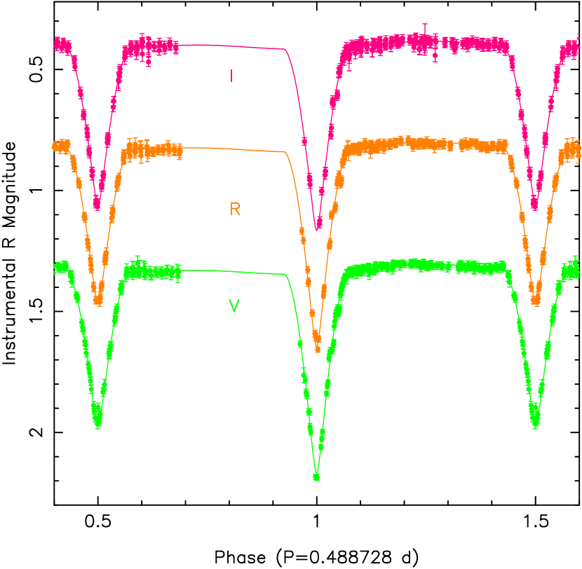
Figure 1: The CCD light curves of GU Boo obtained from Mount Laguna for the $V$, $R$, and $I$ filters and the best-fitting ELC model.

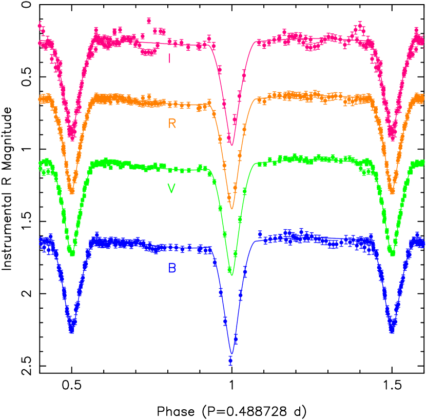
Figure 2: The photoelectric light curves of GU Boo obtained from Mount Laguna for the $V$, $R$, and $I$ filters and the best-fitting ELC model. The $I$-band light curve is somewhat noisy owing to a much higher level of background light.

We observed GU Boo during May-June of 2005 using the 1m telescope at the Mount Laguna Observatory. GU Boo was observed with a Fairchild CCD 447, backside illuminated $2048\times 2048$ with 15 micron square pixels, and $V$, $R$, and $I$ filters. Other data were taken with a single-channel photometer, employing an RCA C31034A GaAs based photomultiplier, and $B$, $V$, $R$, and $I$ filters (Bessell 1990). Table 1 gives a summary of the observations. Standard CCD image reductions were done in IRAF. The differential light curves of GU Boo were derived using simple aperture photometry in IRAF, including Stetson’s curve-of-growth technique (Stetson 1990) to derive optimal instrumental magnitudes corresponding to the largest aperture. The reductions for the photoelectric data (hereafter PMT) were done with the code FOTOM, which was developed at San Diego State University. The new CCD light curves are shown in Figure 1. The PMT light curves are shown in Figure 2.

3 METHOD AND RESULTS

3.1 Light Curve Comparison

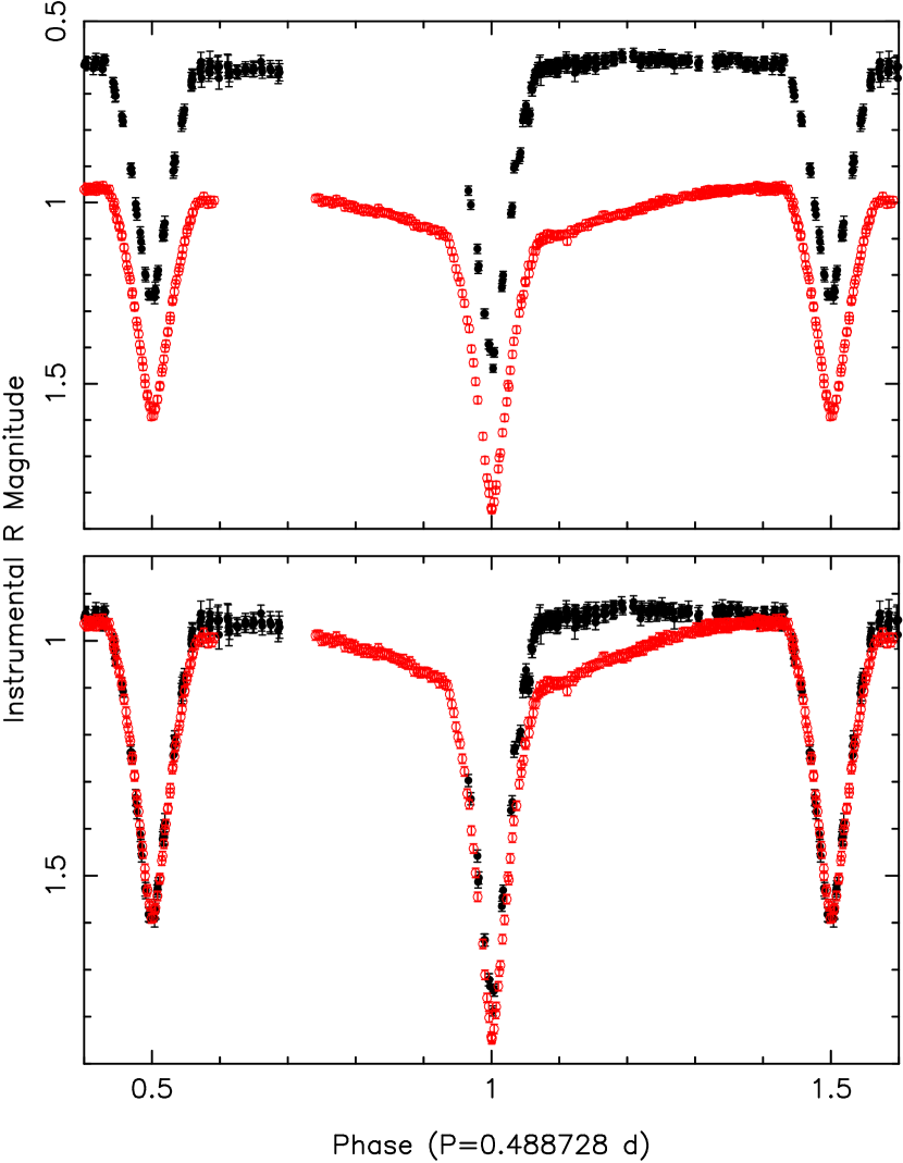
Figure 3: Bottom: A comparison of $R$-band data of GU Boo. The light curve from LR05 is shown with the red open circles. The CCD light curve obtained from Mount Laguna is shown with the black filled circles. Top: Same as the bottom, but with the light curves offset for clarity.

Figure 3 compares our $R$-band CCD light curve with the $R$-band light curve from LR05. The light curves are rather different. As noted above, the light curve from LR05 has a relatively large amount of variation in the out-of-eclipse phases, exhibiting two different slopes on either side of the primary eclipse. In contrast, the light curves from Mount Laguna are relatively flat between eclipses and are more symmetric. The secondary eclipse profiles are very similar, whereas the primary eclipse, as well as the nearby phases, are depressed to fainter levels in the LR05 light curve. The natural interpretation is that there was a rather large and dark spot on the primary when LR05 obtained their data, and that spot had mostly vanished by the time we observed the system from Mount Laguna. Indeed, LR05 invoked a large dark spot on the primary in their light curve modeling. The source changed relatively little in the few weeks between the CCD observations and the photoelectric observations (see Figures 1 and 2), making the spot(s) stable on a time-scale of a few weeks, which simplifies the light curve modeling discussed below. As shown here, the existence and asymmetry of spots on either the primary, the secondary, or both, can explain the differences between the two light curves in both the asymmetry and the non-zero derivative outside of eclipses.

3.2 Light Curve Modeling

We modeled our GU Boo light curves using our ELC code (Orosz & Hauschildt 2000) with updated model atmospheres for low mass stars and brown dwarfs (Hauschildt, private communication). As noted above, the radial velocities published by LR05 and the light curves were kindly sent to us by Mercedes López-Morales, and we included the radial velocities in all of our modeling runs. The CCD light curves were modeled separately from the PMT light curves. Using ELC’s various optimizers, we fit for the following 13 parameters (the ranges searched are given in parentheses): the primary mass $M_{1}$ ($0.5-0.7\,M_{\odot}$), the primary radius $R_{1}$ ($0.57-0.67\,R_{\odot}$), the ratio of the radii $R_{1}/R_{2}$ ($0.9-1.1$), the inclination $i$ ($75-90^{\circ}$), the $K$-velocity of the primary $K_{1}$ ($130.0-155.0$ km s^-1), the effective temperatures $T_{1}$ ($3700-3900$ K) and $T_{2}$ ($3600-3800$ K), the orbital period $P$ ($0.48871-0.48874$ d), the time of primary eclipse $T_{0}$ (HJD $2,452,723.98-2,452,723.99$), and 4 parameters to describe a spot, namely the “temperature factor” ($0.5-2.0$), the latitude ($0-180^{\circ}$), the longitude ($0-360^{\circ}$), and the angular radius ($0-60^{\circ}$). The mass ratio $Q$, and the semi-major axis $a$ are mapped to directly from the fitted parameters $M_{1}$ and $K_{1}$. We also modeled the LR05 light curves, for comparison, and as an independent check on their results.

The radial velocity curves presented in LR05 have several observations taken during secondary eclipse. Curiously, the radial velocities of the secondary star do not show any significant deviation from a sine curve during the eclipse. One normally observes a distortion in the radial velocity curve during an eclipse (e.g., the Rossiter effect) because of asymmetries in the absorption line profiles caused by the partial covering of the star during a partial eclipse. During some initial model fits, it was found that the model radial velocity curve for the secondary all had a large Rossiter effect. Since the observed velocity curve has a very small (if any) Rossiter effect, the fits to the curve had larger $\chi^{2}$ values. Since we are mainly using the radial velocity curves to provide the scale of the binary and the mass ratio, we excluded the radial velocities of the secondary that were taken during the secondary eclipse.

For the CCD, PMT, and LR05 data sets, we modeled the data using ELC for six different spot scenarios: no spots, a single spot on the primary, a single spot on the secondary, two spots on the primary, two spots on the secondary, and one spot on each. Every one of these cases involved the extensive use of the ELC genetic optimizers, and the best-fitting model was arrived at through iteration. First, ELC’s genetic optimizer code was run for a few hundred generations until convergence was reached. As is often the case with modeling, the total $\chi^{2}$ of the fit was larger than the number of data points. The uncertainties on the measurements were scaled so that the reduced $\chi^{2}$ was unity for each bandpass and velocity curve separately. After the error bars were rescaled, the genetic code was used again for several hundred more generations. Next, ELC’s Monte Carlo Markov Chain optimizer was run several times, using both random initial guesses and initial guesses supplied by the genetic code. Finally, ELC’s “amoeba” optimizer (an optimizer that uses a downhill simplex method, see Press et al. 1992) was run, using as the initial guess the best solution found from the genetic and Markov chain runs. After the best solution was found, we used the procedure outlined in Orosz et al. (2002) to find approximate 1$\sigma$ confidence interval. To estimate uncertainties on fitted and derived parameters, we projected the multi-dimensional $\chi^{2}$ function into each parameter of interest. The 1$\sigma$ confidence limits was taken to be the ranges of the parameter where $\chi^{2}\leq\chi^{2}_{\rm min}+2$. Since the genetic ELC code samples parameter space near $\chi^{2}_{\rm min}$ extensively, computing these limits is simple. ELC saves from every computed model the $\chi^{2}$ of the fit, and the value of the free parameters (e.g., the primary star mass, the ratio of the radii, etc.), and the astrophysical parameters (e.g., the secondary star mass). One can then choose the value of the parameter of interest at each value of the $\chi^{2}$. We believe this method of uncertainty estimation is more robust than the probable errors reported by W-D, although at the expense of considerably more computer time.

4 DISCUSSION

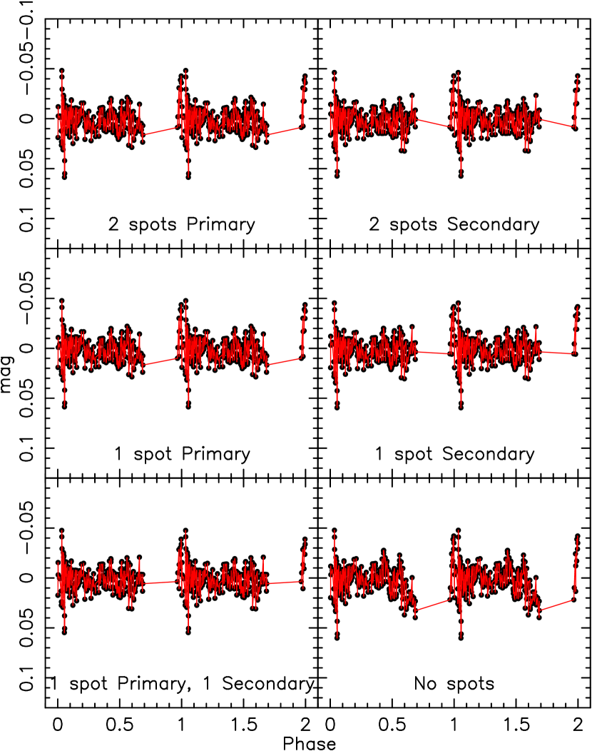
Figure 4: The residuals of the model fits to the $R$-band CCD data for the various spot scenarios: Two spots on the primary star and none on the secondary star (upper left), two spots on the secondary star and none on the primary star (upper right), one spot on the primary and none on the secondary (middle left), one spot on the secondary and none on the primary (middle right), one spot on the primary and one spot on the secondary (lower left), and no spots on either star (lower right).

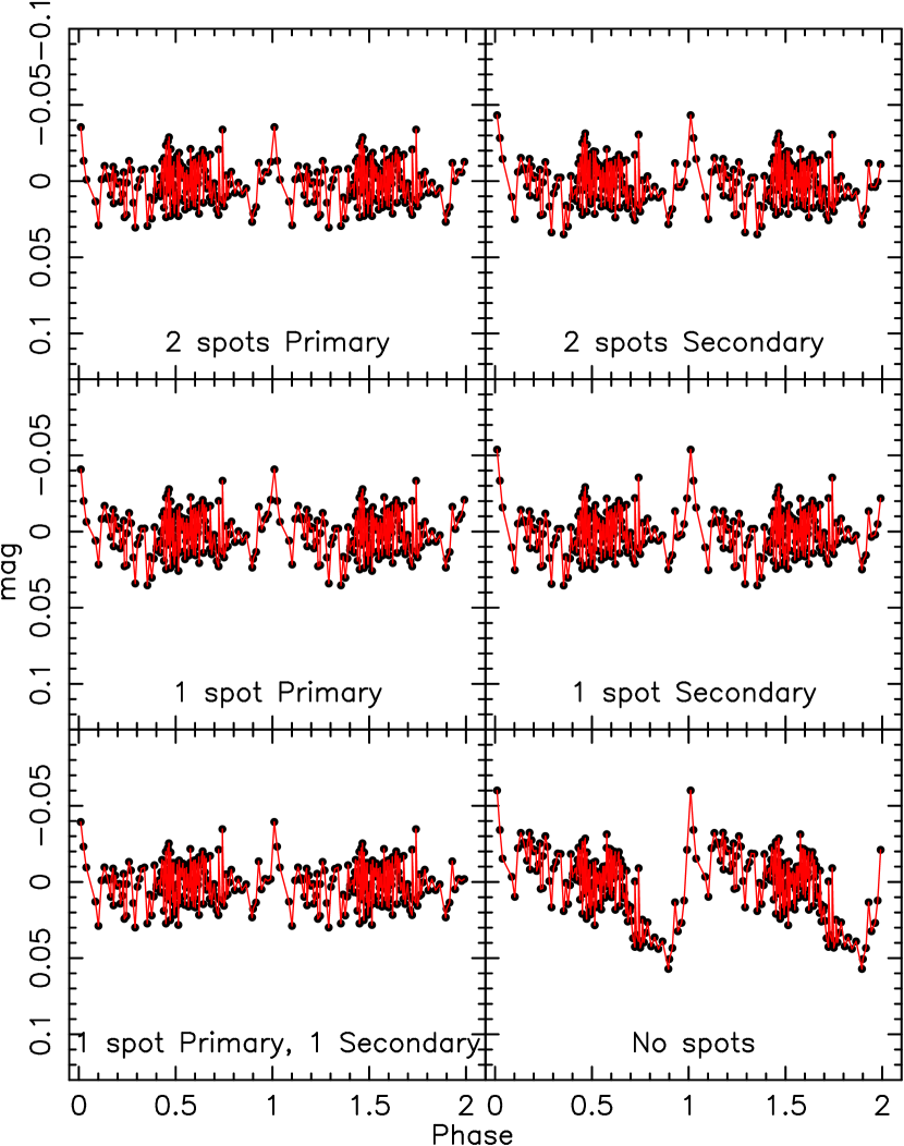
Figure 5: Similar to Figure 4, but for the $R$-band PMT light curve.

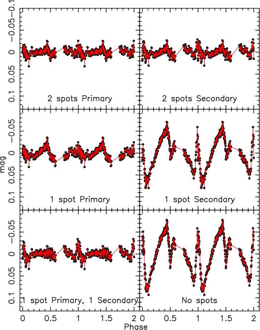
Figure 6: Similar to Figure 4, but for the $R$-band light curve from LR05.

The astrophysical parameters for GU Boo that are currently of most interest to us are the masses and radii of the component stars. In Table 2, we summarize the masses and radii derived from the various data sets (CCD, PMT, and LR05) using the various spot scenarios (no spots, one spot on primary, one spot on secondary, one spot on each, two spots on primary, and two spots on secondary). For each situation, we give the $\chi^{2}$ of the fit (which includes all light curves in the particular data set and both radial velocity curves), the component masses, the component radii, and the differences between our derived values and the values reported in LR05. One can use the $\chi^{2}$ values to determine which spot scenario provides the optimal fit. We find that for the CCD and PMT data, the scenario with one spot on the primary and one spot on the secondary gives the best fit. For the LR05 data, two spots on the primary is optimal. Table 3 gives the input parameters for the best-fitting models for each data set. Also given in Table 3 are the derived rotational velocities of each star. In all cases, the derived values agree with the measured values given in LR05 ($V_{\rm rot}\sin(i)=65$ and $58$ km s^-1 for the primary and secondary, respectively, with no uncertainty given). Figures 1 and 2 show the phased CCD and PMT light curves from Mount Laguna and the best-fitting models. The agreement between the model curves and the observed points is in general very good. Figures 4, 5, and 6 show the $R$-band residuals for the various spot scenarios for the CCD, PMT, and LR05 data, respectively. For the Mount Laguna data, it is hard to tell by eye the differences between the residuals from the various spot scenarios (with the exception of the cases with no spots), in spite of the fact that change in $\chi^{2}$ from the worst case to the best case is significant. On the other hand, the two-spot models are clearly superior to the one-spot models for the LR05 data (Figure 6).

We note some interesting features and trends seen in Table 2 and in Figures 4, 5 and 6. As one might expect, the masses found the fits to the various data sets and the various spot scenarios are very similar since all fits used the same radial velocity curves. A bit more surprising is the fact that the radius of the primary and the radius of the secondary found from the various data sets and spot scenarios generally agree with each other at the $\approx 4\%$ level, although differences of up to about 8% occur for a few of the cases. With one or two exceptions, the radii we found were within $\approx 0.02\,R_{\odot}$ of the values reported in LR05. This is in spite of the fact that the change in $\chi^{2}$ between the worst spot scenario and the best spot scenario for a given data set is large, as noted above. This would seem to suggest that the radii one finds from the light curves is mostly determined by the shapes of the eclipse profiles, and would be within 4 to 5% of the “true” answer in most cases. The spots can further reduce the $\chi^{2}$ of the fit, but seem to add little in terms of the radius determination.

On the other hand, mass and radius determinations at the 2% level or better are needed if one wants to perform detailed comparisons between the measurements and the predicted values from evolutionary models. Thus, for a given data set, one wants to have model light curves that are well matched to the observed light curves. As noted above, for each data set, we found the spot scenario that resulted in the optimal fit. We summarize in Table 4 the masses and radii of the components found from these models. We derived a radius of the primary of $0.6329\pm 0.0026\,R_{\odot}$, $0.6413\pm 0.0049\,R_{\odot}$, and $0.6373\pm 0029\,R_{\odot}$ from the CCD, PMT, and LR05 data, respectively. These values agree with the value reported by LR05 ($R_{1}=0.623\pm 0.016\,R_{\odot}$) at the level of $\approx 2\%$. For the secondary star, we derive radii $0.6074\pm 0.0035\,R_{\odot}$, $0.5944\pm 0.0069\,R_{\odot}$, and $0.5976\pm 0.0059\,R_{\odot}$ from the three respective data sets. The LR05 value is $R_{2}=0.620\pm 0.020\,R_{\odot}$. In this case, our derived radii are all smaller than the LR05 values, with the largest deviation being $\approx 3.5\%$. Although the formal fitting errors are relatively small ($\approx 0.5\%$ for the primary and $\approx 1\%$ for the secondary), it seems that, for a given data set, the accuracy to which we can determine the radii is limited to the $\approx 2-4$% level. Since we don’t know the “true” radii of the stars in the GU Boo binary, it is not immediately obvious if the presence of spots causes us to overestimate slightly the radii or to underestimate slightly the radii. Therefore, taking an average of the three measurements may not bring us closer to the true answer. Extensive Monte Carlo simulations with model binaries might shed some light on this issue.

By now, it is well known that evolutionary models for low mass stars have done a relatively poor job when confronted with mass-radius measurements from eclipsing binaries. In spite of the fact that there may be systematic errors of a few percent on the radius determinations, the measured masses and radii of low mass stars in eclipsing binaries are significantly larger than those predicted based on evolutionary models (e.g., Torres & Ribas 2002; LR05, Bayless & Orosz 2006, Ribas 2006). Recently, there has been speculation that unusually strong stellar activity in these low-mass stars might make them larger than they otherwise would be (Ribas 2006; Torres et al. 2006; López-Morales 2007; Chabrier et al. 2007), and that the changes in the stars caused by stellar activity has not been properly accounted for in the evolutionary models. As discussed here, one or both of the stars in GU Boo have large spots that change with time, and these spots seem to limit our ability to derive radii accurate at the level of $\lesssim 2\%$. Nearly all of the well-studied eclipsing binaries with low-mass stars have orbital periods shorter than $\approx 3$ days. Since the timescale for tidal synchronoziation for these binaries is relatively short (e.g., Zahn 1977), the stars presumably have short rotation periods and higher amounts of activity compared to single stars of similar mass. A recent exception is a binary known as T-Lyr1-17236 (Devor et al. 2008), which has an orbital period of about 8.43 days and components with masses and radii of $M_{1}=0.6795\pm 0.0107\,M_{\odot}$, $M_{2}=0.5226\pm 0.0061\,M_{\odot}$, $R_{1}=0.634\pm 0.043\,R_{\odot}$, and $R_{2}=0.525\pm 0.052\,R_{\odot}$, respectively. Both stars have relatively small rotational velocities, and with such a long orbital period, would still be slowly rotating even if the binary has been circularized because of tidal forces. Devor et al. (2008) show there are no obviously strong indicators of stellar activity in these stars. Although the radius measurements have relatively large uncertainties, Devor et al. (2008) show that both stars have radii consistent with predictions based on evolutionary models.

If the stellar activity is indeed the cause of the disagreement between the measured radii and the radii predicted from evolutionary models, then presumably there is a threshold below which the activity has little or no effect on the overall structure of the star. We have shown (for GU Boo at least) that star spots seem to be a limiting factor in an accurate radius determination, and likewise one would expect that there is also a threshold of spot activity below which the radius determination can become much more precise. A better observational understanding of the former threshold can come from the study of additional long-period binaries. Although these binaries are rare, hopefully more will be discovered in current and future large area surveys (for example the Trans-Atlantic Exoplanet Survey [TrES, Alonso et al. 2004] that led to the discovery of T-Lyr-17236). A better observational understanding of the latter can come from long-term monitoring of the known systems. As we have done for GU Boo, one can observe these binaries at different times and derive radii from independent light curves. The different measurements will have a spread, either large or small, and the size of the spread might be correlated with the level of spot activity.

Table 1: Observations by Dataset, Date, and Band

Data Type	UT date	$N_{B}$	$N_{V}$	$N_{R}$	$N_{I}$
LR05, Kitt Peak	2003-Mar-25	$\cdots$	$\cdots$	$\cdots$	190
	2003-Apr-02	$\cdots$	$\cdots$	$\cdots$	178
	2003-Apr-03	$\cdots$	$\cdots$	107	$\cdots$
	2003-Apr-19	$\cdots$	$\cdots$	163	$\cdots$
	2003-May-02	$\cdots$	$\cdots$	95	254
CCD, Mount Laguna	2005-May-26	$\cdots$	35	36	34
	2005-May-27	$\cdots$	125	121	121
	2005-May-28	$\cdots$	135	139	131
PMT, Mount Laguna	2005-Jun-02	13	13	13	13
	2005-Jun-03	2	2	2	2
	2005-Jun-04	42	42	42	42
	2005-Jun-05	23	23	23	23
	2005-Jun-06	39	39	39	39
	2005-Jun-18	30	30	30	30
	2005-Jun-19	11	11	11	11

Table 2: One and Two Spots Optimization Results

Data Type	Spots	$\chi^{2}$	$M_{1}$	$M_{2}$	$R_{1}$	$R_{2}$	$\Delta M_{1}$	$\Delta M_{2}$	$\Delta R_{1}$	$\Delta R_{2}$
CCD	1 Primary	897.602	0.6111	0.6006	0.6316	0.6224	0.001106	0.001581	0.008593	0.002363
CCD	1 Secondary	893.771	0.6188	0.6058	0.6359	0.6333	0.0088	0.0068	0.0129	0.0133
CCD	2 Primary	890.460	0.6115	0.6006	0.6296	0.6214	0.001505	0.001595	0.006576	0.001406
CCD	2 Secondary	872.868	0.6191	0.6054	0.6473	0.6331	0.0091	0.0064	0.0243	0.0131
CCD	1 Prim  1 Sec	854.273	0.6049	0.5932	0.6329	0.6074	$-0.0051$	$-0.0058$	0.0099	$-0.0126$
CCD	No Spots	995.440	0.6124	0.6027	0.6273	0.6579	0.0024	0.0037	0.0043	0.0379
PMT	1 Primary	1080.768	0.6107	0.5963	0.6429	0.5979	0.000724	$-0.002664$	0.019905	$-0.022113$
PMT	1 Secondary	1088.551	0.6245	0.6105	0.6459	0.6038	0.0145	0.0115	0.0229	$-0.0162$
PMT	2 Primary	1055.538	0.6073	0.5936	0.6413	0.5944	$-0.0027$	$-0.0054$	0.0183	$-0.0256$
PMT	2 Secondary	1053.480	0.6188	0.6059	0.6406	0.6121	0.008756	0.006937	0.017633	$-0.007892$
PMT	1 Prim  1 Sec	1046.102	0.6013	0.5887	0.6195	0.6036	$-0.0087$	$-0.0103$	$-0.0035$	$-0.0164$
PMT	No Spots	1548.052	0.6118	0.6026	0.6226	0.5928	0.0018	0.0036	$-0.0004$	$-0.0272$
Other Data
LR05	1 Primary	1346.136	0.5983	0.5797	0.6286	0.6107	$-0.0117$	$-0.0193$	0.0056	$-0.0093$
LR05	1 Secondary	1657.060	0.6223	0.6033	0.6644	0.6430	0.0123	0.0043	0.0414	0.0230
LR05	2 Primary	1052.124	0.6002	0.5847	0.6373	0.5976	$-0.0098$	$-0.0143$	0.0143	$-0.0224$
LR05	2 Secondary	1134.496	0.6301	0.6126	0.6292	0.6284	0.0201	0.0136	0.0062	0.0084
LR05	1 Prim  1 Sec	1115.721	0.6268	0.6053	0.6448	0.6031	0.0168	0.0063	0.0218	$-0.0169$
LR05	No Spots	8814.927	0.6098	0.6068	0.6055	0.6728	$-0.0002$	0.0078	$-0.0175$	0.0528

Table 3: All Fitted Parameters of the Best Solutions

Data Type:	CCD, Spots: 1 Prim’ 1 Sec’		PMT, Spots: 1 Prim’ 1 Sec’		LR05, Spots: 2 Primary
Parameter	Value	Uncertainty	Value	Uncertainty	Value	Uncertainty	Unit
$\chi^{2}$	854.2734	$\cdots$	1046.1019	$\cdots$	1052.1241	$\cdots$
$M_{1}$	0.6049	$\pm 0.00489$	0.6014	$\pm 0.0106$	0.6002	$\pm 0.0060$	$M_{\odot}$
$R_{1}$	0.6329	$\pm 0.00261$	0.6195	$\pm 0.0077$	0.6373	$\pm 0.0029$	$R_{\odot}$
$\frac{R_{1}}{R_{2}}$	1.0419	$\pm 0.007663$	1.0264	$\pm 0.0161$	1.0666	$\pm 0.0153$
$i$	88.2804	$\pm 0.1433$	88.0500	$\pm 0.2533$	88.6340	$\pm 0.1749$	deg
$K_{1}$	142.0709	$\pm 0.7019$	141.6102	$\pm 0.7922$	141.1003	$\pm 1.1165$	$\rm{km~{}sec^{-1}}$
$T_{1}$	3737.7100	$\pm 12.24$	3701.1500	$\pm 29.4800$	3788.5100	$\pm 6.99$	$\rm{{}^{\circ}K}$
$T_{2}$	3625.8300	$\pm 14.37$	3625.5500	$\pm 31.2600$	3706.3400	$\pm 9.9$	$\rm{{}^{\circ}K}$
$P$	0.48873066	$\pm 1.5\times 10^{-7}$	0.488730245	$\pm 2.9\times 10^{-7}$	0.488718	$\pm 2.165\times 10^{-5}$	day
$T_{0}$	2723.9811	$\pm 0.0002108$	2723.9816	$\pm 0.000492$	2723.9856	$\pm 0.00535$	HJD
$b1$	0.8052	$\pm 0.0286$	0.9476	$\pm 0.0196$	0.9256	$\pm 0.0062$
$b2$	10.7800	$\pm 0.4$	33.7500	$\pm 4.23$	46.4600	$\pm 2.4900$	deg
$b3$	59.0700	$\pm 1.38$	57.8000	$\pm 2.6900$	353.1000	$\pm 1.0100$	deg
$b4$	56.7140	$\pm 0.522$	57.9220	$\pm 5.5700$	38.2680	$\pm 2.0810$	deg
$c1$	0.7539	$\pm 0.0567$	0.5543	$\pm 0.1534$	1.1673	$\pm 0.0192$
$c2$	42.5800	$\pm 2.91$	22.7700	$\pm 3.0100$	104.9300	$\pm 26.9000$	deg
$c3$	54.4400	$\pm 3.16$	48.2200	$\pm 3.6800$	207.5500	$\pm 2.8600$	deg
$c4$	18.0550	$\pm 1.806$	28.8490	$\pm 4.2680$	9.8230	$\pm 0.7860$	deg
$V\sin(i)_{1}$	65.5090	$\pm 0.2670$	64.1180	$\pm 0.7910$	65.9850	$\pm 0.3050$	$\rm{km~{}sec^{-1}}$
$V\sin(i)_{2}$	65.8790	$\pm 0.3570$	62.4730	$\pm 1.3100$	61.8700	$\pm 0.606$	$\rm{km~{}sec^{-1}}$

Table 4: Masses and Radii from All Best Solutions

Data Type	$R_{1}$	$R_{2}$	$M_{1}$	$M_{2}$
CCD (spots: 1 Primary 1 Secondary)	$0.6329\pm 0.0026$	$0.6074\pm 0.0035$	$0.6049\pm 0.0049$	$0.5932\pm 0.0062$
PMT (spots: 1 Primary 1 Secondary)	$0.6413\pm 0.0049$	$0.5944\pm 0.0068$	$0.6073\pm 0.0063$	$0.5936\pm 0.0033$
LR05 (spots: 2 Primary)	$0.6373\pm 0.0029$	$0.5976\pm 0.0059$	$0.6002\pm 0.0060$	$0.5847\pm 0.0090$
Average	0.6372 $\pm 0.0042$	0.5998 $\pm 0.0068$	0.6041 $\pm 0.0036$	0.5905 $\pm 0.0050$
LR05 own fit (spots: 1 Primary 1 Secondary)	$0.6230\pm 0.0160$	$0.6200\pm 0.0200$	$0.6100\pm 0.0070$	$0.5990\pm 0.0060$

References

- Alonso et al. (2004) Alonso, R., et al. 2004, ApJ, 613, L153
- Bayless & Orosz (2006) Bayless, A. J., & Orosz, J., 2006, ApJ, 651, 1120-1155
- Bessell (1990) Besell, M. S., 1990, PASP, 102, 1181
- Çakirli et al. (2009) Çakirli, Ö., İbanoǧlu, C., & Güngör, C. 2009, NewA, 14, 496
- Chabrier et al. (2007) Chabrier, G. Gallardo, J., & Baraffe, I. 2007, A&A, 472, L17
- Creevey et al. (2005) Creevey, O. L., Benedict, G. F., Brown, T. M., Alonso, R., Cargile, P., Mandushev, G., Charbonneau, D., McArthur, B. E., Cochran, W., O’Donovan, F. T., Jiménez-Reyes, S. J., Belmonte, J. A., & Kolinski, D., 2005, ApJ, 625, L127-130
- Devor et al. (2008) Devor, J., Charbonneau. D., Torres, G., Blake, C. H., White, R. J., Rabus, M., O’Donovan, F. T., Mandushev, G., Bakos, G. À., Fürèsz, G., & Szentgyorgyi, A. 2008, ApJ, 687, 1253
- Guenther et al. (1992) Guenther, D. B., Demarque, P., Kim, Y.-C., & Pinsonneault, M. H. 1992, “Standard Solar Model,”, ApJ, 387, 372-393
- Irwin et al. (2009) Irwin, J., Charbonneau, D., Berta, Z. K., Quinn, S. N., Latham, D. W., Torres, G., Blake, C. H., Burke, C. J., Esquerdo, G. A., Fürèsz, G., Mink, D., J., Nutzman, P., Szentgyorgyi, A. H., Calkins, M. L., Falco, E. E., Bloom, J. S., & Starr, D. L. 2009, ApJ, 701, 1436
- López-Morales & Ribas (2005) López-Morales, M., & Ribas, I., 2005, ApJ, 631, 1120-1133
- López-Morales (2007) López-Morales, M. 2007, ApJ, 660, 732
- Orosz & Hauschildt (2000) Orosz, J. A, & Hauschildt, P. H. 2000 A&A, 364, 265-281
- Orosz et al. (2002) Orosz, J.a., Groot, P. J., van der Klis, M., McClintock, J. E., Garcia, M.R., Zhao, P., Jain, R. K., Bailyn, C. D., & Remillard, R. A. 2002a, ApJ, 568, 845-861
- Pols et al. (1997) Pols, O. R., tout, C. A., Schröder, K.-P., Eggleton, P. P., & Manners, J., 1997, MNRAS, 289, 869-881
- Press et al. (1992) Press, W. H., Teukolsky, S. A., Vetterling, W. T., & Flannery, B. P. 1992, Numerical recipes in FORTRAN. The art of scientific computing, 2nd ed. (Cambridge: University Press)
- Ribas (2006) Ribas, I. 2006, Ap&SS, 304 89
- Schröder et al. (1997) Schröder, K.-P., Pols, O. R., & Eggleton, P. P., 1997, MNRAS285, 696-710
- Schuh (2003) Schuh, S. L., Handler, G., Drechsel, H., Hauschildt, P., Dreizler, S., Medupe, R., Karl, C., Napiwotzki, R., Kim, S.-L., Park, B.-G., Wood, M. A., Paparó, M., Szeidl, B., Virághalmy, G., Zsuffa, D., Hashimoto, O., Kinugasa, K., Taguchi, H., Kambe, E., Leibowitz, E., Ibbetson, P., Lipkin, Y., Nagel, T., Göhler, E., & Pretorius, M. L., 2003, A&A, 410, 649
- Stetson (1987) Stetson P. B., 1987, PASP, 99, 191
- Stetson (1990) Stetson, P. B., 1990, PASP, 102, 932
- Stetson (1992a) Stetson, P. B., 1992a, Astronomical Data Analysis Software and Systems I, D. M. Worrall, Biemesderfer, J: Barnes (San Francisco: ASP), 297
- Torres & Ribas (2002) Torres, G., & Ribas, I., 2002, ApJ, 567, 1140-1165
- Torres et al. (2006) Torres, G., Lacy, C. H., Marschall, L. A., Sheets, H. A., & Mader, J. A. 2006, ApJ, 640, 1018
- Wilson & Devinney (1971) Wilson, R. E., & Devinney, E. J., 1971, ApJ, 166, 619
- Zahn (1977) Zahn, J.-P. 1977, A&A, 57, 383