PINGS: the PPAK IFS Nearby Galaxies Survey

Abstract

We present the PPAK Integral Field Spectroscopy (IFS) Nearby Galaxies Survey: PINGS, a 2-dimensional spectroscopic mosaicking of 17 nearby disk galaxies in the optical wavelength range. This project represents the first attempt to obtain continuous coverage spectra of the whole surface of a galaxy in the nearby universe. The final data set comprises more than 50000 individual spectra, covering in total an observed area of nearly 80 arcmin². The observations will be supplemented with broad band and narrow band imaging for those objects without public available images in order to maximise the scientific and archival value of the data set. In this paper we describe the main astrophysical issues to be addressed by the PINGS project, we present the galaxy sample and explain the observing strategy, the data reduction process and all uncertainties involved. Additionally, we give some scientific highlights extracted from the first analysis of the PINGS sample. A companion paper will report on the first results obtained for NGC 628: the largest IFS survey on a single galaxy.

1 Introduction

Hitherto, most spectroscopic studies in nearby galaxies have focused on the derivation of physical and chemical properties of spatially-resolved bright individual H II regions. Most of these measurements were made with single-aperture or long-slit spectrographs, resulting in samples of typically a few H II regions per galaxy or single spectra of large samples like the Sloan Digital Sky Survey (SDSS, York et al., 2000) or other large surveys. The advent of multi-object and integral field spectrometers with large fields of view now offers us the opportunity to undertake a new generation of emission-line surveys, based on samples of scores to hundreds of individual H II regions within a single galaxy and full 2-dimensional (2D) coverage of the disks.

In this paper, we describe the PPAK IFS Nearby Galaxies Survey: PINGS, a project designed to construct 2D spectroscopic mosaics of a representative sample of nearby spiral galaxies, using the unique instrumental capabilities of the Postdam Multi Aperture Spectrograph, PMAS (Roth et al., 2005) in the PPAK mode (Verheijen et al., 2004; Kelz et al., 2006; Kelz & Roth, 2006) at the Centro Astronómico Hispano Alemán (CAHA) at Calar Alto, Spain. “The PMAS fibre PAcK (PPAK) is currently one of the world’s widest integral field units with a field-of-view (FOV) of 74 $\times$ 65 arcsec that provides a semi-contiguous regular sampling of extended astronomical objects” (Kelz, http://tinyurl.com/ppak-aip). This project represents one of the first attempts to obtain 2D spectra of the whole surface of a galaxy in the nearby universe. The observations consist of integral field unit (IFU) spectroscopic mosaics for 17 nearby galaxies ($D\,<\,100$ Mpc) with a projected optical angular size of less than 10 arcmin. The spectroscopic mosaicking comprises more than 50000 spectra in the optical wavelength range. The data set will be supplemented with broad band and narrow band imaging for those objects without publicly available images.

The primary scientific objectives of PINGS are to use the 2D IFS observations to study the small and intermediate scale variation in the line emission and stellar continuum by means of pixel-resolved maps across the disks of nearby galaxies. These spectral maps will allow us to test, confirm, and extend the previous body of results from small-sample studies, while at the same time open up a new frontier of studying the two-dimensional metallicity structure of disks and the intrinsic dispersion in metallicity. Furthermore, the large body of data arising from these studies will also allow us to test and strengthen the diagnostic methods that are used to measure H II region abundances in galaxies.

Previous works have used multi-object instruments to obtain simultaneous spectra of H II regions in a disk galaxy (e.g. Roy & Walsh, 1988; Kennicutt & Garnett, 1996; Moustakas & Kennicutt, 2006a), or narrow-band imaging of specific fields to obtain information of star forming regions and the ionized gas (e.g. Scowen et al., 1996). One important attempt is represented by the SAURON project (Bacon et al., 2001), which is based on a panoramic lenslet array spectrograph with a relatively large FOV of 33 $\times$ 41 arcsec². SAURON was specifically designed to study the kinematics and stellar populations of a sample of nearby elliptical and lenticular galaxies. The application of SAURON to spiral galaxies was restricted to the study of spiral bulges. A recent effort by Rosolowsky & Simon (2008) plans to obtain spectroscopy for $\sim$ 1000 H II regions through the M 33 Metallicity Project, using multi-slit observations. On the other hand, Blanc et al. (2009) obtained IFS observations of the central region of M 51 ($\sim$ 1.7 arcmin²), using the VIRUS-P instrument. However, in spite of the obvious advantages of the IFS technique in tackling known scientific problems and in opening up new lines of research, 2D spectroscopy is a method that has been used relatively infrequently to study large angular-size nearby objects. Recently, PPAK was used successfully to map the Orion nebula, obtaining the chemical composition through strong line ratios (Sánchez et al., 2007b). Likewise, PMAS in the lens-array configuration was used to map the spatial distribution of the physical properties of the dwarf H II galaxy II Zw 70 (Kehrig et al., 2008), although covering just a small FOV ($\sim$ 32 arcsec).

Despite these previous efforts toward IFS of nearby galaxies, the application to obtain complete 2D information in galaxies is a novel technique. Reasons for the lack of studies in this area include small wavelength coverage, fibre-optic calibration problems, but mainly the limited FOV of the instruments available worldwide. Most of these IFUs have a FOV of the order of arcsec, preventing a good coverage of the target galaxies on the sky in a reasonable time, even with a mosaicking technique. Furthermore, in some cases the spectral coverage is not appropriate to measure important diagnostic emission-lines used in chemical abundance studies. Moreover, the complex data reduction and visualisation imposes a further obstacle to more ambitious projects based on 2D spectroscopy. To our knowledge there has been no attempt to obtain point-by-point spectra over a large wavelength range of the whole surface of a galaxy covering all H II regions within it. Similarly to SAURON for early-type galaxies, PINGS will provide the most detailed knowledge of star formation and gas chemistry across a late-type galaxy. This information is also relevant for interpreting the integrated colours and spectra of high redshift sources. In that respect, PINGS represents a leap in the study of the chemical abundances and the global properties of galaxies.

The objectives of this paper are: 1) to provide the background information of the PINGS survey; including a detailed description of the observations, all the data reduction techniques implemented (some of them novel in the treatment of IFS data), and all the uncertainties involved in this process; 2) to offer a general description of the procedures involved in IFS observations of this kind; and 3) to present the PINGS data products and the archival value of this survey. The paper is organised as follows. In § 2 we describe the core scientific objectives of the PINGS project and we discuss some of the many applications of the data set. In § 3 we describe the properties of the galaxy sample selected, while in § 4 we explain the observational strategy and the PINGS observations themselves. In § 5 we present the description of the complex data reduction involved in this IFS survey, while in § 6 we describe the sources and magnitudes of the errors and uncertainties in the data sample. In § 7, we summarise the basic properties of the data, showing a few science case examples extracted from the data set, including the integrated properties, emission line maps and a comparison of line intensity ratios with previously published studies for some galaxies. Finally, in § 8 we give a summary of the article.

2 Scientific Objectives

The study of chemical abundances in galaxies has been significantly benefited from the vast amount of data collected in recent years, either at the neighborhood of the Sun, or at high redshifts, especially on large scale surveys such as the SDSS or the 2dF galaxy redshift survey (Colless et al., 2001). Most studies derived from these observations have focused on linking the properties of high redshift galaxies with nearby objects, as an attempt to understand the principles of the formation and chemical evolution of the galaxies (e.g. see Pettini, 2006). Historically, the metal content of low redshift galaxies has been determined through the nebular emission of individual H II regions at discrete spatial positions, these measurements provide hints on the chemical evolution, stellar nucleosynthesis and star formation histories of spiral galaxies. The chemical evolution is dictated by a complex array of parameters, including the local initial composition, the distribution of molecular and neutral gas, star formation history (SFH), gas infall and outflows, radial transport and mixing of gas within disks, stellar yields, and the initial mass function (IMF). Although it is difficult to disentangle the effects of the various contributors, measurements of current elemental abundances constrain the possible evolutionary histories of the existing stars and galaxies, and thus the importance of the accurate determination of the chemical composition among different galaxy types.

Different studies have shown a complex link between the chemical abundances of galaxies and their physical properties. Such studies are only able to accurately measure the first two moments of the abundance distribution –the mean metal abundances of disks and their radial gradients– and on characterising the relations between these abundance properties and the physical properties of the parent galaxies, for example galactic luminosity, stellar and dynamical mass, circular velocity, surface brightness, colors, mass-to-light ratios, Hubble type, gas fraction of the disk, etc. These studies have revealed a number of important scaling laws and systematic patterns including luminosity-metallicity, mass-metallicity, and surface brightness vs. metallicity relations (e.g. Skillman et al., 1989; Vila-Costas & Edmunds, 1992; Zaritsky et al., 1994; Tremonti et al., 2004), effective yield vs. luminosity and circular velocity relations (e.g. Garnett, 2002), abundance gradients and the effective radius of disks (e.g. Diaz, 1989), and systematic differences in the gas-phase abundance gradients between normal and barred spirals (e.g. Zaritsky et al., 1994; Martin & Roy, 1994). However, these studies have been limited by the number of objects sampled, the number of H II regions observed and the coverage of these regions within the galaxy surface.

In order to obtain a deeper insight of the mechanisms that rule the chemical evolution of galaxies, we require the combination of high quality multi-wavelength data and wide field optical spectroscopy in order to increase significantly the number of H II regions sampled in any given galaxy. The PINGS project was conceived to tackle the problem of the 2-dimensional coverage of the whole galaxy surface. The imaging spectroscopy technique applied in PINGS provides a powerful tool for studying the distribution of physical properties in nearby well-resolved galaxies. PINGS was specially designed to obtain complete maps of the emission-line abundances, stellar populations, and reddening using an IFS mosaicking imaging, which takes advantage of what is currently one of the world’s widest FOV IFU. With this novel spectroscopic technique, the data can be used to derive: 1) oxygen abundance distributions based on a suite of strong-line diagnostics incorporating absorption-corrected H$\alpha$, H$\beta$, [O II], [O III], [N II], and [S II] line ratios; 2) local nebular reddening estimates based on the Balmer decrement; 3) measurements of ionization structure in H II regions and diffuse ionized gas using the well-known and most updated forbidden-line diagnostics in the oxygen and nitrogen lines; 4) rough fits to the stellar age mix from the stellar spectra.

The resulting spectral maps and ancillary data will be used to address a number of important astrophysical issues regarding both the gas-phase and the stellar populations in galaxies. For example, one application will be able to test whether the metal abundance distributions in disks are axisymmetric. This is usually taken for granted in chemical evolution models, but one might expect strong deviations from symmetry in strongly lopsided, interacting, or barred galaxies, which are subject to large scale gas flows. Another important goal is to place strong limits on the dispersion in metal abundance locally in disks; there is evidence for a large dispersion in some objects such as NGC 925 or M 33 (Rosolowsky & Simon, 2008), but it is not clear from those data whether the dispersion is due to non-axisymmetric abundance variations, systematic errors in the abundance measurements, or a real local dispersion. Yet another by product of our analysis will be point by point reddening maps of the galaxies, which can be combined with UV, H$\alpha$, and infrared maps to derive robust, extinction-corrected maps of the SFR.

PINGS can also provide a very detailed knowledge of the role played by star formation in the cosmic life of galaxies. All the important scaling laws previously mentioned tell us that, once born, stars change the ionization state, the kinematics and chemistry of the interstellar medium and, thus, change the initial conditions of the next episode of star formation. Substantially, star formation is a loop mechanism which drives the luminosity, mass and chemical evolution of each galaxy (leaving aside external agents like interactions and mergers). The details of such a complex mechanism are still not well established observationally and not well developed theoretically, and limit our understanding of galaxy evolution from the early universe to present day. In combination with ancillary data, the flux maps computed from the PINGS data will be used to study both the most recent star formation activity of the targets and the older stellar populations. We will be able to identify the gas and stellar features responsible for the observed spectra, to derive the dependence of the local star formation rate on the local surface brightness, a key recipe for modelling galaxy evolution and the environmental dependence of star formation. These data will also provide an important check for interpreting the integrated broad-band colours and spectra of high redshift sources.

Figure 1: Digital Sky Survey images for a selection of objects included in the PINGS sample. On each image, an array of hexagonal fields corresponding to the PPAK aperture is superimposed on scale, showing the IFU mosaicking technique and the observed positions. All images are 10’ $\times$ 10’ and displayed in top-north, left-east configuration.

3 Sample description

In order to achieve the scientific goals described above, we incorporated a diverse population of galaxies, adopting a physically based approach to defining the PINGS sample. We decided to observe a set of local spiral galaxies which were representative of different galaxy types. However, the size and precise nature of the sample were heavily influenced by a set of technical considerations, the principal limiting factor being the FOV of the PPAK unit. We wanted to observe relatively nearby galaxies to maximise the physical linear resolution using the mosaicking technique. However, we also had to take into account the limitations imposed by the amount of non-secure observing time and meteorological conditions for the granted runs. Therefore, the sample size was dictated by a balance between achieving a representative range of galaxies properties and practical limitations in observing time.

When constructing the sample, we also took into account a range of other galaxy properties, such as inclination (with preference to face-on galaxies), surface brightness, bar structure, spiral arm structure, and environment (i.e. isolated, interacting and clustered). We favoured galaxies with high surface brightness and active star formation so that we could have a good distribution of H II regions across the galaxies surface. Galaxies with bars and/or non-typical spiral morphology were also preferred. The final selection of galaxies also took into account practical factors such as optimal equatorial right ascension and declination for the location of Calar Alto observatory, and the observable time per night for a given object above a certain airmass (due to problems of differential atmospheric refraction).

The PINGS sample consists of 17 galaxies within a maximum distance of 100 Mpc; the average distance of the sample is 28 Mpc (for $H_{0}$ = 73 km s^-1 Mpc^-1). The final sample includes normal, lopsided, interacting and barred spirals with a good range of galactic properties and SF environments with multi-wavelength public data. A good fraction of the sample belongs to the Spitzer Infrared Nearby Galaxies Survey (SINGS, Kennicutt et al., 2003), which ensures a rich set of ancillary observations in the UV, infrared, H I and radio.

The sample objects were given a different observing priority based on the angular size of the objects, the number of PPAK adjacent pointings necessary to complete the mosaic, and the scientific relevance of the galaxy. section 3 gives a complete listing of the PINGS sample with some of their relevant properties. The first priority was assigned to medium-size targets such as NGC 1058, NGC 1637, NGC 3310, NGC 4625 and NGC 5474 which are bright, face-on spirals of very different morphological type, with many sources of ancillary data and could be covered with relatively few IFU pointings. The second priority was given to smaller galaxies which fit perfectly in terms of size and acquisition time for the periods during the night when the first priority objects were not observable (due to a high airmass or bad weather conditions) and/or in the case their mosaicking was completed.

NGC 628 (Messier 74) is a special object among the selected galaxies and the most interesting one of the sample. NGC 628 is a close, bright, grand-design spiral galaxy which has been extensively studied. With a projected optical size of 10.5 $\times$ 9.5 arcmin, it is the most extended object of the sample. Although it could be considered too large to be fully observed in a realistic time, we attempted the observation of this galaxy considering that the spectroscopic mosaicking of NGC 628 represents the real 2-dimensional scientific spirit of the PINGS project (see Sánchez et al. 2009, hereafter Paper II). Such a large galaxy would offer us the possibility to assess the body of results from the rest of the small galaxies in the sample and would allow us to study the 2D metallicity structure of the disk and second order properties of the abundance distribution. The observations of this galaxy spanned a period of three-years. Hitherto, NGC 628 represents the largest area ever covered by an IFU, as described briefly in the next section and in detail in Paper II. A special priority was also given to NGC 3184, galaxy which falls between the medium first-priority and large size galaxies. The observations for this object spanned for 2 years, obtaining an almost complete mosaicking (see Figure 1), making this galaxy the 2nd largest object of the sample.

Figure 1 shows Digital Sky Survey images for a selection of galaxies listed in section 3. The mosaicking of the largest objects in the sample, NGC 628 and NGC 3184, consist of 34 and 16 individual IFU pointings respectively, covering almost completely the spiral arms of these two bright grand-design galaxies. The outlying pointings of NGC 1058 and the mosaicking configurations of NGC 3310, NGC 6643 and NGC 7771 are explained in the next section.

In summary, the PINGS sample was selected in a careful way to find a trade-off between the size of the galaxies, their morphological types, their physical properties and the practical limitations imposed by the instrument and the amount of observing time. The result is a comprehensive sample of galaxies with a good range of galactic properties and available multi-wavelength ancillary data, in order to maximise both the original science goals of the project and the possible archival value of the survey.

Table 1: Galaxy properties of the PINGS sample. Col. (1): Galaxy name. Col. (2): Morphological type from the R3C catalog(de Vaucouleurs et al., 1991). Col. (3): Distances in Mpc, references: NGC 628, Hendry et al. (2005); NGC 1058, Eastman et al. (1996); NGC 1637, Saha et al. (2006); NGC 2976, Karachentsev et al. (2002); NGC 3184, Leonard et al. (2002); NGC 3310, Terry et al. (2002); NGC 5474, Drozdovsky & Karachentsev (2000); NGC 6643, Willick et al. (1997); NGC 4625, NGC 6701, NGC 7771, & Stephan’s Quintet: Galactocentric GSR distances derived from the redshift, assumming a value of $H_{0}$ = 73 km s^-1 Mpc^-1. Col. (4): Projected size, major and minor axes at the $B_{25}$ mag arcsec^-2 from R3C, except NGC 7318 from Jarrett et al. (2003). Col. (5): Absolute $B$-band magnitude calculated from the apparent magnitude listed in the R3C catalog and the adopted distances to the system. Col. (6): Redshift, references: NGC 628, Lu et al. (1993); NGC 4625, Fisher et al. (1995); NGC 6701, Theureau et al. (1998); NGC 7770, Woods et al. (2006); NGC 1637, NGC 3310, Haynes et al. (1998); NGC 2976, NGC 5474, Falco et al. (1999, The Updated Zwicky Catalog); NGC 1058, NGC 3184, NGC 6643, NGC 7771, Springob et al. (2005); NGC 7317, NGC 7318a, NGC 7318b, Hickson et al. (1992); NGC 7319, NGC 7320, Nishiura et al. (2000). Col. (7): Heliocentric velocities calculated from $v=zc$, with no further correction applied. Col. (8): Galaxy inclination angle based on the $B_{25}$ mag arcsec^-2 from R3C. Col. (9): Galaxy position angle, measured positive NE, in the $B_{25}$ mag arcsec^-2 except for NGC 1058, NGC 1637, NGC 7317, NGC 7319, NGC 7770, which are based on the $K_{s}$-band (Jarrett et al., 2003), and NGC 3310, NGC 4625, NGC 5474 based on the $r$-SDSS band. Col. (10): Galaxy location.

		Distance	Projected size			$V_{\odot}$
Object	Type	(Mpc)	(arcmin)	$M_{B}$	$z$	(km s-1)	$i$	P.A.	Constellation
(1)	(2)	(3)	(4)	(5)	(6)	(7)	(8)	(9)	(10)
NGC 628	SA(s)c	9.3	10.5 $\times$ 9.5	$-19.9$	$0.00219$	$657$	24	25	Pisces
NGC 1058	SA(rs)c	10.6	3.0 $\times$ 2.8	$-18.3$	$0.00173$	$519$	21	95	Perseus
NGC 1637	SAB(rs)c	12.0	4.0 $\times$ 3.2	$-18.9$	$0.00239$	$717$	36	33	Eridanus
NGC 2976	SAc pec	3.6	5.9 $\times$ 2.7	$-16.9$	$0.00008$	$24$	63	143	Ursa Major
NGC 3184	SAB(rs)cd	11.1	7.4 $\times$ 6.9	$-19.9$	$0.00194$	$582$	21	135	Ursa Major
NGC 3310	SAB(r)bc	17.5	3.1 $\times$ 2.4	$-20.1$	$0.00331$	$993$	39	163	Ursa Major
NGC 4625	SAB(rs)m	9.0	2.2 $\times$ 1.9	$-16.9$	$0.00203$	$609$	29	30	C. Venatici
NGC 5474	SA(s)cd	6.8	4.8 $\times$ 4.3	$-17.9$	$0.00098$	$294$	27	91	Ursa Major
NGC 6643	SA(rs)c	20.1	3.8 $\times$ 1.9	$-19.8$	$0.00495$	$1485$	60	37	Draco
NGC 6701	SB(s)a	57.2	1.5 $\times$ 1.3	$-20.8$	$0.01323$	$3969$	32	24	Draco
NGC 7770	S0	58.7	0.8 $\times$ 0.7	$-19.4$	$0.01414$	$4242$	27	50	Pegasus
NGC 7771	SB(s)a	60.8	2.5 $\times$ 1.0	$-20.8$	$0.01445$	$4335$	66	68	”
Stephan’s Quintet									Pegasus
NGC 7317	E4	93.3	1.1 $\times$ 1.1	$-20.3$	$0.02201$	$6603$	12	150	”
NGC 7318A	E2 pec	93.7	0.9 $\times$ 0.9	$-20.5$	$0.02211$	$6633$	…	…	”
NGC 7318B	SB(s)bc pec	82.0	1.9 $\times$ 1.2	$-20.6$	$0.01926$	$5778$	…	…	”
NGC 7319	SB(s)bc pec	95.4	1.7 $\times$ 1.3	$-20.8$	$0.02251$	$6753$	41	148	”
NGC 7320	SA(s)d	13.7	2.2 $\times$ 1.1	$-17.5$	$0.00262$	$786$	59	132	”

4 Observations

Observations for the PINGS galaxies were carried out at the 3.5m telescope of the Calar Alto observatory with the Postdam Multi Aperture Spectrograph, PMAS (Roth et al., 2005) in the PPAK mode (Verheijen et al., 2004; Kelz et al., 2006), i.e. “a retrofitted bare fibre bundle IFU which expands the FOV of PMAS to a hexagonal area with a footprint of 74 $\times$ 65 arcsec, with a filling factor of 65% due to gaps in between the fibres”. The PPAK unit features a central hexagonal bundle with 331 densely packed optical fibres to sample an astronomical object at 2.7 arcsec per fibre. The sky background is sampled by 36 additional fibres distributed in 6 mini-IFU bundles of 6 fibres each, in a circular distribution at $\sim$ 90 arcsec of the centre and at the edges of the central hexagon. The sky-fibres are distributed among the science ones in the pseudo-slit, in order to have a good characterisation of the sky. Additionally, 15 fibres can be illuminated directly by internal lamps to calibrate the instrument.

All sample galaxies were observed using the same telescope and instrument set-up. We used the V300 grating, covering a wavelength between 3700 – 7100 Å with a resolution of $\sim$ 10 Å FWHM, corresponding to $\sim$ 600 km s^-1. With this set-up we cover all the optical strong emission lines used in typical abundance diagnostic methods (Sánchez et al., 2007b). For the particular setup used in the PINGS survey there was no need to use a order separating filter. The main reason being that the efficiency of the instrument + telescope system (mostly the grating reflectivity and the fibre transmission), drops dramatically at wavelengths shorter than $\sim$ 3600 Å, where the transmission is 1/40000 of the one at the peak intensity for the V300 grating ($\sim$ 5400 Å) and 1/10000 of the value at redder wavelengths covered by our survey ($\sim$ 6500 Å). At bluer wavelengths the efficiency is even lower. Therefore, the system by itself blocks any possible 2nd order contamination up to $\sim$ 7200 Å, and only at larger wavelengths it is required an order separation filter (Kelz et al., 2006). The exposure times were calculated from previous experience with the instrument in order to obtain spectroscopy with S/N $\geq$ 20 in the continuum and S/N $\geq$ 50 in the H$\alpha$ emission line for the brightest H II regions with the given grating.

Different observing strategies were implemented depending on the size and priority of the targets. For those objects with relatively small angular size, single PPAK pointings would not sample the surface of the galaxy with enough spatial resolution, due to the incomplete filling factor of the fibre bundle. In this case, a dithering procedure was applied (Sánchez et al., 2007a). For each individual position in dithering mode, the first exposure was recorded and then, two consecutive exposures with the same acquisition time were recorded, but with small offsets of $\Delta$(RA, Dec) = (1.56, 0.78) and (1.56, –0.78) arcsec with respect to the first exposure. The advantage of this method is that all gaps of the original exposure are covered, and every single point of the dithered field is spectroscopically sampled within the resolution. The pitfalls are that the exposure time and the amount of data to be processed is triple a normal frame, preventing the possibility of applying this method to large mosaics. We used a mean acquisition time per PPAK field in dithering mode (including set-up + integration time) of 2 $\times$ 600 sec. per dithering position for a total of 60 min. exposure; and 3 $\times$ 600 sec. for non-dithered frames.

The observations extended over a period of three-years with a total of 19 observing nights distributed during different observing runs and seasons. For all the objects in the sample, the first exposure was centered in a given geometrical position which, depending on the morphology or a particular mosaicking pattern, may or may not coincide with the bright bulge of the galaxy. Consecutive pointings followed in general a hexagonal pattern, adjusting the mosaic pointings to the shape of the PPAK science bundle as shown in Figure 1. Due to the shape of the PPAK bundle and by construction of the mosaics, 11 spectra of each pointing corresponding to one edge of the hexagon, overlap with the same number of spectra from the previous pointing. This pattern was selected to maximise the covered area, but to allow enough overlapping to match the different exposures taken under variable atmospheric conditions. Exceptions are NGC 2976, NGC 3310, NGC 6643 and NGC 7770 in which the mosaics were constructed to optimise the galaxy surface coverage as explained below.

NGC 628                                                NGC 1058

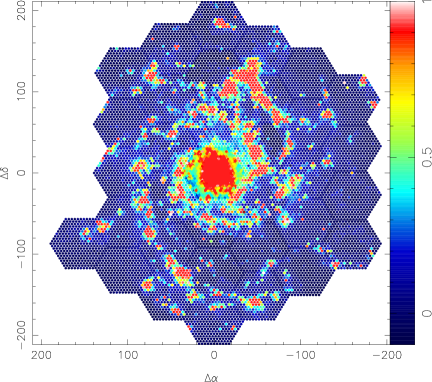
NGC 1637                                                NGC 3184

Figure 2: Examples of the spectroscopic mosaics of NGC 628, NGC 1058, NGC 1637 and NGC 3184. Each panel shows an intensity level narrow-band map centered at H$\alpha$ (6563 Å) in units of 10^-16 erg s^-1 cm^-2 arcsec^-2. Note the effect of surface area coverage for dithered (e.g. NGC 1058, NGC 1637) vs. non-dithered (e.g. NGC 628, NGC 3184) observations, where the gaps between the fibres are clearly seen.

NGC 3310                                                NGC 6701

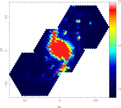
NGC 7770 & 7771                                         Stephan’s Quintet

Figure 3: Spectroscopic mosaics of NGC 3310, NGC 6701, NGC 7770, and the Stephan’s Quintet. Note the effect of dithered (top panels) vs. non-dithered (bottom panels) observations. Units as in Figure 2.

4.1 NGC 628

NGC 628 (or M 74) is an extensively studied isolated grand-design Sc spiral galaxy at a distance of 9.3 Mpc in the constellation of Pisces. The observations for this galaxy totaled six observing nights and 34 different pointings. The central position was observed in dithering mode to gain spatial resolution, while the remaining 33 positions were observed without dithering due to the large size of the mosaic. Seven positions were observed on the 28th October 2006, 19 positions were observed between the 10th and 12th of December 2007, 1 position on August 9th 2008 and the remaining pointings on October 28th 2008. Figure 1 shows the mosaic pattern covering NGC 628 consisting in a central position and consecutive hexagonal concentric rings. The area covered by all the observed positions accounts approximately for 34 arcmin², making this galaxy the largest area ever covered by a IFU mosaicking. The spectroscopic mosaic contains 11094 individual spectra, considering overlapping and repeated exposures (see Paper II, ).

4.2 NGC 1058

NGC 1058 is a well studied Sc spiral with a projected size of 3.0 $\times$ 2.8 arcmin at a distance of 10.6 Mpc, in the constellation of Perseus. The observations for this galaxy were performed on three consecutive nights from the 7th to the 9th December 2007. The mosaic consists of the central position and one concentric ring, covering most of the galaxy surface within one optical radius (defined by the $B$-band 25th magnitude isophote). Ferguson et al. (1998) found the existence of H II regions out to and beyond two optical radii in this galaxy. We tried to observe these intrinsically interesting objects by performing a couple of offsets of 2 and 2.5 arcmin north-east from the central position. These 2 additional position were merged to the original 7 tiles for a mosaic, covering an area of approximately 8.5 arcmin² (see Figure 1). All positions (with the exception of one blind offset) were observed in dithering mode, accounting for a spectroscopic mosaic containing 7944 individual spectra. At the time of the observations, we were able to observe the recently discovered supernova 2007gr, a SN type Ic located at 24”.8 west and 15”.8 north of the nucleus of NGC 1058 between two foreground stars (see subsection 7.4 and Figure 11).

4.3 NGC 1637

NGC 1637 is a SAB distorted galaxy in Eridanus with a projected size of 4.0 $\times$ 3.2 arcmin, at a distance of 12 Mpc. This galaxy presents a clear asymmetry with a third well-defined arm seen in optical images, an unusually extended H I envelope ($D_{H\,{\footnotesize I}~{}}/D_{25}$ = 3.0), and an optical centre that differs from the kinematic centre by 9 arcsec (Roberts et al., 2001). NGC 1637 was observed during December 8th to 10th 2007. The mosaic was built with a central position and one concentric ring of 6 pointings (see Figure 1), covering most of the galaxy surface within one optical radius. The mosaic covers approximately 7 arcmin². This galaxy has a full spectroscopic mosaic containing 6951 individual spectra.

Table 2: Summary of observations of the PINGS sample. Col. (1): Galaxy name. Col. (2): Number of individual IFU positions observed for each galaxy mosaic. Col. (3): Status of the mosaicking; when a percentage is shown, the number in parentheses represents the total number of pointings necessary to cover the optical surface of the galaxy. Col. (4): Total number of spectra for each mosaic. Col. (5): Comments: a) Largest area ever covered by a IFU mosaicking, with a total of $\sim$ 35 arcmin²; b) An offset position of NGC 1058 was not observed in dithering mode (see Figure 2); c) Galaxy with the second largest area of the sample; d) NGC 7770 within the field; e) NGC 7318A and NGC 7318B are included in one field; ^⋆All pointings observed in dithering mode.

Object	Positions	Mosaic	Spectra	Notes
(1)	(2)	(3)	(4)	(5)
NGC 628	34	92% (37)	$13571$	$a$
NGC 1058	9	complete	$7944$	$\star$,$b$
NGC 1637	7	complete	$6951$	$\star$
NGC 2976	2	22% (9)	$662$
NGC 3184	16	84% (19)	$5296$	$c$
NGC 3310	3	complete	$2979$	$\star$
NGC 4625	1	14% (7)	$993$	$\star$
NGC 5474	6	86% (7)	$5958$	$\star$
NGC 6643	3	complete	$2979$	$\star$
NGC 6701	1	complete	$993$	$\star$
NGC 7771	3	complete	$993$	$d$
Stephan’s Q.	4	complete	$1324$	$e$

4.4 NGC 2976

NGC 2976 is a SAc peculiar spiral galaxy with strong emission line spectra with a projected size of 5.9 $\times$ 2.7 arcmin in Ursa Major, at a distance of 3.6 Mpc, being the closest object of the sample. The observations for NGC 2976 were carried out on October 30th 2008. Given the distorted morphology of the galaxy a more convenient mosaic pattern was designed. Two pointings were observed for this object, corresponding to the central region of NGC 2976. The observations were performed in non-dithering mode. The spectroscopic data for this galaxy consist of 662 individual spectra.

4.5 NGC 3184

NGC 3184, a SAB face-on galaxy located in Ursa Major, has the 2nd largest angular size in the sample. It covers an area of 7.4 $\times$ 6.9 arcmin at a distance of 11 Mpc. NGC 3184 has been classified as one of the metal-richest galaxies ever observed (McCall et al., 1985; van Zee et al., 1998), and which has also harboured recently a supernova explosion (SN 1999gi) (Nakano & Kushida, 1999). Three concentric rings are necessary to cover the entire optical disk. Observations for this galaxy were performed on December 10th 2007, following the standard mosaicking pattern with a central position and one complete ring of 7 IFU pointings. Then, on April 27th and 28th 2009, 9 additional pointings were observed covering partially a second concentric ring as shown in Figure 1. The area covered by all the observed positions is $\sim$ 16 arcmin². The spectroscopic data for this galaxy consists of 5296 individual spectra.

4.6 NGC 3310

NGC 3310 is a very distorted spiral galaxy with strong star formation in the constellation of Ursa Major, at a distance of 17.5 Mpc. It covers an area of 3.1 $\times$ 2.4 arcmin in the optical $B$-band, with a very bright central nucleus, surrounded by a ring of luminous H II regions. Different studies of this galaxy suggest a recent merging episode which triggered the burst of star formation (Kregel & Sancisi, 2001; Wehner et al., 2006, and references atherein). Given its morphology, a tailored mosaic pattern was constructed for this galaxy (see Figure 1). Three pointings cover the surface of NGC 3310 with a central position centered in the galaxy’s nucleus and two offsets of (–35, 35) and (35, –35) arcsec in (RA, Dec) in north-west and south-east directions respectively. The observations were carried out on December 8th 2007, and were performed in dithering mode. This galaxy has a full spectroscopic mosaic, which covers an area of approximately 2.8 arcmin². The spectroscopic data for this galaxy totals 2979 individual spectra.

4.7 NGC 4625

NGC 4625 is a low-luminosity SAB, one-armed Magellanic spiral galaxy thought to be interacting with the also single-armed spiral NGC 4618 in Canes Venatici, at a distance of 9 Mpc. The optical size of this galaxy covers an area of approximately 2.2 $\times$ 1.9 arcmin, however Gil de Paz et al. (2005) discovered an extended UV disk reaching to 4 times its optical radius showing evidence of recent star formation. The observation of this galaxy was performed on December 9th 2007 with one single pointing in dithering mode covering the optical radius of NGC 4625. The spectroscopic data for this object consists of 993 individual spectra.

4.8 NGC 5474

NGC 5474 is a strongly lopsided spiral galaxy covering an area of 4.8 $\times$ 4.3 arcmin in Ursa Major, at a distance of 7 Mpc. We observed this galaxy with a standard mosaic configuration consisting of one central position and one concentric ring. All pointings were observed in dithering mode. Observations were carried out in two different periods; 4 positions were observed during August 9th and 10th 2008, while 2 additional pointings were observed on the 27th April 2009. Given the distorted morphology of this galaxy, the central position of the mosaic does not coincide with the bright bulge; a 30 arcsec offset in declination was performed towards the south, so that the area covered by the IFU mosaicking includes most of the optical disk of the galaxy in a symmetric way. The area covered by all the observed positions is approximately 6 arcmin². The spectroscopic data for this galaxy totals 5958 individual spectra.

4.9 NGC 6643

NGC 6643 is a SAc galaxy in Draco, with a projected size of 3.8 $\times$ 1.9 arcmin in the $B$-band, at a distance of 20 Mpc. A tailored mosaic pattern for this galaxy was constructed in order to cover most of its optical area. Three pointings cover the surface of NGC 6643 with a central position centered on the bulge and two offsets of (37, 34) and (–35, –34) arcsec in (RA,Dec) in north-east and south-west directions respectively (see Figure 1). Observations were performed on June 2nd 2008 for the first 2 positions and on August 10th 2008 for the 3rd position, all of them in dithering mode. At the time of the first observing run, we were able to observe the supernova 2008bo, a SN type Ib located at 31” north and 15” west of the nucleus of NGC 6643. This galaxy has a complete spectroscopic mosaic covering an area of approximately 2.8 arcmin². The data consists of 2979 individual spectra. However, due to a technical problem with the instrument set-up, positions 1 and 2 do not cover the usual wavelength range, but are shifted towards the red by approximately 100 Å.

4.10 NGC 6701

NGC 6701 is a small barred spiral in Draco with an angular size of 1.5 $\times$ 1.3 arcmin, at a distance of 57 Mpc. This galaxy was considered to be an isolated galaxy, but studies of NGC 6701 have discovered morphological and kinematical features that are consequence of an interaction, most probably with a companion at 73 kpc in projected distance (Marquez et al., 1996). The observation of NGC 6701 was carried out on August 9th 2008 with one single pointing in dithering mode covering the optical radius of the galaxy (see Figure 1). The spectroscopic data of this galaxy contains 993 individual spectra.

4.11 NGC 7770 and NGC 7771

The main target for this mosaic was the galaxy NGC 7771, a barred spiral in Pegasus with an optical $B$-band size of 2.5 $\times$ 1.0 arcmin at a distance of 59 Mpc. This galaxy is part of an interactive system containing mainly the face-on spiral NGC 7769 and the faint lenticular NGC 7770 (Nordgren et al., 1997). The central part of NGC 7771 contains a massive circumnuclear starburst which was probably triggered by the interaction with the other members of the group (Smith et al., 1999, and references therein). Due to the projected size of this galaxy, the mosaic pattern was constructed with three IFU positions. The central position of the mosaic has an offset of (–15, –15) arcsec in (RA, Dec) from the geometrical centre of the galaxy (see Figure 1). Two additional positions were observed with offsets of (37, 33) and (–37, –33) arcsec. A second member of the interacting group, NGC 7770, a small S0 galaxy with an optical size 0.8 $\times$ 0.7 arcmin was observed within the field of the mosaic pattern. Observations of all 3 positions were performed on October 30th 2008. The spectroscopic data for this galaxy contains 993 individual spectra.

4.12 Stephan’s Quintet

The Stephan’s Quintet is one of the most famous and well-studied group of galaxies, consisting of NGC 7317, 7318A, 7318B, 7319 and 7320 in Pegasus. The distance to this compact group of galaxies has been in debate due to the presence of the brightest member, NGC 7320, which exhibits a smaller redshift than the others, suggesting that is a foreground object lying along the line of sight of the other four interacting galaxies. Although some controversy prevailed (Balkowski et al., 1974; Kent, 1981), recent observations by HST show that individual stars, clusters, and nebulae are clearly seen in NGC 7320 and not in any of the other galaxies (Gallagher et al., 2001; Appleton et al., 2006, and references therein). Four individual pointings in non-dithering mode were observed on August 10th 2008, three of which were centered at the bright bulges of NGC 7317, 7319 and 7320, while the last pointing was centered in configuration to cover NGC 7318A and NGC 7318B (see Figure 1). The spectroscopic data for all pointings of the Stephan’s Quintet contains 1324 individual spectra.

5 Data reduction

The reduction of IFS observations possesses an intrinsic complexity given the nature of the data and the vast amount of information recorded in a single observation. This complexity is increased if one considers creating an IFU spectroscopic mosaic of a given object for which the observations were performed not only on different nights, but even in different years, with dissimilar atmospheric conditions, and slightly differing instrument configurations.

In this section we give an overview of the IFS data reduction process for all the observations of the PINGS sample. In general, the reduction process for the all pointings follows the standard steps for fibre-based integral field spectroscopy. However, the construction of the mosaics out of the individual pointings requires further and more complicated reduction steps than for a single, standard IFU observation. These extra steps arise due to the special mosaicking pattern for some of the objects, the differences in the atmospheric transparence and extinction, slight geometrical misalignments, sky-level variations, differential atmospheric refraction, etc. A complete explanation of the complex data processing for the creation of the PINGS mosaics sample is beyond the scope of this paper, but the reader will find a detailed description of the IFS data reducing in Sánchez 2006 (hereafter San06) and additional information on the mosaicking technique for the PINGS sample in the description of the PPAK-IFS survey of NGC 628 (Paper II).

Following San06, all the data reduction steps can be summarised as follows: a) Pre-reduction. b) Identification of the location of the spectra on the detector. c) Extraction of each individual spectrum. d) Distortion correction of the extracted spectra. e) Application of wavelength solution. f) Fibre-to-fibre transmission correction. g) Flux calibration. h) Allocation of the spectra to the sky position. i) Cube and/or dithered reconstruction (if any).

The raw data extracted from a PINGS observation consists of a collection of spectra, stored as 2D frames, aligned along the dispersion axis. The pre-reduction of the IFS data consists of all the corrections applied to the CCD that are common to the reduction of any CCD-based data, i.e. bias subtraction, flat fielding (in the case of PINGS, using twilight sky exposures), combinations of different exposures of the same pointing and cosmic ray rejection. The pre-reduction processing was performed using standard IRAF packages for CCD pre-reduction steps while the main reduction was performed using the R3D software for fibre-fed and integral-field spectroscopy data (San06) in combination with the E3D visualization software (Sánchez, 2004).

On a raw data frame, each spectrum is spread over a certain number of pixels along the cross-dispersion axis. The spectra are generally not perfectly aligned along the dispersion axis due to the configuration of the instrument, the optical distortions, the instrument focus and the mechanical flexures. Therefore, in order to find the location of each spectrum at each wavelength along the CCD and to extract its corresponding flux, we made use of continuum illuminated exposures taken at each pointing corresponding to a different orientation of the telescope. Each spectrum was extracted from the science frames by co-adding the flux within an aperture of 5 pixels assuming a cut across the cross-dispersion axis found by iterative Gaussian fits (see subsection 6.5 for a detailed description of this reduction step). Since the misalignments of the fibres with the pseudo-slit also affect the wavelength solution, we require lamp exposures obtained at each observed position to find a wavelength solution for each individual spectrum. Wavelength calibration was performed using HeHgCd+ThAr arc lamps obtained through the instrument calibration fibres. Differences in the fibre-to-fibre transmission throughput were corrected by creating a master fibreflat from twilight skyflat exposures taken in every run.

The reduced IFS data can be stored using different data formats, all of which should allow to store the spectral information in association with the 2D position on the sky. Two data formats are widely used in the IFS community: datacubes (3-dimensional images) and Row-Staked-Spectra (RSS) files. Datacubes are only valid to store reduced data from instruments that sample the sky-plane in a regular-grid or for interpolated data. In this case the data are stored in a 3-dimensional FITS image, with two spatial dimensions and one corresponding to the dispersion axis. RSS format is a 2D FITS image where the X and Y axes contain the spectral and spatial information respectively, regardless of their position in the sky. This format requires an additional file (either a FITS or ASCII table), where the position of the different spatial elements on the sky is stored. RSS is widely used by IFUs with a discontinuous sampling of the sky, as it is the case for PPAK. We chose to store the PINGS data in the RSS format, with corresponding position tables.

Once the spectra are extracted, corrected for distortions, wavelength calibrated, and corrected for differences in transmission fibre-to-fibre, they must be sky-subtracted and flux-calibrated. One of the most difficult steps in the data reduction is the correct subtraction of the night sky emission spectrum. In long-slit spectroscopy the sky is sampled in different regions of the slit and a median sky spectrum is obtained by spectral averaging or interpolation. This is possible due to the size of the long-slit compared with the size of the astronomical objects of interest. However, in IFS the techniques vary depending on the geometry of the observed object and on the variation of the sky level for a given observation. By construction, many of the positions of the PINGS mosaics (specially those in the galaxy centre) would fill the entire FOV of the IFU, and none of the spaxels would be completely free of galaxy “contamination”. In this case, we obtained supplementary sky exposures (immediately after the science frames) applying large offsets from the observed positions and between different exposures, we then used these “sky-frames” to perform a direct sky subtraction of the reduced spectra. On the other hand, if the FOV is not entirely filled by the object, it is possible to select those spaxels (i.e. the sky-fibres in the case of PPAK) with spectra free of contamination from objects, average them and subtract the resulting sky-spectrum from the science spectra. We used this technique for observations in the last ring of a mosaic or at the edges of the optical surface of the galaxies, where the sky-fibres bundles did actually sample the sky emission.

Once the sky emission has been subtracted, we need to flux calibrate the observed frames. Absolute spectrophotometry with fibre-fed spectrographs is rather complex; as in slit-spectroscopy, where slit losses impose severe limitations, IFU spectrographs can suffer important light losses due to the geometry of the fibre-arrays. The flux calibration requires the observation of spectrophotometric standard stars during the night. Given that the PPAK IFU bundle does not cover the entire FOV due to gaps among the fibres, the observation of calibration standard stars is prone to flux losses, especially when the standards are not completely well centered in a single IFU spaxel. However we developed a method which takes into account the flux losses due to the gaps in the fibre-bundle, the pointing misalignments and PSF of the observed standard stars, as well as corrections for minor cross-talk effects, airmass, local optical extinction and additional information provided by broad and narrow-band imaging photometry in order to obtain the most accurate possible spectrophotometric flux-calibration within the limits imposed by the instrumentation.

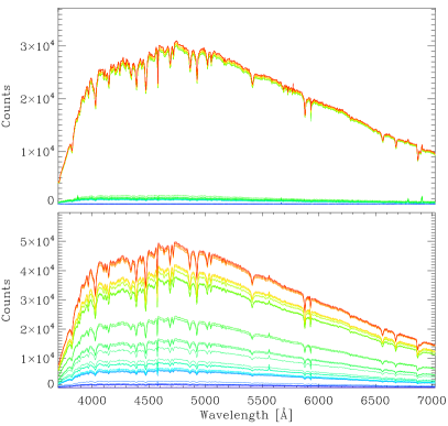
Figure 4: Effect of standard star flux loss due to bad seeing and misalignments. On the top panel, the standard star BD+25d4655 was observed during good atmospheric conditions and was well centred on the central fibre of the PPAK bundle. The figure contains 37 spectra corresponding to the 36 concentric fibres plus the central one. Most of the flux falls in the central fibres (red colour spectra in the online version), while very small residuals are seen in the rest of them (green-blue colour spectra). The bottom panel shows the spectra of the same star observed during turbulent atmospheric conditions and when the star was not well centred in the fibre bundle. In this case the flux is spread over a large number of concentric fibres and the individual contribution of each of them is important for the total observed flux.

A total of six standard stars from the Oke spectrophotometric candles (Oke, 1990) were observed for the purpose of flux calibration during the observing runs. These frames were reduced following the basic procedure described above. To counteract the loss of flux, the observed spectrum of a standard star was obtained by adding up the spectra from consecutive concentric spaxel rings centered on the fibre where most of the standard’s flux is found, until a convergence limit was found (see Figure 4). We then determined a night sensitivity curve as a function of wavelength by comparing the observed flux with the calibrated spectrophotometric standard spectrum considering the filling factor of the fibre-bundle. We applied this function to the science frames considering corrections for the airmass and the optical extinction due to the atmosphere as a function of wavelength to get relative flux-calibrated spectra for each position.

Figure 6 shows the shape and relative magnitude of nine sensitivity curves obtained during the three years of observations. The difference in the vertical scale reflects the variation of the spectrophotometric transmission during different nights and observing runs (the flux calibration obtained by applying these sensitivity curves is just a relative one, an absolute calibration is obtained by re-scaling by a factor derived after the comparison with the broad-band imaging by applying the method described below). However, the differences on the shape from one sensitivity curve to another as a function of wavelength, reflect the intrinsic dispersion of the flux calibration. The bottom panel of Figure 6 shows the variation of the sensitivity curves as a function of wavelength after a grey shift with respect to an arbitrary spline fitting normalised at the wavelength of H$\beta$ (4861 Å). This normalisation wavelength was chosen as most spectroscopic studies normalise the observed emission line intensities to the flux in H$\beta$. The maximum variation from the blue end of the spectrum compared to the red one is of the order of $\sim$ 0.15 mag, corresponding to a maximum calibration error of $\sim$ 15% due solely to the intrinsic dispersion in the relative flux calibration. However, the actual RMS is less than 0.1 mag, corresponding to a typical error in the relative flux calibration of less than 10%.

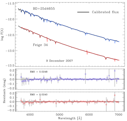
Figure 5: Observed standard stars on the 9th December 2007. The top panel figure shows a comparison of the night flux calibration applied to the observed stars (in colour in the online version) and the corresponding calibrated fluxes. The panel below show the residuals in magnitudes as a function of wavelength for each star. The points with relatively large deviations are due to strong sky emission lines and cosmetic defects of the CCD.

For those galaxies with suitable multi-band photometric data available in the literature (e.g. NGC 628, NGC 3184, NGC 4625, NGC 5474), we used the first-order calibration of either the central pointing of a mosaic or the position with the highest S/N and best sky-subtraction to perform an additional correction to the absolute flux calibration by comparing the convolved spectra observed in this field (taking into account fibre apertures and filters’ response functions) to the corresponding flux measured by $B$, $V$, $R$ broad-band and H$\alpha$ narrow-band imaging photometry for the same position. This procedure ensures a very precise flux calibration and sky extinction correction for this master pointing. To our knowledge, no other IFS observations have ever attempted to get such (instrument-limited) spectrophotometry accuracy. All galaxies belonging to the SINGS sample were corrected by this method using their ancillary data as described in more detail in Paper II.

After reducing each individual pointing with a first-order flux calibration and with the help of the absolute flux-calibrated master pointing, we built a single RSS file for the whole mosaic following an iterative procedure. The process starts in the master pointing chosen for a specific mosaic, i.e. the pointing that has the best possible flux calibration and sky extinction correction, with the best signal-to-noise and the most optimal observing conditions regardless of the geometric position of the pointing in the mosaic. Taking this master pointing as a reference, the mosaic is constructed by adding consecutive pointings following the particular mosaic geometry. During this process, the new added pointing is re-scaled by using the average ratio of the brightest emission lines found in the overlapping spectra (which is then replaced by the average between the previous pointing and the new re-scaled spectra). In most cases the scale factor is found to be between 0.7 and 1.3 with respect to the master pointing.

However, this ratio is wavelength dependent (specially in the cases of variable photometric conditions between the observations). Therefore as a second-order correction, we fitted the variations found between the previous pointing and the new re-scaled overlapping spectra to a low order polynomial function and divided all the spectra in the new pointing by the resulting wavelength dependent scale. This correction has little effect on the data when the observations were performed during the same or consecutive nights, as it is the case for the small mosaics. However, we accounted variations after all the possible corrections of the order of 10-15% in the extreme cases when the observations were carried out at different epochs (e.g. NGC 628, NGC 3184). This level of error is what we expect from observations performed during different nights and observing runs, reflecting the variation of the spectrophotometric transmission from night to night (see Figure 6). The procedure was repeated for each mosaic until the last pointing is included (except for the Stephan’s Quintet, where not actual overlapping occurs), ending with a final set of individual spectra and their corresponding position tables. This process ensures a homogenous flux calibration and sky extinction correction for the entire data set.

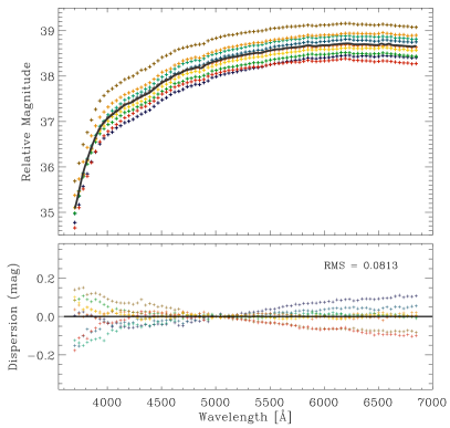
Figure 6: Variation of the spectrophotometric transmission as a function of wavelength. The top panel shows nine sensitivity transmission curves using different calibration standard stars. The thick dark line is a 3rd degree spline fitting to the data. The panel below shows the dispersion in magnitudes after a grey re-scaling of all the sensitivity curves with respect to the spline fit normalised at the H$\beta$ wavelength (4861 Å).

6 Errors and uncertainties in the data sample

During the process of data reduction and basic analysis, we have identified several possible sources of errors and uncertainties in the PINGS data set. Each of them contribute in a different way and magnitude to the overall error budget associated with the observations. These are in order of importance: 1) sky subtraction, 2) flux calibration, 3) differential atmospheric refraction (DAR), 4) cross-talk, and 5) second order spectra. In this section we describe the nature of each of these sources of errors, the tests performed in order to understand their effects on the accuracy of the data, and the techniques applied to minimise them.

6.1 Sky subtraction

As mentioned before, sky subtraction is one of the most difficult steps in the IFS reduction process and it is particularly complex for the nature of the observing technique of PINGS. As described in Sánchez (2006), a deficient sky subtraction in this sort of data has several consequences: “the contamination of the sky emission lines along the spectra which prevents the detection and/or correct measurement of relatively weak nebular emission lines (e.g. the weak temperature sensitive [O III] $\lambda$4363, which is located in the same spectral region as the strong Hg I $\lambda$4358 sky line), and also affects the shape and intensity of the continuum, which is important for the analysis of the stellar populations and the determination of reddening”. In fact, we made use of the mosaicking method in order to find the best possible sky subtraction. Due to the shape of the PPAK bundle and by construction of the mosaics in the standard mosaic configuration, 11 spectra of a given pointing (corresponding to one edge of the hexagon) overlap with the same number of spectra from the previous pointing (see NGC 628 or NGC 3184 in Figure 2). This allows the comparison of the same observed regions at different times and with different atmospheric conditions.

For a non-standard configuration the number of overlapping fibres is larger (e.g. NGC 3310). These overlapping spectra can be compared and used to correct for the sky emission of the adjacent frame. However, prior to performing the sky subtraction it is required to visually check that no residual of the galaxy is kept in the derived spectrum. This can be the case if the transmission changed substantially during the observation of the adjacent frames. These techniques proved to result in good sky subtraction in most cases. On the other hand, when we were forced to obtain supplementary large-angle offset sky-exposures for the inner pointings in the mosaics that were completely filled by the target, we found that when the sky exposure is taken within a few minutes of the science exposure it produces a good subtraction. For those cases in which the atmospheric conditions changed drastically and/or the sky subtraction appeared to be poor, we combined different sky frames with different weights to derive a better result.

One way of assessing the goodness of the sky subtraction is to check for sky residuals in the subtracted spectra. The galaxy mosaic more prone to be affected by residuals in the sky subtraction is NGC 628, which as explained in section 4, was observed during six nights along four observing runs. Therefore we would expect that the spectroscopic mosaic of this galaxy would show the most extreme effects due to the sky subtraction to be found in the PINGS sample, given all the variations in transparency and photometric conditions of the night-sky along the three years of observations.

In order to obtain a quantitative assessment of the quality of the sky subtraction, we performed two different data reductions of the spectroscopic mosaic of NGC 628. In the first reduction, the sky subtraction was performed directly with the average spectrum of the sky fibres at each position, without considering the overlapping spectra between pointings, and not accounting for the object contamination in the sky fibres. Therefore, in this first reduction we applied a “poor” sky subtraction. For the second reduction, we applied an individual sky subtraction per mosaic position using the techniques described above, i.e. applying corrections using the overlapping spectra, checking for galaxy residuals in the derived sky spectrum, using the sky exposures obtained by large offsets for the most internal regions of the galaxy, and combining different sky frames with different weights in those cases when there were important changes in the transmission between pointings observed during the same night. We refer to this reduction as the “refined” sky subtraction.

Airglow is the most important component of the light of the night-sky spectrum at Calar Alto observatory, although a substantial fraction of the spectral features is due to air pollution (Sánchez et al., 2007). The strongest sky line in the Calar Alto night-sky spectrum is the [O I] $\lambda$5577 line, followed by the [O I] $\lambda$6300 line, both produced by airglow with a notorious stronger effect near twilight. A deficient sky subtraction can be recognised by residual features of the sky lines in the derived spectra, this effect is clearly seen in the [O I] $\lambda$5577 sky line which is located in a spectral region without any important nebular emission line. In general terms, (without considering variations in the transparency of the sky), a residual in emission of this line would imply a subtraction of the sky spectrum of slightly lower strength than required, while an absorption feature would imply an over-correction.

In order to make a comparative analysis of the strength of the sky residuals in the two data reductions of NGC 628 described above, we measured the equivalent width (EW) of the residual features centered at the [O I] $\lambda$5577 line. For numerical reasons (regions of null continuum), the local continuum in the neighbourhood of the [O I] $\lambda$5577 sky line was re-scaled to a flux level of 10^-16 erg s^-1 cm^-2 Å^-1 in every single spectrum of both mosaics. EWs with negative sign correspond to residual emission features, while positive EWs correspond to absorption features.

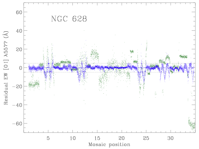
Figure 7: Equivalent width values for the emission and absorption residual features of the [O I] $\lambda$5577 sky line as a function of the observed position for the spectroscopic mosaic of NGC 628. Positive values correspond to absorption features, while negative values to emission residuals. The local continuum level was re-scaled to the same value in order to make this comparison. The green dots (in the online version) correspond to a poor sky subtraction, while the blue dots represent the refined reduction as explained in the text. The two horizontal dotted lines mark the threshold EW values of residuals features corresponding to a good sky subtraction.

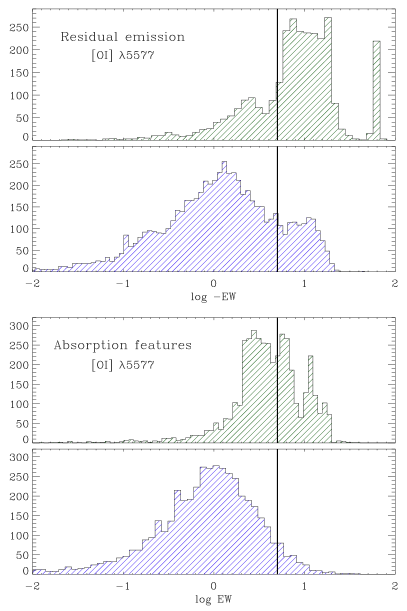
Figure 8: Histograms of the EW residual features shown in Figure 7. The top panels shows the distribution of EW values for the emission residuals. The bottom panels shows the EW values for the absorption features. All EW values are shown in logarithmic scale (assuming a positive EW value for the emission residuals). The top histograms in both cases correspond to the poor sky subtraction, while the bottom histograms correspond to the refined reduction (green and blue colour histograms in the online version). The $\sim$ 5 Å EW threshold value is shown as the vertical line in all the histograms, residual values to the right of this line can be considered a deficient sky subtraction as explained in the text.

Figure 7 shows the value of the EW residuals for the [O I] $\lambda$5577 line for both data reductions as a function of the pointing position in the spectroscopic mosaic. Each position bin contains 331 values corresponding to the number of spectra per pointing, a total of 11104 values are shown, corresponding to the 34 positions observed for NGC 628. The green dots correspond to the poor sky subtraction reduction, while the blue dots correspond to the refined sky subtraction (see the online version of this plot). There is a considerable amount of scatter of the EW residual value for the poor sky subtraction compared to the refined one. In the first two pointings of the mosaic (which correspond to central positions of the galaxy), there are strong residuals in emission for the poor reduction, while the residuals have been minimised in the refined one. Figure 7 shows clear evidence of those pointings in which the sky transparency varied by a considerable amount (positions 4, 5, 11, 12, 23, 24, 28, 29, 33, 34). In all the pointings, the scatter in the residuals is improved in the refined reduction with respect to the first one. This effect is more notorious between positions 13 to 22. The poor sky subtraction yields very strong sky residuals in emission for positions 33 and 34, while in the refined reduction these are minimised.

At the chosen continuum level used for this exercise, a (absolute) value of 5 Å in EW for the [O I] $\lambda$5577 residual line in emission corresponds approximately to a flux intensity value of 5 $\times$ 10^-16 erg s^-1 cm^-2, while a value of 10 Å corresponds to $\sim$ 10 $\times$ 10^-16 erg s^-1 cm^-2. The average flux intensity of the [O I] $\lambda$5577 sky line in Calar Alto is of the order of 33 $\times$ 10^-16 erg s^-1 cm^-2 (Sánchez et al., 2007). However, from a sample of 500 sky spectra acquired during the three years of observation we measured the intensity of the [O I] $\lambda$5577 in the range between 30 and 60 $\times$ 10^-16 erg s^-1 cm^-2, with a mean value of 44. Therefore, a value of 5 Å in EW for a residual emission feature would correspond to $\sim$ 8–10% of the total emission of the [O I] $\lambda$5577 line. Visual inspection of the spectra with emission residual of the order of 5 Å in EW confirms that this value could be considered as the threshold for a good sky subtraction. Spectra with emission or absorption residuals with absolute EW values less than 5 Å could be considered to have a good subtraction, for features above this value the effects of a deficient sky subtraction are evident.

The two horizontal dotted lines in Figure 7 indicate the $\pm$5 EW threshold value for both emission and absorption features. These two lines encompass a region for which the spectra can be considered with a good sky subtraction. The poor sky subtraction (green) shows a lot of scatter and a small fraction of the spectra falls within these limits. On the other hand, for the refined reduction (blue) a total of 9629 spectra fall within these limits, i.e. 87% of the total mosaic. The number of spectra with sky subtraction problems for which $|$EW$|$ $>$ 5 Å is 1475, i.e 13% of the mosaic, these spectra are found in those pointings with extreme transparency variations as expected.

Figure 8 shows the histograms of the EW values for both data reductions, the poor sky subtraction in green and the refined reduction in blue colour following Figure 7 (see the online version of this plot). The top panels show the distribution of residual emission values, while the bottom panels show the absorption residual features for the [O I] $\lambda$5577. The $\sim$ 5 Å EW threshold value is shown as the vertical line in the histograms, residual values to the right of this line can be considered a deficient sky subtraction. Visual inspection of the spectra shows that, at the continuum level used for this comparison, emission or absorption features with values of log($|$EW$|$) $\leq$ 0 could be considered negligible and within the statistical noise of the spectra. The residual emission histograms show that the poor sky subtraction produces a large number of strong residuals with values of $|$EW$|$ $>$ 5 Å, even reaching $|$EW$|$ $\sim$ 60 Å. The majority of the residual values in refined sky subtraction are found at log($|$EW$|$) $\sim$ 0, corresponding to negligible residual values, however there is a small tail of strong emission residuals for which $|$EW$|$ $>$ 5 Å ($\sim$ 18% of the total emission residuals). The distribution of EW values of the absorption features for the poor subtraction is approximately centered at the threshold limit, while for the refined reduction, the values are nearly normally distributed with a centre value of log(EW) $\sim$ 0 with a small tail of strong absorption values ($\sim$ 7%) due most likely to an over subtraction of the sky spectrum.

The refined sky subtraction was the final adopted one for the spectroscopic mosaic of NGC 628. All the sky subtraction techniques implemented showed that the quality of the derived spectra was improved by a considerable amount compared to a standard sky subtraction. Most of the sky residuals are within the limits of a reasonably good sky subtraction. The spectra with strong features are found for those positions in which the photometric conditions changed drastically during the night or observing run. This residual analysis allows to identify those pointings with strong sky variations and thus, to flag the spectral data for future analysis. The sky subtraction for the rest of the PINGS sample was performed similarly to the refined technique described above. Therefore we applied the best possible sky subtraction to all the spectroscopic mosaics within the limitations imposed by the IFS data itself.

6.2 Detection of the [O III] $\lambda$4363 line

The Hg $\lambda$4358 sky line strongly affects any attempt to measure precisely the emission of the faint temperature-sensitive [O III] $\lambda$4363 line in any object with a low redshift. The fact that the strength of this line decreases with increasing abundance (Bresolin, 2006), in combination with typically faint H II regions and low spectroscopic resolution limits importantly the detectability of this key diagnostic line.

In order to assess the significance of the detection of the [O III] $\lambda$4363 given the contamination of the Hg $\lambda$4358 sky line in our data, we performed a simulation of the detectability of the [O III] $\lambda$4363 line for a given range of redshifts and line intensity strengths. We simulated a pure emission line spectrum including the H$\gamma$ $\lambda$4340 and [O III] $\lambda$4363 lines at the same spectral resolution of the PINGS observations; we assumed a normally distributed I($\lambda$4363)/H$\gamma$ ratio with a mean value of 0.10 $\pm$ 0.05, corresponding to typical values found in previous spectroscopic studies where the [O III] $\lambda$4363 line was detected in H II regions within the metallicity range of the PINGS sample (e.g. McCall et al., 1985); we did not consider higher ratios ($\sim$ 0.25 $\pm$ 0.10) which are representative of extremely low metallicity objects (e.g. Pagel et al., 1992; Izotov & Thuan, 2004). We added a random statistical noise of 0.05 RMS at the continuum level constructed from the observed spectroscopic data. A sample of 540 sky spectra were selected among all the observing runs during the three years of observations (considering very different photometric conditions). A flux calibrated sky spectrum was created out of these selected spectra. This sky spectrum was added to the previous emission line plus the noise described above to create a simulated “observed” spectrum. An average sky spectrum constructed from a random subset of 36 sky spectra (the number of PPAK sky-fibres) was then subtracted from the simulated “observed” spectrum to obtain a “sky-free” spectrum.

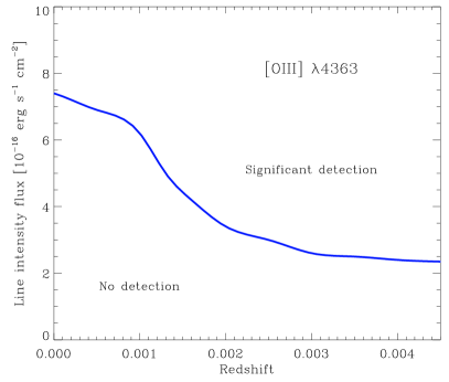
Figure 9: Detectability of the [O III] $\lambda$4363 line as a function of redshift and line strength according to the simulation described in subsection 6.2. For a given redshift, the [O III] $\lambda$4363 can be significantly detected for flux values above the thick line, which marks the region at which the difference between the observed and simulated line intensity is of the order of 15%. The contamination effect of the Hg $\lambda$4358 disappears for redshift values larger than 0.004.

Emission line intensities were then measured simultaneously for both lines in the simulated “sky-free” spectrum using the techniques described in subsection 7.2. These line intensities were then compared with the flux of the pure emission lines. For a given redshift, we varied the emission line strengths of the simulated spectrum from high to lower values until the significance of the detection of the [O III] $\lambda$4363 fell drastically. We performed 500 realisations of the emission line intensity measurements for a given redshift and for a given line strength. Figure 9 shows the results of the simulation, the thick line represents the region at which the difference between the line intensity measured from the simulated “sky-free” spectrum and the flux from the pure emission line is of the order of 15%. According to the simulation, observed flux values of the [O III] $\lambda$4363 above this line can be significantly detected at a given redshift. For flux values below this region the significance of the detection is negligible as it is mostly affected by the statistical noise of the data. The contamination effect of the Hg $\lambda$4358 disappears for redshift values larger than $\sim$ 0.004, where the detectability of the [O III] $\lambda$4363 depends on the signal-to-noise of the spectrum at low line-intensity levels. Experience with the data has proven that the simulation described in this section places very good limits on the detectability and potential measurement of this faint line, although after detection, individual and visual inspection of the spectra has to follow in order to correctly assess the usefulness of this line.

6.3 Flux calibration

Several refinements in the observation technique and standard flux recovery were applied to the pipeline which improved substantially the accuracy of the sensitivity functions obtained after every standard candle observation. During most of the observing runs we observed different standard stars per night at different airmasses in order to asses the variation in transmission and its effect on the relative flux calibration.

We generated several sensitivity curves following the standard pipeline procedure in R3D, changing the key parameters that could affect the accuracy of the derived sensitivity function (e.g. order and type of the fitting function, extinction, airmass, smoothing, etc.). Furthermore, we made a comparison of the response curves obtained through R3D and the ones obtained using standard long-slit flux calibration routines in IRAF after performing all the appropriate corrections and transformations for the two different kinds of data. We even derived whole-run sensitivity curves after the combination of several response curves for a given observing run and applied the derived calibration to the observed standard candles as a proof of self-consistency. In all cases, we found very consistent results in the final relative flux calibration. As described in section 5, even without a re-calibration using broad-band imaging, the spectral shape and features are reproduced within the expected errors for an IFS observation ($\sim$ 20% in the absolute sense) along the whole spectral range, with a small increase in the blue region ($\lambda<$ 3800 Å) due in part to the degradation of the CCD image quality and instrumental low sensitivity towards the blue ($\sim$ 2 – 5%, telescope/atmosphere excluded) in this spectral region .

For those galaxies with available multi-band photometric data, small differences in the transmission curves of the filters and astrometric errors of the built mosaics bring some uncertainties in the derived flux ratios that contribute to the overall standard deviation when applying the photometric re-calibration described before. The errors in the first case are difficult to estimate, however the latter ones were estimated by simulating different mosaic patterns by applying normally distributed random offsets of the simulated fibre-apertures with mean values of 0.3, 0.5 and 1.3 arcsec on the broad-band images and then comparing the extracted spectrophotometry. From the results of these simulations and considering that the IFS mosaics were re-centered using the information directly from the aperture photometry, we expect that the location of the fibres lies within 0.5 arcsec, and therefore the error due to the uncertainty in the astrometry would be of the order of 10%. Based on these results, we estimate a spectrophotometry accuracy better than $\sim$ 0.2 mag, down to a flux limit corresponding to a surface brightness of $\sim$ 22 mag/arcsec² (see Paper II, ) when we apply the re-calibration derived by the flux ratio analysis. In the following section we compare our data with previously published spectrophotometrically calibrated data. The spectral shape, the spectral features and emission line intensities match remarkably well, even for those objects for which no re-calibration was performed (see Figure 11). As stated above, to our knowledge no other IFU observation has ever implemented such corrections in order to obtain an instrumental-limited spectrophotometry accuracy as in this work.

6.4 Differential Atmospheric Refraction

An important systematic effect in any spectroscopic observation is due to the refraction induced by the atmosphere, which tends to alter the apparent position of the sources observed at different wavelengths. By definition, there is no refraction when the telescope is pointed at the zenith, but for larger zenith angles the effect becomes increasingly significant. For IFU observations, this has the consequence that, when comparing for example the intensities at two different wavelengths (e.g the emission line ratio of a source), one will actually compare different regions, given that different wavelengths are shifted relative to each other on the surface of the IFU. In theory, one is capable of performing a correction of DAR for a given pointing without requiring knowledge of the original orientation of the instrument and without the need of a compensator, as explained by Arribas et al. (1999). The correction of DAR is important for the proper combination of different IFS exposures of the same object taken at different altitudes and under different atmospheric conditions, and for the proper alignment of a mosaic and dithered exposures, as it is the case of most PINGS observations. An IFS observation can be understood as a set of narrow-band images with a band-width equal to the spectral resolution (San06). These images can be recentered using the theoretical offsets determined by the DAR formulae (Filippenko, 1982) by tracing the intensity peak of a reference object in the FOV along the spectral range, and recentering it. The application of this method is basically unfeasible in slit spectroscopy, which represents one additional advantage of IFS. The correction can be applied by determining the centroid of a particular object or source in the image slice extracted at each wavelength from an interpolated data cube. Then, it is possible to shift the full data cube to a common reference by resampling and shifting each image slice at each wavelength (using an interpolation scheme), and storing the result in a new data cube. A pitfall of this methodology is that the DAR correction imposes always an interpolation in the spatial direction as described above, a 3-dimensional (3D) data cube has to be created for each observed position, reducing the versatility given by the much simpler and handy RSS files.

We have to note here that the widely accepted formulation summarised by the work of Filippenko and the concept of parallactic angle are just a first order approximation to the problem. All this theoretical body is based on the assumption that all different atmospheric layers have an equal refraction index, are flat-parallel and perpendicular to the zenith. While this approximation is roughly valid, there are appreciable deviations due to the topography and landforms at the location of the telescope, since they alter considerably the structure of the low-altitude atmospheric layers. Therefore, the “a posteriori” correction of the DAR effect, only possible when using IFS, is the most accurate approach to the problem.

In general, the effects due to DAR in IFS are only important for IFUs with small spatial elements ($\leq$ 1.5 arcsec) while for large ones (as it is the case of PPAK), the effect is mostly negligible, as experience with the instruments shows, especially when the airmass of the observations is 1.1 or below (Sandin et al., 2008). According to the DAR formulas one can calculate the angular separation in arcsec due to this effect for two different wavelengths under typical atmospheric conditions for a range of airmasses (Filippenko, 1982, Table 1). If we consider for example the wavelengths of H$\alpha$ at $\lambda$6563 and [O II] $\lambda$3727 emission lines, the angular separation due to DAR is smaller than the radius of the PPAK fibres (1.35 arcsec) for airmasses below 1.3. Nevertheless, for each object in the sample we analysed those pointings which were observed at an airmass $>$ 1.2 in order to test any effects due to DAR in our data. We transformed these individual pointings into 3D data cubes (with a scale of 1”/pixel) and we selected suitable sources within the field (e.g. foreground stars, compact bright emission line regions) to perform a DAR correction creating continuum maps of these bright sources and looking for spatial deviations along the dispersion axis. No significant intensity gradients were found in any of the test fields. Additionally, we looked for regions in which we could observe emission in the blue (e.g. [O II] $\lambda$3727) but no emission in the red (e.g. H$\alpha$ $\lambda$6563) and vice versa. In most of the cases we did not find strange [O II]/H$\alpha$ ratios, although for some pointings we did not have enough bright H II regions to perform this exercise. However, for a number of pointings we did find peculiar deviations from the flux measured in both part of the spectra. All these pointings were observed with an airmass $>$ 1.4 and correspond to: NGC 1637 (all 7 dithered pointings), NGC 6701 (all 3 pointings), and NGC 5474 (pointings 3, 4 & 5). These particular pointings could be individually converted to 3D data cubes and be further analysed and corrected for any DAR effects. In the case of particular studies which require a degree of spatial precision, one has to bear in mind the significance of the spatial-spectral information derived from the individual fibres of these pointings. Integrated spectra over a large aperture ($\sim$ 5 arcsec) could be considered reliable.

Considering in general that the effects of DAR are very small given the relatively large size of the spatial elements of PPAK, that $\sim$ 70% of the observations were performed with an airmass $\leq$ 1.35, and that we found no significant evidence of DAR effects in the analysis of our data (apart from the flagged pointings described above), we decided that no DAR correction should be applied when building the final spectroscopic mosaics of the PINGS sample, avoiding the transformation of the RSS files to 3D data cubes and the undesirable interpolation of data. It is important to note that problems caused by atmospheric dispersion cannot be completely avoided in the spectroscopic study of extended objects like any other IFS observation, only for those observations performed in dithering mode a correction for the effect of DAR can be sought.

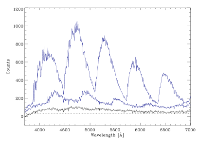
Figure 10: Example of a strong cross-talk effect in a fibre adjacent to a very bright source, in this case a standard star with a maximum of 40000 counts. The top spectrum shows the full cross-talk effect when no correction is applied. The middle spectrum shows a first-order correction obtained by minimising the pixel extraction aperture (but losing flux in the process). The bottom spectrum shows the correction of the cross-talk by the improved Gaussian-suppression method (described in Paper II) with an extracted spectrum of the same order of intensity as the average background signal (dotted line) found in the nearby fibres for this particular observation. The apparent periodicity of the cross-talk with respect to the wavelength is just an effect of the spectra misalignments and distortions on the CCD.

6.5 Cross-talk

One of the critical reduction steps is to extract the flux corresponding to different spectra at each pixel along the dispersion axis (see section 5). However, this is not straightforward as there could be contamination by flux coming from the adjacent spectra, i.e. cross-talk. This contamination effect may produce a wrong interpretation of the data. For observations performed with PPAK, and due to the geometrical construction of the instrument, the adjacent spectra on the plane of the CCD may not correspond to nearby locations in the sky plane (Kelz et al., 2006). Furthermore, the position of the calibration fibres (which are located in between the science ones along the pseudo-slit) also contributes to overall contamination. Therefore, the cross-talk effect would potentially mix up spectra from locations that may not be physically related (because of the spectra position on the CCD) or from spectra with completely different nature (i.e. calibration fibres). Given that the cross-talk is an incoherent contamination it is preferable to keep it as low as possible, an average value of $\sim$ 1% with a maximum of $\sim$ 10% ( San06, and references therein) seems technically as a good trade-off.

Given the limited size of CCDs and the need to record as many spectra as possible within that reduced area, IFS observations will always face a certain level of cross-talk. The FWHM of the projected profile along the cross-dispersion axis is normally defined by the design of the spectrograph and the size of the input fibres, placing a limit in the selected aperture. As explained by San06, the PPAK spectra profiles have a FWHM of the order of $\sim$ 2.3 pixels, and $\Delta$ peaks of $\sim$ 5 pixels in the 2 $\times$ 2 binning mode (as was the case for all PINGS observations). Selecting an aperture size of the order of $\Delta$ peaks seems to be an acceptable compromise between maximising the recovered flux and minimising the cross-talk. Several methods have been implemented to minimise the effect of cross-talk, in particular, San06 developed an efficient technique named Gaussian-suppression that reduces the effects of the cross-talk and maximises the recovered flux to within 10% of the original values for any spaxel at any wavelength. However, for certain raw frames which were too crowded or when we targeted bright sources within the field (e.g. foreground stars, galaxy bulges), we still found some level of contamination that could not be considered negligible.

Therefore, we improved the Gaussian-suppression technique to a new method which increases the signal-to-noise ratio of the extracted spectra and reduces the effect of the cross-talk compared to previous extractions. The new technique is explained in detail in Paper II, and it is now fully implemented in the standard R3D package (San06). We performed several tests using simulated and real spectra with a broad range of intensities in order to assess the level of contamination that the extracted spectra show due to the cross-talk. We tested the new method varying the relative intensity of the spectra in the central and adjacent fibres, the pixel extraction apertures and the average width of the Gaussian profiles. We found that in the extreme cases (very bright adjacent fibres) the cross-talk is suppressed by 95%, being almost negligible for the range of spectral intensities compared to the instrumental misalignments and distortions found during conventional observations of the PINGS sample (see Figure 10).

In summary, the two most important sources of error in the data reduction arise from the sky subtraction and the flux calibration. We have made several tests and applied new techniques in each case in order to minimise the magnitude of the uncertainties. We found that the sky subtraction cannot be applied as part of any standard reduction pipeline and has to be considered on an individual basis, depending on the observing mode, configuration and strategy. On the other hand, the maximum expected error in the absolute flux calibration for those objects in which a broad-band imaging recalibration was applied is of the order of 20%, being slightly larger in a narrow blue spectral region $\lambda<$ 3800 Å. For those objects without broad-band imaging, the absolute flux calibration error is of the order of 30%. However, the absolute error is better than 20% for objects observed during photometric conditions and/or with high S/N. The colors, spectral features and gradients are completely reproduced when comparing our data with previously published long-slit observations (see subsection 7.1).

DAR effects were found to be negligible due to the large size of the spatial elements of PPAK, we did not find strong evidence of DAR in the several test pointings analysed. However we flagged all individual IFU positions for which the observations were performed with an airmass $>$ 1.3. With respect to cross-talk, the new extraction method proved to suppress this effect to a negligible level for the range of spectral intensities in the PINGS observations. Furthermore, no evidence of any second-order contamination has been found during the data reduction and analysis of the PINGS data set. As explained in section 4, the contamination of the 2nd order, up to 7200 Å, is expected to be lower than 1/10000, being negligible for our science case.

7 The PINGS data

The PINGS data set contains more than 50000 flux calibrated spectra for a sample of 17 galaxies covering in total an observed spectroscopic area of nearly 80 arcmin². subsection 4.3 shows a summary of the observations, including the number of individual IFU pointings observed for the mosaic of each galaxy, the observational status of the mosaicking, the total number of spectra, and additional individual comments on each object. The spectroscopic data set samples the observed objects with fibre circular apertures of $\sim$ 2.7 arcsec in diameter, covering the optical wavelength range between $\sim$ 3700 – 7100 Å, which includes the most prominent recombination and collisionally excited emission lines from [O II] $\lambda$$\lambda$ 3727, 3729 to [S II] $\lambda$$\lambda$ 6717, 6731.

It is beyond the scope of this article to extract all the information potentially available in this huge spectroscopic data base. Independent studies for individual objects, regions and galaxy subsamples will be presented in a series of future papers. We consider here a few relevant scientific examples that have been extracted from the data set to demonstrate the use of these data. In this section we present the integrated spectra and emission line intensities for selected H II regions of the IFS mosaics of NGC 1058 and NGC 3310, with a comparison to previously published data. Furthermore, we obtained emission line maps for NGC 1058 and we present a qualitative description of the 2D distribution of physical properties inferred from the line intensity maps. Finally, we present the spectra of the SN 2007gr observed in NGC 1058 as an example of the utility of wide-field IFS surveys to find potential SNe progenitors and their environmental properties.

7.1 Integrated spectra

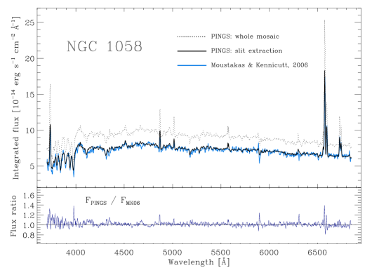
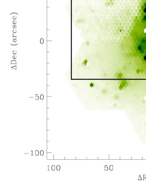
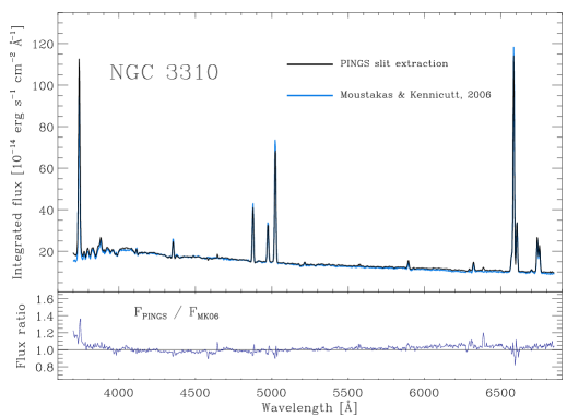
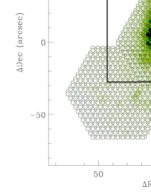
Figure 11: Top panels: Integrated spectra of NGC 1058 derived from the PINGS slit-extraction (thick solid line) and the whole mosaic (dotted line) spectra compared to the MK06 data (blue line in the online version), as explained in the text. Flux in units of 10^-16 erg s^-1 cm^-2 Å^-1. Bottom panels: Comparison of the integrated spectra of NGC 3310 with the same color coding as the figure above. For both galaxies, the diagrams on the right represent narrow-band intensity maps centred at H$\alpha$ showing the mosaic pattern and the rectangular slit-apertures of MK06. The arrow in the NGC 1058 mosaic diagram shows the position of SN 2007gr. The contours of the individual fibres have been drawn in the case of NGC 3310.

The study of the optical integrated light provides a powerful tool to investigate the physical properties of galaxies at different epochs in the history of the universe. Spectral investigations based on integrated optical spectrophotometry have been used to explore the main drivers of galaxy evolution, e.g. star formation rate, star formation history, stellar mass, chemical abundance, dust content, etc. (e.g. Kauffmann et al., 2003; Tremonti et al., 2004). The analysis of the integrated spectra in nearby objects can be used to assess the limitations imposed by high-redshift surveys, such as their limiting magnitude and incomplete spatial coverage (or aperture bias), factors that may be important given that many physical properties of galaxies vary depending on the geometry and position (e.g. stellar populations, metallicity, extinction, etc.). A solution to the incomplete spatial coverage of spectroscopic observations on nearby objects consists on using sequential methods that use time to scan a target while recording the spectral information. The standard method for obtaining integrated spectra in nearby objects was developed by Kennicutt (1992). The so-called drift-scanning technique consists of a scan perpendicular to the slit over the optical extent of the galaxy during a single exposure. Using this method Moustakas & Kennicutt 2006b (hereafter MK06) obtained spatially integrated optical (3600 – 6900 Å) spectrophotometry for 417 nearby galaxies of a diverse range of galaxy types, which were later used to study several integrated galactic properties (SFR, metallicity, etc.).

One by-product of 2D spectroscopy and IFS data sets is the intrinsic capability of adding up all the spectra within an observed field or mosaic into a single spectrum, i.e. using the IFU as a large-aperture spectrograph to obtain the integrated spectra of a given FOV. The PINGS sample is an ideal data set for this purpose given that the spectroscopic mosaics cover, in most cases, the entire optical radius of the galaxy. The integrated spectra derived from PINGS can be used to study the real average spectroscopic properties of a given nearby, large angular size galaxy, as opposed to previous studies that attempted to describe their average properties by the analysis of individual spectra taken from different regions, or by targeting objects with a limited extraction aperture which recovers only a fraction of the total optical light. In this section we present examples of high signal-to-noise integrated spectra for NGC 1058 and NGC 3310 obtained by co-adding the spectra from their corresponding mosaics using different simulated apertures applied to the IFS mosaic. We compare these data with previously published integrated spectra from MK06. In Paper II, we present the integrated spectra of NGC 628 with a more elaborated analysis of the integrated stellar populations and nebular abundances.

Figure 11 shows in the left upper panel the comparison of the integrated spectrum of NGC 1058 extracted from the PINGS mosaic to the drift-scan spectrum obtained by MK06 of this galaxy, at the same spectral resolution. The right upper panel shows the PINGS spectroscopic mosaic diagram of NGC 1058 with intensity levels corresponding to a “narrow-band” 100 Å width image extracted from the IFS data centred at H$\alpha$. The rectangular shape shows the slit-aperture used in the drift-scan technique by MK06 to obtain the integrated spectrum of this galaxy. Three foreground stars and the supernova SN 2007gr (see subsection 7.4) were removed from the co-added spectra (the arrow shows the position of SN 2007gr between two foreground stars). The black solid line spectrum in the left upper panel was obtained by extracting from the PINGS mosaic all the individual spectra within the area enclosed by the rectangular shape and taking into account the overlapping regions and the covering fraction of the fibres due to the dithering technique applied to this galaxy.

The blue line corresponds to the spectrum obtained by MK06 using the drift-scan technique. The dotted line was derived after co-adding all the spectra of the seven IFU positions shown in Figure 11 and considering the dithering overlaps. This spectrum is constructed out of 6951 individual spectra covering the whole optical $B_{25}$ mag arcsec^-2 radius of NGC 1058. In this case we can see clearly the effect of the incomplete spatial coverage when comparing the integrated spectrum within the slit-aperture of MK06 and the whole optical radius covered by the PINGS mosaic (dotted line). Although it is beyond the scope of this paper to give a more quantitative comparison, we can notice from a purely qualitative point of view that the determination of some physical properties may vary when using both the slit-aperture and the whole mosaic integrated spectra, probably by as much as $\sim$ 15 – 20%.

In a similar way, the bottom panels of Figure 11 show the integrated spectra of the starburst galaxy NGC 3310. The black line shows the integrated spectrum obtained after co-adding all the spectra within the rectangular pattern corresponding to the MK06 slit-aperture and considering all the overlaps in the mosaic due to the dithering observing method and the non-standard construction of the mosaic. No foreground stars were found within this field. The blue line corresponds to the MK06 drift-scan integrated spectrum. In this case the PINGS extraction is spatially incomplete when compared to the rectangular area of the MK06 aperture. Nevertheless, all the spectral features are reproduced quite well when we compare the PINGS spectrum with the MK06 data. The apparent disagreement seen in some of the emission lines can be explained by the spatial incompleteness of the IFS mosaic with respect to the MK06 slit, and the presence of a bright H II region at ($\Delta\alpha$, $\Delta\delta$) $\sim$ (–10,–30), which is located at the edge of the extraction slit and presents particularly strong emission in the [O III] lines. A small shift of the reported position of the MK06 slit results in a slightly different integrated spectrum due to this strong H II region, causing that the peaks of the emission lines differ in height. A stronger effect is seen in the blue spectral region ($\lambda<$ 3800 Å) which is expected due to the intrinsic problems of the spectrophotometric calibration in this regions as explained in section 6. The integrated spectrum of NGC 3310 using all the fibres in the three dithered positions differs very little from the extracted one, and it is not shown for the sake of clarity.

The spectroscopic mosaics of NGC 1058 and NGC 3310 were not re-calibrated using the broad-band imaging technique described in Paper II, and therefore they are not calibrated for the absolute zero point flux. Nevertheless, both the spectral shape and the spectral features of the PINGS extracted spectra corresponding to the slit-aperture of MK06 match remarkably well with these previously published, spectrophotometrically calibrated data, showing the quality of the PINGS IFS data set.

7.2 Emission line maps

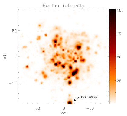
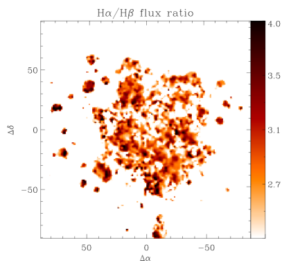
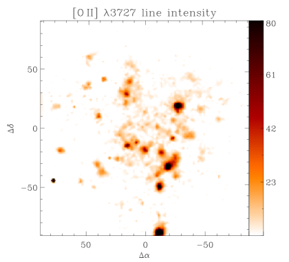
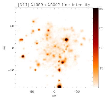
Figure 12: Emission line maps obtained from the IFS mosaic of NGC 1058 (without the outlying pointing). In the top-left panel, H$\alpha$ line intensity map, top-right H$\alpha$/H$\beta$ flux line ratio. Bottom-left, [O II] $\lambda$3727, bottom-right [O III] $\lambda$4959 + $\lambda$5007 intensity maps. All maps were obtained by fitting a single Gaussian function to the emission line for each single spectrum in the mosaic. The intensity map is then reconstructed by interpolating the recovered flux at the location of each spectrum as described in the text. All maps are in units of 10^-16 erg s^-1 cm^-2 arcsec^-2. No correction for dust extinction was applied to any map.

One of the main objectives of the PINGS project is to obtain complete maps of the emission-line intensities which could then be analysed to describe the 2D spatially-resolved distribution of the physical properties of the sample. The PINGS spectroscopic mosaics allow us to obtain for the first time a complete 2D view in the optical wavelength range of the main emission lines used in typical abundance diagnostics methods, and important spectral features useful for the analysis of the underlying stellar populations.

The ionized gas in spiral galaxies exhibits a complex structure associated morphologically with star-forming regions located mainly along the spiral arms. Previous attempts to perform a 2D analysis have made use of narrow-band and Fabry-Perot imaging at different spectral widths. However, in some cases the narrow-band imaging includes the contribution of more than one single emission line, such as the case of the H$\alpha$ imaging, which includes the [N II] $\lambda\lambda$ 6548, 6584 doublet, or the [S II] density sensitive doublet at $\lambda\lambda$ 6717, 6731. This factor limits the utilization of these techniques to study just the basic parameters of the ionized gas, under the assumption of fixed line ratios. The great advantage of IFS arises from the fact that we are able to deblend emission lines at any discrete spatial location, and to ultimately produce maps of individual emission lines.

In order to extract any physical information from the data set, we need first to identify the detected emission lines of the ionized gas and to decouple their emission from the stellar population in each individual spectrum of the IFS mosaic. We used population synthesis to model and subtract the stellar continuum underlying the nebular emission lines. This technique results in emission-line measurements corrected (to a first-order) for stellar absorption. The details of this process are described in Paper II, however we present briefly here the scheme followed to decouple the stellar population and the emission lines in our database: i) A set of emission lines is identified from any strong H II region of the galaxy. ii) For each spectrum in the data set, the underlying stellar population is fitted by a linear combination of a grid of Single Stellar Populations (SSP), masking all the nebular and sky emission lines. The template models are selected in order to cover the widest possible range of ages and metallicities. We consider the effects of dust extinction by varying A_V from 0 to 1 mag at $\Delta$ 0.2 mag. iii) We subtract the fit stellar population from the original spectrum to get a residual pure emission-line spectrum. iv) Finally, we derive the intensities for each detected emission line.

Individual emission-line fluxes were measured in each spectrum by considering spectral window regions of $\sim$ 200 Å. We performed a simultaneous multi-component fitting using a single Gaussian function (for each emission line contained within each window) plus a low order polynomial (to describe the local continuum and to simplify the fitting procedure) using FIT3D (Sánchez et al., 2006). The central redshifted wavelengths of the emission lines were fixed and since the FWHM is dominated by the spectral resolution, the widths of all the lines were set equal to the width of the brightest line in this spectral region. This procedure decreases the number of free parameters and increases the accuracy of the deblending process (when required). Line intensity fluxes were then measured by integrating the observed intensity of each line. The statistical uncertainty in the measurement of the line flux was calculated by propagating the error associated to the multi-component fitting and considering the signal-to-noise of the spectral region.

We applied this line-fitting method to NGC 1058 and created emission line maps by interpolating the intensities derived for each individual line in each individual spectrum, correcting for the dithering overlapping effects. The interpolation was performed using E3D, adopting a natural-neighbour, non-linear interpolation scheme, with a final scale of 1”/pixel in the resulting maps. The data at the location of bright foreground stars in the field were masked prior to any interpolation, in order to decrease the effects of their contamination.

As a prime example of this technique for the purpose of this paper, we calculated the following emission line maps: H$\alpha$, H$\beta$, the doublet-blended [O II] $\lambda$3727, and [O III] $\lambda\lambda$ 4959, 5007. In order to prevent contamination by low signal-to-noise data, we masked all pixels that correspond to an integrated flux per fibre below 10^-16 erg s^-1 cm^-2. Figure 12 shows the emission line maps in units of 10^-16 erg s^-1 cm^-2 arcsec^-2. The top panels show the distribution of the star-forming regions in the galaxy traced by the H$\alpha$ intensity map (left) and the distribution of dust extinction, outlined by the H$\alpha$/H$\beta$ flux ratio (right). From these maps we note that, although many of the most intense emission regions are located along the inner spiral arms of the galaxy, some of them lie in outer regions not associated with any spiral structure (e.g. to the south of the galaxy, at $\Delta$RA $\sim$ –10, $\Delta$Dec $\sim$ –90 arcsec). On the other hand, the H$\alpha$/H$\beta$ flux ratio shows a smooth distribution, especially concentrated in the inner part of the galaxy with strong peaks in the outlying star-forming regions. As a matter of fact, the very intense outlying regions of star-formation are responsible for the difference found in between the integrated spectra of NGC 1058 when comparing the central slit-aperture of MK06 to the whole mosaic (see subsection 7.1). NGC 1058 is known to have a larger than average H I-to-optical size, and deep H$\alpha$ imaging has revealed the existence of recent massive star formation out to and beyond two optical radii (Ferguson et al. 1998, hereafter FGW98). However, the small number of H II regions analysed in previous studies of NGC 1058 has prevented a complete explanation of the existence of these extreme outer regions, and of the intrinsic scatter of the abundance gradient seen in this galaxy. Given the spatial information provided by the PINGS spectroscopic mosaic, we could in principle study the properties of the outer H II regions with those of the inner disk and test the predictions of chemical evolution models and the behavior of the chemical abundances not only as a function of increasing radius, but taking into consideration the morphology of the galaxy.

The bottom panels show the line intensity distribution of [O II] $\lambda$3727 (left), and [O III] $\lambda$4959 + $\lambda$5007 (right). For both cases, we notice strong emission regions at $\Delta$RA $\sim$ –20 arcsec, and again several outlying emission regions that do not follow the spiral pattern of the galaxy. More definite interpretations than the qualitative ones described here can be achieved with a full spectroscopic analysis of the dust content, ionization conditions and metallicity distribution of the the whole IFS mosaic.

Table 3: Comparison of the PINGS emission line intensities for two H II regions in NGC 1058 and one in NGC 3310 with previous observations and published line ratios. For NGC 1058 we compare with the regions E and H by Ferguson et al. (1998), and the Jumbo H II region in NGC 3310 observed by Pastoriza et al. (1993). For NGC 1058, the coordinates shown represent approximate offsets of the H II regions with respect to the galaxy nucleus in the PINGS mosaic in the format ($\Delta$RA, $\Delta$Dec) with NE positive. All values for NGC 1058 are the observed line ratios. In the case of the NGC 3310 Jumbo H II region, the observed and redenning corrected ratios for PINGS are shown as Pas 93 only shows corrected line intensities (see text for details). All line ratios are normalised to H$\beta$. * Observed H$\beta$ flux in units of 10^-16 erg s^-1 cm^-2.

	NGC 1058					NGC 3310 Jumbo H II region
	(–10.6, –87.9)		(140.6, 90.0)			PINGS		Pas 93
Line	PINGS	FGW 1058E	PINGS	FGW 1058H		F($\lambda$)/F(H$\beta$)	I($\lambda$)/I(H$\beta$)	I($\lambda$)/I(H$\beta$)
[O II]  $\lambda$3727	3.033 $\pm$ 0.262	2.739 $\pm$ 0.064	2.261 $\pm$ 0.130	1.950 $\pm$ 0.052		2.388 $\pm$ 0.132	3.028 $\pm$ 0.352	2.59 $\pm$ 0.040
[Ne III]  $\lambda$3869	0.170 $\pm$ 0.018		0.188 $\pm$ 0.026			0.180 $\pm$ 0.020	0.223 $\pm$ 0.048	0.18 $\pm$ 0.040
H8 + He I  $\lambda$3889	0.164 $\pm$ 0.018		0.111 $\pm$ 0.021			0.126 $\pm$ 0.021	0.156 $\pm$ 0.044	0.13 $\pm$ 0.039
H$\epsilon$  $\lambda$3970	0.162 $\pm$ 0.018		0.173 $\pm$ 0.025			0.115 $\pm$ 0.020	0.140 $\pm$ 0.043	0.17 $\pm$ 0.053
H$\delta$  $\lambda$4101	0.209 $\pm$ 0.022		0.228 $\pm$ 0.029			0.184 $\pm$ 0.020	0.218 $\pm$ 0.039	0.21:
H$\gamma$  $\lambda$4340	0.386 $\pm$ 0.039		0.447 $\pm$ 0.046			0.406 $\pm$ 0.018	0.455 $\pm$ 0.046	0.40:
[O III]  $\lambda$4363	…		…			0.017 $\pm$ 0.004	0.019 $\pm$ 0.006	0.018 $\pm$ 0.005
He I  $\lambda$4471	0.029 $\pm$ 0.004		0.052 $\pm$ 0.012			0.034 $\pm$ 0.004	0.037 $\pm$ 0.009	0.036 $\pm$ 0.009
H$\beta$  $\lambda$4861	1.000 $\pm$ 0.050	1.000 $\pm$ 0.033	1.000 $\pm$ 0.051	1.000 $\pm$ 0.037		1.000 $\pm$ 0.038	1.000 $\pm$ 0.082	1.000 $\pm$ 0.053
[O III]  $\lambda$4959	0.745 $\pm$ 0.038	0.786 $\pm$ 0.026	1.137 $\pm$ 0.057	1.148 $\pm$ 0.042		0.936 $\pm$ 0.048	0.919 $\pm$ 0.067	0.740 $\pm$ 0.007
[O III]  $\lambda$5007	2.301 $\pm$ 0.115	2.298 $\pm$ 0.076	3.227 $\pm$ 0.163	3.282 $\pm$ 0.117		2.857 $\pm$ 0.060	2.779 $\pm$ 0.143	2.310 $\pm$ 0.009
He I  $\lambda$5876	0.109 $\pm$ 0.011		0.223 $\pm$ 0.024			0.133 $\pm$ 0.011	0.114 $\pm$ 0.013	0.099 $\pm$ 0.005
[O I]  $\lambda$6300	0.050 $\pm$ 0.006		0.069 $\pm$ 0.009			0.060 $\pm$ 0.008	0.050 $\pm$ 0.010	0.051 $\pm$ 0.004
[S III]  $\lambda$6312	…		…			0.011 $\pm$ 0.004	0.009 $\pm$ 0.006	0.011 $\pm$ 0.003
[O I]  $\lambda$6363	…		…			0.021 $\pm$ 0.006	0.017 $\pm$ 0.008	0.014 $\pm$ 0.005
[N II]  $\lambda$6548	0.142 $\pm$ 0.023	0.135 $\pm$ 0.005	0.065 $\pm$ 0.013	0.099 $\pm$ 0.009		0.189 $\pm$ 0.018	0.152 $\pm$ 0.020	0.150 $\pm$ 0.005
H$\alpha$  $\lambda$6563	3.114 $\pm$ 0.156	3.231 $\pm$ 0.106	3.135 $\pm$ 0.158	2.980 $\pm$ 0.106		3.574 $\pm$ 0.056	2.870 $\pm$ 0.179	2.880 $\pm$ 0.004
[N II]  $\lambda$6584	0.413 $\pm$ 0.045	0.414 $\pm$ 0.014	0.187 $\pm$ 0.022	0.179 $\pm$ 0.009		0.548 $\pm$ 0.038	0.439 $\pm$ 0.055	0.460 $\pm$ 0.003
He I  $\lambda$6678	0.037 $\pm$ 0.004		0.020 $\pm$ 0.006			0.045 $\pm$ 0.006	0.035 $\pm$ 0.008	0.032 $\pm$ 0.003
[S II]  $\lambda$6717	0.373 $\pm$ 0.028	0.362 $\pm$ 0.012	0.190 $\pm$ 0.020	0.238 $\pm$ 0.011		0.315 $\pm$ 0.014	0.249 $\pm$ 0.032	0.270 $\pm$ 0.006
[S II]  $\lambda$6731	0.270 $\pm$ 0.023	0.257 $\pm$ 0.009	0.134 $\pm$ 0.014	0.148 $\pm$ 0.008		0.248 $\pm$ 0.015	0.196 $\pm$ 0.025	0.220 $\pm$ 0.006
I($\lambda$5007)/I($\lambda$4959)	3.09 $\pm$ 0.15	2.92 $\pm$ 0.14	2.83 $\pm$ 0.20	2.85 $\pm$ 0.15		3.05 $\pm$ 0.05	3.02 $\pm$ 0.08	3.12 $\pm$ 0.03
* F(H$\beta$)  $\lambda$4861	236.2	210.5	11.6	19.5		1096		1690

7.3 Emission line ratios: comparison with literature

Several galaxies in the PINGS sample have been spectroscopically studied previously by different authors. As a consistency test of the quality of our data we performed a comparison of several emission line ratios as measured by the procedure described in the previous section with selected H II regions from the literature for which the authors published the emission line ratios for different species. Table 3 shows a comparison of the PINGS emission line intensities for three of those regions: FGW 1058E and FGW 1058H, analysed by FGW98, and the Jumbo H II region in NGC 3310 observed by Pastoriza et al. 1993, (hereafter Pas93).

FGW98 observed a total of 8 H II regions in NGC 1058, however, regions FGW 1058A to D are located in the inner part of the galaxy and their identification is somewhat unclear (see Figure 2 from FGW98). Regions FGW 1058F and FGW 1058G fall outside the observed FOV of PINGS. On the other hand, FGW 1058E is a bright H II region located at $\sim$ (–10, –88) arcsec in ($\Delta$RA, $\Delta$Dec) units with respect to the galaxy centre (see Figure 12), while FGW 1058H is an outlying H II region located at $\sim$ (140, 90) in the PINGS mosaic (see Figure 2). For this comparison we selected these two objects as both fall within the FOV observed by PINGS and are uniquely distinguishable from the H$\alpha$ maps/images.

In the case of FGW 1058, we used for this comparison a 4 arcsec circular aperture centered on the fibre with the strongest emission in H$\alpha$, assuming that the long-slit observation was placed in this region as FGW98 did not give details of the observation of each specific object and their given offsets are only approximate with respect to the centre of the galaxy (even the extraction aperture is uncertain as they only quote a size range from 3 to 15 arcsec depending on the seeing and on the size of the object in question). In the case of FGW 1058H, the identification was relatively simple as this is a small and well-defined outlying H II region. The emission line ratios for this region were obtained from a single fibre at the quoted position. FGW98 published the observed and reddening corrected emission line intensities for 9 spectral lines, in Table 3 we compare our results with the observed un-corrected emission line fluxes only. Additional spectral lines and atomic species detected and measured in the PINGS data are also included in Table 3.

Pas93 performed an optical and near-IR spectroscopic analysis of circumnuclear H II regions (at less than 400 pc from the nucleus) and the Jumbo H II region in NGC 3310. The identification of the circumnuclear H II regions is somewhat difficult in the PINGS mosaic given the linear scale of the regions and the size of the fibres. Therefore we chose to analyse the bright Jumbo H II region for which emission line intensities were measured by Pas93. The slit position, aperture and PA are well described by these authors, however we did not choose to simulate an aperture in the PINGS mosaic as the aperture of the slit used by Pas93 (1.5 arcsec) is smaller than the size of a single PPAK fibre. Instead, we chose the fibre within this region with the strongest emission in H$\alpha$, which corresponds to an offset (–10.6, –2.2) in ($\Delta$RA, $\Delta$Dec) with respect to the galaxy centre in the PINGS mosaic.

Pas93 quoted only the reddening corrected line intensities, therefore for this comparison, Table 3 shows the observed and reddening corrected line ratios obtained from the PINGS spectrum extracted for this region. The PINGS observed line intensities listed in Table 3 were corrected for reddening using the Balmer decrement according to the reddening function of Cardelli et al. (1989), assuming $R\equiv A_{V}/E(B-V)=3.1$. Theoretical values for the intrinsic Balmer line ratios were taken from Osterbrock & Ferland (2006), assuming case B recombination, an electron density of $n_{e}=100$ cm^-3 and an electron temperature $T_{e}=10^{4}$ K. We have used only the H$\alpha$/H$\beta$ ratio to deduce the logarithmic reddening constant c(H$\beta$), obtaining a value of 0.32 for the PINGS spectrum, whereas Pas93 obtained c(H$\beta$) = 0.29 for the same region. We did not correct the emission line fluxes for underlying stellar absorptions. Formal errors in the derived line ratios were estimated by summing in quadrature the uncertainty in flux calibration, the statistical error in the measurement of the line flux and the error in the c(H$\beta$) term.

Despite the ambiguity due to the exact location and extraction aperture of the observed spectra, from Table 3 we can see that there is a very good agreement between the previously published emission line ratios and the PINGS observations for these three H II regions. The strongest deviation is found in the [O II] $\lambda$3727 as we expected, since this line falls in the spectral region at which the instrumental low sensitivity increases the flux calibration error. The comparison with the NGC 1058 regions is more straightforward as these are the observed values without any further correction. The comparison of the emission intensities with the NGC 3310 Jumbo H II region has to be made carefully since the values of Pas93 were corrected for underlying absorption and using a different reddening curve. Nevertheless, the reddening corrected values of PINGS are in good agreement with the values derived by Pas93, we even detected and measured correctly the very faint [O III] $\lambda$4363 line, showing the good quality of the sky subtraction despite the presence of the Hg $\lambda$4358 sky line. The line strength of the [O III] $\lambda$4363 line combined with the redshift of NGC 3310 makes it fall in the region of “detectability” as described in the simulation presented in subsection 6.2.

An additional assessment of the quality of the data is given by the value of the I($\lambda$5007)/I($\lambda$4959) ratio which can be predicted from atomic theory and observed in high signal-to-noise astronomical spectra. According to current atomic computations, the theoretical value for this intensity ratio is 2.98 (Storey & Zeippen, 2000). In Table 3 we show this ratio for the three H II regions. The observed central values for the region FGW 1058E in both datasets are in good agreement with the theoretical value. In the case of FGW 1058H both values are quite similar but differ within the errors from the theoretical value. For the NGC 3310 Jumbo H II region, the central value observed by PINGS is closer to the theoretical value for both uncorrected and corrected line ratios compared to the Pas93 value.

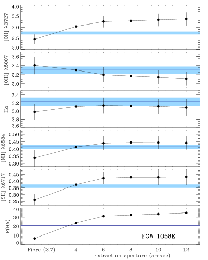
Figure 13: Variation of the emission line ratios as a function of integration aperture of the H II region FGW 1058E. The horizontal line/band in each panel shows the value/error derived by FGW98. All emission line intensities are normalized to H$\beta$. The observed integrated fluxes of H$\beta$ are in units of 10^-15 erg s^-1 cm^-2.

The flux observed by PINGS in the H$\beta$ line for FGW 1058E is slightly higher than the one measured by FGW98, contrary to the case of FGW 1058H, where the flux in PINGS for the same line is somehow smaller, reflecting the unknown aperture extraction for the FGW98 long-slit spectrum. In the case of the NGC 3310 Jumbo H II region, the flux measured by PINGS is somewhat smaller than the one measured by Pas93.

The 2D character of the PINGS data allows us to study the variation of the spectra within a given area that would be otherwise taken as a single H II region. In Figure 13 we show the effect of the extraction aperture on the emission line intensities for the H II region FGW 1058E. FGW98 considered FGW 1058E as a single H II region, however a closer look using the dithered spectroscopic mosaic shows that this region is actually a complex composed of several knots and substructures with varying emission fluxes in the most prominent lines. In order to examine the difference in the emission line ratios in this region, we take as a central position the fibre with the strongest emission in H$\alpha$ within this area, with an integration aperture of 2.7 arcsec diameter. We then take concentric circular apertures of different sizes (ranging from 4 to 12 arcsec in diameter), we integrate the spectra within these apertures to obtain spectra from which we measure a different set of emission line intensities.

The five top panels of Figure 13 show the variation of the emission line ratios obtained at different extraction aperture sizes for some relevant lines (normalised to H$\beta$). The second data point corresponds to the value shown in Table 3 (4 arcsec aperture), the horizontal line in each panel shows the central value and the error bar obtained by FGW98 (the dark/light blue colour line/band in the online version). The bottom panel shows the integrated flux of H$\beta$ at each aperture. From Figure 13 we can see that the emission line ratios measured using different extraction apertures vary considerably as a function of the aperture size, and that in most cases the dispersion of the central values is larger than the error of the measurements, reflecting that this is a physical effect. All emission line ratios tend to converge to a certain value as the aperture size increases. Note that at the flux level in H$\beta$ measured by FGW98 for this region, all the emission line intensity ratios, as measured by PINGS, are basically the same (within errors) as the values derived by FGW98.

From this exercise we note that, to a first-order, the emission line ratios measured for a given H II region may significantly depend on the morphology of the region, on the slit (fibre) position, on the extraction aperture and on the signal-to-noise of the observed spectrum. All these effects should be taken into account when deriving physical quantities from spectroscopic studies of H II regions.

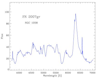
Figure 14: Extracted spectrum of the SN 2007gr in the mosaic of NGC 1058. The flux units are 10^-16 erg s^-1 cm² Å^-1. Some nebular emission lines are seen superimposed to the SN spectrum.

7.4 SN 2007gr in NGC 1058

As another example of the potential of the PINGS spectroscopic data, we present the spectrum of a particular object observed during the mosaicking of the galaxy NGC 1058. The observation of this galaxy was carried out during the nights of the 7th and 8th of December 2007. During this period we were able to observe the spectrum of the Supernova 2007gr, previously discovered by the Lick Observatory Supernova Search on the 15th of August 2007 (Chornock et al., 2007).

SN 2007gr was located at 24.8” West and 15.8” North of the nucleus of NGC 1058, with coordinates RA 02^h 43^m 27.^s98 and Dec: +37^∘ 20^m 44.^s7. In the mosaic diagram of NGC 1058 shown in Figure 11, the arrow shows the location of SN 2007gr between two bright foreground stars. Figure 14 shows the optical spectrum of the supernova extracted from the IFS mosaic, showing the typical spectrum of a Type Ic core collapse supernova, with the lack of hydrogen, helium and silicon absorption lines. Emission lines of [O II] $\lambda$3727, H$\alpha$, [N II] $\lambda$$\lambda$ 6548, 6584 and [S II] $\lambda$$\lambda$ 6717, 6731 are clearly seen on top of the SN spectra, probably reflecting the environment of the H II region in which this supernova exploded.

As described by Valenti et al. (2008), SN 2007gr showed an average peak luminosity but unusually narrow spectral lines and an almost flat photospheric velocity profile. SN 2007gr motivated an extensive observational campaign for several reasons: it was discovered at a very early stage (5 days after the explosion), it was located in a relatively close distance galaxy, it was the nearest stripped-envelope carbon-rich SNe ever observed, and a suitable candidate for progenitor search (Valenti et al., 2008). Wide-field IFS may become one of the main resources for SNe research groups to find SNe progenitors in previously observed galaxies. The progenitor supergiant stars ($M>$ 8 $M_{\odot}$) that at the end of their lives explode as core-collapse supernovae may show a strong stellar spectrum that could be recovered from 2D spectroscopic maps with enough spatial resolution. Furthermore, the nebular emission from the spatially adjacent spectra could provide information on the environment in which these SNe explosions occur.

8 Summary

We have presented the PPAK IFS Nearby Galaxies Survey: PINGS, a project designed to construct 2D spectroscopic mosaics of 17 nearby disk galaxies in the optical wavelength range. This project represents one of the first attempts to obtain continuous coverage spectra of the whole surface of a galaxy in the nearby universe.

The final sample includes different galaxy types, including normal, lopsided, interacting and barred spirals with a good range of galactic properties and SF environments with multi-wavelength public data. The spectroscopic data set comprises more than 50000 individual spectra, covering an observed area of nearly 80 arcmin². The data set will be supplemented with broad band and narrow band imaging for those objects without publicly available images in order to maximise the scientific and archival value of the observations. Future plans consider to release the PINGS data set in order to make it freely available to the scientific community as a PPAK legacy project.

The primary scientific objectives of PINGS are to obtain emission-line maps and moderate-resolution spectra of the underlying stellar population across the disks of the galaxies. These spectral maps will allow us to study the spatial distribution of the physical properties of the ionized gas and the stellar components in galaxies, solving the limitations imposed by the small FOV and spectral coverage of previous attempts at obtaining the 2D information of a galaxy. PINGS will provide the most detailed knowledge of star formation, gas chemistry and the variations across a late-type galaxy. This information is very relevant for interpreting the integrated colours and spectra of high redshift sources. The details provided by PINGS will contribute significantly to the study of the chemical abundances and the global properties of galaxies.

We have assessed very carefully all sources of errors and uncertainties found during the intrinsically complex reduction of IFS observations. This complexity is further deepened if one considers building an IFU spectroscopic mosaic of a given object for which the observations were performed at very different stages, for some objects even spanning a period of years.

To demonstrate the use of these data, we presented a few relevant scientific examples that have been extracted from the data set. We presented the integrated spectra of the IFS mosaics of NGC 1058 and NGC 3310 and a comparison with previously published data. Furthermore, we obtained emission line maps for NGC 1058 and we presented a qualitative description of the 2D distribution of physical properties inferred from the line intensity maps. We performed a comparison of the emission line ratios obtained for a number of selected H II regions from the literature, we showed that the emission line intensities obtained from the PINGS data agree with previously published studies, and that the line ratios derived from a single H II region may depend strongly on the position and aperture size of the slit/fibre (among other factors) for a given spectroscopic study. Finally, we showed the spectra of the SN 2007gr observed in NGC 1058 as an example of the utility of wide-field IFS surveys to find potential SNe progenitors and their environmental properties. Independent studies for individual objects, regions and galaxies samples will be presented in future papers. As a highlight of this project, the spectroscopic mosaicking of one of the sample objects: NGC 628, represents the largest area ever covered by an IFU observation. In Paper II we present a complete analysis of the integrated and spatially resolved properties of this galaxy.

Acknowledgments

FFRO would like to acknowledge the Mexican National Council for Science and Technology (CONACYT), the Dirección General de Relaciones Internacionales (SEP), Trinity College, the Cambridge Philosophical Society, and the Royal Astronomical Society for the financial support to carry out this research SFS and AD thank the Spanish Plan Nacional de Astronomía programmes AYA 2005-09413-C02-02 and AYA 2007-67965-C03-03 respectively. SFS acknowledges the Plan Andaluz de Investigación of Junta de Andalucía as research group FQM 360.

References

- Appleton et al. (2006) Appleton P. N., Xu K. C., Reach W., et al., 2006, ApJ, 639, L51
- Arribas et al. (1999) Arribas S., Mediavilla E., García-Lorenzo B., et al., 1999, A&AS, 136, 189
- Bacon et al. (2001) Bacon R., Copin Y., Monnet G., et al., 2001, MNRAS, 326, 23
- Balkowski et al. (1974) Balkowski C., Bottinelli L., Chamaraux P., et al., 1974, The Formation and Dynamics of Galaxies: Proceedings from IAU Symposium no. 58 held in Canberra, 58, 237
- Blanc et al. (2009) Blanc G. A., Heiderman A., Gebhardt K., et al., 2009, ApJ, 704, 842
- Bresolin (2006) Bresolin F., 2006, arXiv, p. 10
- Cardelli et al. (1989) Cardelli J. A., Clayton G. C., Mathis J. S., 1989, ApJ, 345, 245
- Chornock et al. (2007) Chornock R., Filippenko A. V., Li W., et al., 2007, CBET, 1036, 1
- Colless et al. (2001) Colless M., Dalton G., Maddox S., et al., 2001, Mon. Not. R. Astron. Soc., 328, 1039
- de Paz et al. (2005) de Paz A. G., Madore B. F., Boissier S., et al., 2005, ApJ, 627, L29
- de Vaucouleurs et al. (1991) de Vaucouleurs G., de Vaucouleurs A., Corwin H. G., et al., 1991, Third Reference Catalogue of Bright Galaxies (RC3)
- Diaz (1989) Diaz A. I., 1989, IN: Evolutionary phenomena in galaxies (A90-31743 13-90). Cambridge and New York, p. 377
- Drozdovsky & Karachentsev (2000) Drozdovsky I. O., Karachentsev I. D., 2000, A&AS, 142, 425
- Eastman et al. (1996) Eastman R. G., Schmidt B. P., Kirshner R., 1996, ApJ, 466, 911
- Falco et al. (1999) Falco E. E., Kurtz M. J., Geller M. J., et al., 1999, PASP, 111, 438
- Ferguson et al. (1998) Ferguson A. M. N., Gallagher J. S., Wyse R. F. G., 1998, AJ, 116, 673
- Filippenko (1982) Filippenko A. V., 1982, PASP, 94, 715
- Fisher et al. (1995) Fisher K. B., Huchra J. P., Strauss M. A., et al., 1995, ApJS, 100, 69
- Gallagher et al. (2001) Gallagher S. C., Charlton J. C., Hunsberger S. D., et al., 2001, AJ, 122, 163
- Garnett (2002) Garnett D. R., 2002, ApJ, 581, 1019
- Haynes et al. (1998) Haynes M. P., van Zee L., Hogg D. E., et al., 1998, AJ, 115, 62
- Hendry et al. (2005) Hendry M. A., Smartt S. J., Maund J. R., et al., 2005, MNRAS, 359, 906
- Hickson et al. (1992) Hickson P., de Oliveira C. M., Huchra J. P., et al., 1992, ApJ, 399, 353
- Izotov & Thuan (2004) Izotov Y. I., Thuan T. X., 2004, ApJ, 602, 200
- Jarrett et al. (2003) Jarrett T. H., Chester T., Cutri R., et al., 2003, AJ, 125, 525
- Karachentsev et al. (2002) Karachentsev I. D., Dolphin A. E., Geisler D., et al., 2002, A&A, 383, 125
- Kauffmann et al. (2003) Kauffmann G., Heckman T. M., White S. D. M., et al., 2003, Monthly Notice of the Royal Astronomical Society, 341, 33
- Kehrig et al. (2008) Kehrig C., Vílchez J. M., Sánchez S. F., et al., 2008, A&A, 477, 813
- Kelz & Roth (2006) Kelz A., Roth M. M., 2006, NewAR, 50, 355
- Kelz et al. (2006) Kelz A., Verheijen M. A. W., Roth M. M., et al., 2006, PASP, 118, 129
- Kennicutt (1992) Kennicutt R. C., 1992, ApJS, 79, 255
- Kennicutt et al. (2003) Kennicutt R. C., Armus L., Bendo G., et al., 2003, PASP, 115, 928
- Kennicutt & Garnett (1996) Kennicutt R. C., Garnett D. R., 1996, ApJ, 456, 504
- Kent (1981) Kent S. M., 1981, Astronomical Society of the Pacific, 93, 554
- Kregel & Sancisi (2001) Kregel M., Sancisi R., 2001, A&A, 376, 59
- Leonard et al. (2002) Leonard D. C., Filippenko A. V., Li W., et al., 2002, AJ, 124, 2490
- Lu et al. (1993) Lu N. Y., Hoffman G. L., Groff T., et al., 1993, ApJS, 88, 383
- McCall et al. (1985) McCall M. L., Rybski P. M., Shields G. A., 1985, ApJS, 57, 1
- Marquez et al. (1996) Marquez I., Moles M., Masegosa J., 1996, A&A, 310, 401
- Martin & Roy (1994) Martin P., Roy J.-R., 1994, ApJ, 424, 599
- Moustakas & Kennicutt (2006a) Moustakas J., Kennicutt R. C., 2006a, ApJ, 651, 155
- Moustakas & Kennicutt (2006b) Moustakas J., Kennicutt R. C., 2006b, ApJS, 164, 81
- Nakano & Kushida (1999) Nakano S., Kushida R., 1999, IAU Circ., 7329, 1
- Nishiura et al. (2000) Nishiura S., Shimada M., Ohyama Y., et al., 2000, AJ, 120, 1691
- Nordgren et al. (1997) Nordgren T. E., Chengalur J. N., Salpeter E. E., et al., 1997, Astronomical Journal v.114, 114, 77
- Oke (1990) Oke J. B., 1990, AJ, 99, 1621
- Osterbrock & Ferland (2006) Osterbrock D. E., Ferland G. J., 2006, Astrophysics of gaseous nebulae and active galactic nuclei
- Pagel et al. (1992) Pagel B. E. J., Simonson E. A., Terlevich R. J., et al., 1992, MNRAS, 255, 325
- Pastoriza et al. (1993) Pastoriza M. G., Dottori H. A., Terlevich E., et al., 1993, MNRAS, 260, 177
- Pettini (2006) Pettini M., 2006, The Fabulous Destiny of Galaxies: Bridging Past and Present. Marseille International Cosmology Conference (5 : 2005: Marseille, p. 319
- Roberts et al. (2001) Roberts M. S., Hogg D. E., Schulman E., 2001, Gas and Galaxy Evolution, 240, 294
- Rosolowsky & Simon (2008) Rosolowsky E., Simon J. D., 2008, ApJ, 675, 1213
- Roth et al. (2005) Roth M. M., Kelz A., Fechner T., et al., 2005, PASP, 117, 620
- Roy & Walsh (1988) Roy J.-R., Walsh J. R., 1988, MNRAS, 234, 977
- Saha et al. (2006) Saha A., Thim F., Tammann G. A., et al., 2006, ApJS, 165, 108
- Sánchez (2004) Sánchez S. F., 2004, AN, 325, 167
- Sánchez (2006) Sánchez S. F., 2006, AN, 327, 850
- Sánchez et al. (2007) Sánchez S. F., Aceituno J., Thiele U., et al., 2007, PASP, 119, 1186
- Sánchez et al. (2007a) Sánchez S. F., Cardiel N., Verheijen M. A. W., et al., 2007a, Mon. Not. R. Astron. Soc., 376, 125
- Sánchez et al. (2007b) Sánchez S. F., Cardiel N., Verheijen M. A. W., et al., 2007b, A&A, 465, 207
- Sánchez et al. (2006) Sánchez S. F., García-Lorenzo B., Jahnke K., et al., 2006, AN, 327, 167
- Sánchez et al. (2009) Sánchez S. F., Rosales-Ortega F. F., Kenniccutt R., et al., 2009, submitted
- Sandin et al. (2008) Sandin C., Schönberner D., Roth M. M., et al., 2008, A&A, 486, 545
- Scowen et al. (1996) Scowen P. A., Hester J. J., Gallagher J. S., et al., 1996, BAAS, 189, 1360
- Skillman et al. (1989) Skillman E. D., Kennicutt R. C., Hodge P. W., 1989, ApJ, 347, 875
- Smith et al. (1999) Smith D. A., Herter T., Haynes M. P., et al., 1999, ApJ, 510, 669
- Springob et al. (2005) Springob C. M., Haynes M. P., Giovanelli R., et al., 2005, ApJS, 160, 149
- Storey & Zeippen (2000) Storey P. J., Zeippen C. J., 2000, Mon. Not. R. Astron. Soc., 312, 813
- Terry et al. (2002) Terry J. N., Paturel G., Ekholm T., 2002, A&A, 393, 57
- Theureau et al. (1998) Theureau G., Bottinelli L., Coudreau-Durand N., et al., 1998, A&AS, 130, 333
- Tremonti et al. (2004) Tremonti C. A., Heckman T. M., Kauffmann G., et al., 2004, ApJ, 613, 898
- Valenti et al. (2008) Valenti S., Elias-Rosa N., Taubenberger S., et al., 2008, ApJ, 673, L155
- van Zee et al. (1998) van Zee L., Salzer J. J., Haynes M. P., 1998, ApJ, 497, L1
- Verheijen et al. (2004) Verheijen M. A. W., Bershady M. A., Andersen D. R., et al., 2004, AN, 325, 151
- Vila-Costas & Edmunds (1992) Vila-Costas M. B., Edmunds M. G., 1992, MNRAS, 259, 121
- Wehner et al. (2006) Wehner E. H., Gallagher J. S., Papaderos P., et al., 2006, MNRAS, 371, 1047
- Willick et al. (1997) Willick J. A., Courteau S., Faber S. M., et al., 1997, ApJS, 109, 333
- Woods et al. (2006) Woods D. F., Geller M. J., Barton E. J., 2006, AJ, 132, 197
- York et al. (2000) York D. G., Adelman J., Anderson J. E., et al., 2000, AJ, 120, 1579
- Zaritsky et al. (1994) Zaritsky D., Kennicutt R. C., Huchra J. P., 1994, ApJ, 420, 87