Research Initiation Project

Persistence Diagrams and The Heat Equation Homotopy

17 July 2009

Brittany Terese Fasy
Dr. Herbert Edelsbrunner, Adviser
Dr. Pankaj Agarwal, Committee Member
Dr. John Harer, Committee Member

1. Introduction

Given two functions, we are interested in comparing the respective persistence diagrams. The persistence diagram is a set of points in the Cartesian plane used to describe births and deaths of homology groups as we iterate through sublevel sets of a function. There are many ways that we can compare two diagrams, including matching points between the diagrams. However, finding a meaningful matching (see Section 3) is a difficult task, especially if we are interested in capturing the relationship between the underlying functions.

As stated in the proposal, the goal of this Research Initiation Project is to gain an intuition for persistence and homology, as well as to understand the current state of research in these fields. I accomplished this goal by investigating the following problem: For a $2$-manifold $M$, suppose we have two continuous functions $f,g\colon M\to{\mathbb{R}}$. We can create the persistence diagrams for $f$ and for $g$. If we know the relationship between $f$ and $g$, we can make informed decisions when matching points in the persistence diagrams. In particular, we are interested in the case where $f$ and $g$ are homotopic. Given a homotopy between $f$ and $g$, we can create a vineyard of the persistence diagrams. Then, we use the vines in the vineyard to help make an informed matching of the points in the persistence diagrams.

In this paper, we discuss two known methods of matching persistence diagrams, by measuring the bottleneck and the Wasserstein distances. Although stability results exist for matching persistence diagrams by minimizing either the bottleneck or the Wasserstein distance, these matchings are made without consideration of the underlying functions $f$ and $g$. If we are able to create a continuous deformation of the function $f$ to $g$, then we can use this additional information to aid in the matching of the points in the persistence diagrams. As a result, the matching obtained will be based on the underlying functions. We look into alternate way of measuring the distance between the persistence diagrams for the functions by assuming that there exists a homotopy between the functions. We create a homotopy that we call the heat equation homotopy and measure distances between the persistence diagrams for $f$ and $g$ by using these homotopies to aid in the pairing of points in the persistence diagrams of $f$ and  $g$. Then, we turn to analyzing an example of the heat equation homotopy and discuss various interesting patterns.

2. Computational Topology Preliminaries

Observing patterns and features in data sets is a common goal in many disciplines, including biology. Extracting the key features from a noisy data set can be an ambiguous task, and often involves simplifying and finding the best view of the data. Computational topology, and more specifically persistent homology, is a tool used for data analysis. Here, we give a brief review of the necessary background of computational topology, but refer you to  [10], [11] and  [13] for more details.

2.1. Homology

Let $X$ be a simplicial complex of dimension $d.$ For $p\in{\mathbb{N}}$ and $p\leq d$, the symbol $X_{p}$ will denote the power set of all $p$-simplices in $X.$ Each set of $X_{p}$ is called a $p$-chain. The chain group $C_{p}$ is defined by the set $X_{p}$ under the disjoint union, or symmetric difference, operation. This operation can be interpreted as addition modulo two. The group $C_{p}$ is therefore isomorphic to ${\mathbb{Z}}_{2}$ to some non-negative integer power. All algebriac groups in this paper are vector spaces over ${\mathbb{Z}}_{2}$. Consider the boundary homomorphism :

$$\partial_{p}:C_{p}\to C_{p-1},$$

that maps the $p$-chain $\alpha\in C_{p}$ to the boundary of $\alpha,$ a chain in $C_{p-1}$  [13]. The $p^{th}$ homology group of $X$, denoted $H_{p}(X)$, is defined as the kernel of $\partial_{p}$ modulo the image of $\partial_{p+1}$:

$H_{p}(X)=$ Ker($\partial_{p}$)/Im($\partial_{p+1}$).

The kernel of the homomorphism $\partial_{p}$ is the set of elements in the domain that are evaluated to zero (the empty set) and the image of $\partial_{p+1}$ is the set of elements of the form $\partial_{p+1}(x)$, where $x$ is in the domain $C_{p+1}$:

Ker($\partial_{p})=\{\alpha\in C_{p}|\partial_{p}(\alpha)=\emptyset\}$ and

Im($\partial_{p+1})=\{\alpha\in C_{p}|\exists\alpha^{\prime}\in C_{p+1}\ni\partial_{p+1}(\alpha^{\prime})=\alpha\}.$

The $p^{th}$ Betti number, $\beta_{p}$, is the rank of the $p^{th}$ homology group of $X.$ By definition, the rank of a group is the (smallest) number of generators needed to define the group up to isomorphism. Since we are concerned with groups with ${\mathbb{Z}}_{2}$ coefficients, the rank uniquely defines the group up to isomorphism. For example, the group with three generators is ${\mathbb{Z}}_{2}^{3}={\mathbb{Z}}_{2}\oplus{\mathbb{Z}}_{2}\oplus{\mathbb{Z}}_{2}$ and the group with $n$ generators is ${\mathbb{Z}}_{2}^{n}$.

2.2. Persistent Homology

Now, we define persistent homology for functions from ${\mathbb{R}}$ to  ${\mathbb{R}}$. The complete discussion of the extension of these ideas to higher dimensions is found in  [10] and  [11]. We present a simplified setting to focus on the relevant concepts, while avoiding the complications that arise in the general setting.

Suppose $C$ is the graph of $f\colon{\mathbb{R}}\to{\mathbb{R}}$. We can think of $f$ as the height function on  $C$. Now, we characterize the topology of the sublevel set ${\mathbb{R}}^{f}_{s}=f^{-1}((-\infty,s])$, and we monitor how the homology groups change as $s$ goes from negative infinity to infinity. The zeroth persistent homology group, denoted $H_{0}({\mathbb{R}}_{s}^{f})$, will change whenever $s$ is a local maximum or a local minimum of the function  $f$. The maxima and the minima are where the Betti numbers as well as the homology classes change for functions from ${\mathbb{R}}$ to ${\mathbb{R}}$. A critical point is defined as the values $r\in{\mathbb{R}}$ where the derivative is zero: $\frac{d}{dx}f(r)=0$. Then, $s=f(r)$ is called the critical value at $r$  [18]. A Morse function defined over a subspace of ${\mathbb{R}}$ is a smooth function, such that no two critical values share a function value, and the second derivative at each critical value is non-zero. For a Morse function $f$, the critical points are the set of $r\in{\mathbb{R}}$ with $s=f(r)$, such that a Betti number changes by only one from ${\mathbb{R}}^{f}_{s-\epsilon}$ to  ${\mathbb{R}}^{f}_{s+\epsilon}$ for every sufficiently small value of $\epsilon>0$. If the sum of the Betti numbers increases, we call $r$ a positive critical point. If the sum decreases, then $r$ is a negative critical point.

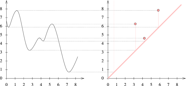
Figure 1. On the left, we see the graph of a function $f$ in  ${\mathbb{R}}^{2}$. On the right is the corresponding persistence diagram,  Dgm${}_{0}(f)$. Each point is drawn with multiplicity one. The birth at the point $(7,1)$ remains unpaired.

As $s$ increases from negative infinity, we label each new component with the positive critical value that introduces the component. We pair each negative critical value $s$ with the most recently discovered unpaired positive critical value representing the components joined at $s.$ This will lead to the diagram Dgm${}_{0}(f)$ as demonstrated in Figure 1. Consider one pair: a positive critical value that was introduced at time $s=s_{1}$ and a negative critical value that was introduced at time $s=s_{2}$, where $s_{1}<s_{2}$. This pair is represented in Dgm${}_{0}(f)$ as the point $(s_{1},s_{2}).$ The persistence of that pair is equal to the difference in function values: $s_{2}-s_{1}.$ In Figure 1, there are three pairs of points and one positive critical value that remains unmatched. This value represents an essential homology class. It would be paired if we were to consider the extended persistence diagram as presented in  [6].

2.3. Relationships between Diagrams

We now turn to looking at two functions. Two functions are called homotopic if there exists a continuous deformation of the first function into the second. We are interested in creating a homotopy between $f$ and $g$ in order to observe how the corresponding persistence diagram changes through time. More importantly, we use the homotopy when matching points in the persistence diagrams. Before proceeding, let us formally define a homotopy and give an example that we will use later.

Definition 2.1 (Homotopy).

We say that $f,g\colon{\mathbb{M}}\to{\mathbb{R}}$ are homotopic if there exists a continuous function $F\colon{\mathbb{M}}\times[0,1]\to{\mathbb{R}}$ such that $F(x,0)=f(x)$ and $F(x,1)=g(x)$, for all  $x\in{\mathbb{M}}$. We will denote the homotopy $F(x,t)$ by  $f_{t}(x)$.

Example 2.2 (The Straight Line Homotopy).

The straight line homotopy interpolates linearly from each point in the continuous function $f$ to the corresponding point in the continuous function  $g.$ We can write $f_{t}(x)=(1-t)\cdot f(x)+t\cdot g(x)$ for all $t\in[0,1]$ and all $x\in M$.

For $f,g\colon{\mathbb{M}}\to{\mathbb{R}}$, we have a diagram for each integer $p\in\{0,1,2\}$. Now, choose a value of $p$ and assume that we have a homotopy (not necessarily the straight line homotopy) from $g$ to  $f$. Choose $\tau$ time-steps of the homotopy, $0<t_{1}<\ldots<t_{\tau}=1.$ Let $t_{0}=0$, so that Dgm${}_{p}(f_{0})$ is the initial persistence diagram. At each time $t_{j}$, we have a persistence diagram Dgm${}_{p}(f_{t_{j}})$. Moreover, given Dgm${}_{p}(f_{t_{j}})$, we can compute Dgm${}_{p}(f_{t_{j+1}})$ in time linear in the number of simplices of the filtration by using a straight line homotopy between $f_{t_{j}}$ and $f_{t_{j+1}}$, as described in  [8]. In Section 5.2, we describe how to use information obtained from this computation in order to pair points in the persistence diagrams. Then, we stack the diagrams so that Dgm${}_{p}(f_{t})$ is drawn at height $t$ in ${\mathbb{R}}^{3}$ and connect the points in the diagrams by curves formed by the line segments connecting matched points in consecutive diagrams. The result is a piecewise linear path between points in Dgm${}_{p}(f_{0})$ and points in Dgm${}_{p}(f_{1})$. If we let the time difference between any two consecutive diagrams approach zero, the piecewise linear path becomes a set of continuous curves by the stability result for the straight line homotopy (see Section 3.4). Each curve that traces the path of an off-diagonal points through time is called a vine. The collection of vines is referred to as a vineyard  [8, 10]. We pair the endpoints of each vine to obtain a matching of the persistence points in Dgm${}_{p}(g)$ with the points in Dgm${}_{p}(f)$.

3. Matching Persistence Diagrams

To match the points in Dgm${}_{p}(g)$ and Dgm${}_{p}(f)$ without considering the homotopy, we look at methods of finding matchings on bipartite planar graphs. We begin this section with a few definitions. A matching is a bipartite graph $P=(A\cup B,E)$ where the vertex sets $A$ and $B$ are disjoint, the edges are between one vertex in $A$ and one vertex in $B$, and each vertex is incident on at most one edge. A matching is maximal if the addition of any edge would result in a graph that is no longer a matching. A matching is perfect if every vertex is incident upon exactly one edge. In other words, it is a matching where there does not exist an unmatched vertex.

We consider two different methods for measuring the distance between the persistence diagrams, Dgm${}_{p}(f)$ and Dgm${}_{p}(g)$. The goal is to match every point in $A=$Dgm${}_{p}(f)$ to a point in $B=$Dgm${}_{p}(g)$ in order to minimize the cost of the matching. One method for determining this cost is to consider the bipartite matching problem, where for every $a\in A$ and $b\in B$, the edge  $\{a,b\}$ has a cost $C(a,b)$. Then, the cost of a perfect matching is the sum (or the maximum) value of the edge costs. The cost for a matching that is not perfect is infinite. To resolve the issue where the number of off-diagonal points in both diagrams is not equal or the diagrams are dissimilar, we allow an off-diagonal point to be matched to a point on the line $y=x$. The use of the bottleneck and Wasserstein matchings for this purpose is presented in Chapter VIII of  [10]. As we will show, each of these methods entails some notion of stability for the persistence diagrams. That is, we can bound the bottleneck and Wasserstein distance between persistence diagrams by the distance between $f$ and  $g$, for some class of functions.

3.1. Two Cost Metrics

Consider the matching problem where we must match the elements of set $A\subseteq{\mathbb{R}}^{2}$ with elements of a second set $B\subseteq{\mathbb{R}}^{2}$, and where there is a cost associated with each pair $(a,b)\in A\times B$. We will define both the bottleneck and the Wasserstein costs of a matching. Later, we will use these distance metrics as the costs to find the bottleneck and the Wasserstein matchings. Let $C(a,b)$ be the $L_{\infty}$ distance between the points $a$ and $b$; that is, $C(a,b)=\max\{|a_{x}-b_{x}|,|a_{y}-b_{y}|\}.$

Definition 3.1 (Bottleneck Cost).

The bottleneck cost of a perfect matching $P$ is the maximum edge cost:

$$\max_{(a,b)\in P}C(a,b).$$

Definition 3.2 (Wasserstein Cost).

The degree $q$ Wasserstein Cost of a perfect matching is sum of the edge cost over all edges in the matching:

$$\left(\sum_{(a,b)\in P}{C(a,b)^{q}}\right)^{1/q}.$$

3.2. The Bottleneck Matching Criterion

The bottleneck matching minimizes the bottleneck cost of a matching over all perfect matchings of $A$ and  $B$:

$$W_{\infty}(A,B)=\min_{P}\max_{(a,b)\in G}C(a,b).$$

The use of the notation $W_{\infty}$ to denote the bottleneck distance will become clear in the next section.

If $|A|=|B|=n$, then a maximal matching can be found in $O(n^{5/2})$ using the Hopcroft-Karp algorithm  [15]. If we mimic the thresholding approach of the hungarian method  [16], then the bottleneck solution can be found in  $O(n^{5/2}\log n)$. Since $A$ and $B$ are sets of points in the plane, we can improve the computational complexity of determining the matching under the bottleneck distance. Efrat, Itai, and Katz developed a geometric improvement to the Hopcroft-Karp algorithm with a running time of $O(n^{1.5}\log^{2}n)$  [12].

3.3. The Wasserstein Matching Criterion

In the Wasserstein Matching, we seek to minimize the maximum degree $q$ Wasserstein cost over all perfect matchings:

$$W_{q}(A,B)=\min_{P}\left(\sum_{(a,b)\in M}{C(a,b)^{q}}\right)^{1/q}.$$

Although for small values of $q$, the bottleneck and the Wasserstein criteria may produce different matchings, if we take the limit as $q\to\infty$, we see that the Wasserstein criterion approaches the bottleneck criterion.

The Hungarian method computes the Wasserstein matching in $O(n^{4})$ computational complexity  [16]. In  [19], Vaidya maintains weighted Voronoi diagrams for an $O(n^{2.5}\log n)$ computation of this matching. Further improvements were made by Agarwal, Efrat, and Sharir  [1]. They utilize a data structure that improves the running time to $O(n^{2+\epsilon})$ for the min-weight Euclidean matching.

3.4. Stability Theorems

A distance metric (and corresponding matching) is stable if a small change in the input sets $A$ and $B$ produces a small change in the measured distance between the sets. The property of stability is not obvious and sometimes not true. If a matching is stable, however, we can use it to create a vineyard from a smooth homotopy.

Let $P_{\infty}$ be the matching obtained using the bottleneck criteria; that is, the matching $P_{\infty}$ is the matching that minimizes the bottleneck distance. Let $f,g$ be tame functions. This means that the homology groups of ${\mathbb{M}}_{s}^{f}$ and of ${\mathbb{M}}_{s}^{g}$ have finite rank for all $s.$ In addition, only a finite number of homology groups are realized as $H_{p}({\mathbb{M}}_{s}^{f})$ or $H_{p}({\mathbb{M}}_{s}^{g})$  [11]. The function difference $||f-g||_{\infty}$ is the maximum difference between the function values:

$$||f-g||_{\infty}=\sup_{x\in X}|f(x)-g(x)|.$$

The Stability Theorem for Tame Functions, which gives us that the bottleneck distance $W_{\infty}(\text{Dgm}_{p}(f),\text{Dgm}_{p}(g))$ is bounded above by $||f-g||_{\infty}$  [5]. The proof of this theorem presented in [8] uses the following result:

• Given $f_{t}(x)$, the straight line homotopy from $g$ to $f$, we know that there exists a perfect matching $P$ of the persistence diagrams for $f$ and $g$ such that the bottleneck cost of $P$ is upper bounded by the distance between $f$ and $g$:

  $$\max_{(a,b)\in P}C(a,b)\leq||f-g||_{\infty}.$$

We will explain how to obtain this matching $P$ in Section 5.3.

The Wasserstein distance is stable for Lipschitz functions with bounded degree $k$ total persistence. This is proven in  [7]. If we relax either of these two conditions, then the Wasserstein distance becomes unstable for two functions $f$ and $g$ where $||f-g||_{\infty}\leq\epsilon$ as $\epsilon$ approaches zero.

4. The Heat Equation

The heat equation is a mathematical description of the dispersion of heat through a region in space. We start with the initial reading (or a guess) of the temperature throughout an enclosed space, say an empty room. After infinite time and given no external changes, the temperature at each point in the space will converge to the average initial temperature.

4.1. Dispersing the Difference

Let the manifold ${\mathbb{M}}$ be a closed square subset of ${\mathbb{R}}^{2}$. Then, we can think of the functions $f,g\colon{\mathbb{M}}\to{\mathbb{R}}$ as surfaces in ${\mathbb{R}}^{3}$. Now, let $u_{0}$ be the difference $g-f$. If $u_{0}(x)=0$ for all $x\in M$, then we have $f=g$. Otherwise, define the average of a function as the integral divided by the area.

$$\text{avg}(f)=\frac{\int_{M}f(x)dx}{\text{area}({\mathbb{M}})}$$

and

$$\text{avg}(g)=\frac{\int_{M}g(x)dx}{\text{area}({\mathbb{M}})}.$$

Then, we can calculate the average value of $u_{0}$ over the domain ${\mathbb{M}}$ by subtraction:

$$\text{avg}(u_{0})=\text{avg}(g)-\text{avg}(f).$$

We apply the heat equation to $u_{0}$ and obtain $u(x,t)$ where $u(x,0)=u_{0}(x)$ and $\lim_{t\to\infty}{u(x,t)}=c$. For sake of simplicity, we will assume that the average of $u_{0}$ vanishes. If this is not the case, we can impose this condition by setting  $g=g-\text{avg}(u_{0})$.

Now, we can observe the difference $u$ disperse through time until $u$ becomes the zero function. Similarly, we know that $f(x)+u(x,t)$ will go from $g$ to $f$. Although the value of $u(x,t)$ approaches zero for all $x$ as $t$ increases

$$\lim_{t\to\infty}{u(x,t)}=0,$$

we will stop at a time $T$ when $u(x,T)\in(-\epsilon,+\epsilon)$ for all $x\in{\mathbb{M}}$ and for some $\epsilon>0$. Then, the function $f+u$ goes from $g$ to a function close to $f$. Furthermore, the manner in which the function $f+u$ changes is dictated by the heat equation.

4.2. The Continuous Heat Equation

Here, we describe the heat equation as it applies to a continuous function. For more details, please refer to  [2, 4]. In Section 4.3, we will modify these equations to approximate the solution in the discrete case and we introduce the heat equation homotopy.

Let $\{b_{1},b_{2}\}$ be an orthonormal basis for ${\mathbb{M}}$. The general form of the heat equation satisfies the following conditions:

(1) $$\frac{\partial u}{\partial t}(x,t)-\frac{\partial^{2}u}{\partial b_{1}^{2}}(x,t)-\frac{\partial^{2}u}{\partial b_{2}^{2}}(x,t)=0$$

and the initial condition:

(2) $$u(x,0)=g(x)-f(x),x\in{\mathbb{M}}.$$

If we can solve this partial differential equation (PDE), we obtain $u(x,t)$ defined for all $x\in{\mathbb{M}}$ and $t\geq 0.$ Typically, the heat equation has the additional constraint that $u(x,t)$ is constant with respect to $t$ for all $x\in\partial{\mathbb{M}}$. However, we are interested in the case where $u(x,t)$ is heat conserving. That is, we would like avg$(u_{t_{1}})=$avg$(u_{t_{2}})$ for all $t_{1}$, $t_{2}$. As we will show, in order to obtain this goal, the values on the boundary will reflect the values interior to the boundary.

The equation in (1) describes how the temperature changes with respect to time and space. We note that if we impose the condition $\frac{\partial u}{\partial t}(x,t)=0$, then the heat equation will not change with respect to time, and Equation  (1) becomes Laplace’s equation, $\Delta u(x,t)=0$. This is known as the steady-state heat equation and will have a unique solution. The iterative methods that we look at in Section 4.3 aim at finding an approximation of $u(x,t)$ for this problem. The final solution will be constant with respect to time, and so we say it is approaching the steady-state. We are interested in following the behavior of heat equation as it approaches the solution to the steady-state heat equation.

4.3. The Discrete Heat Equation Homotopy

Solving a partial differential equation is not a simple task. Thus, we must defer to numerical methods to estimate this solution, which require spatial and temporal discretization  [4]. In the following computations, we use a regular grid decomposition of ${\mathbb{M}}=[0,1]^{2}$, writing $x_{i}=(i-1)h$ and $y_{j}=(j-1)h$, where $h=1/(n-1)$ for some fixed integer $n\geq 2$. In the next section, we explain how to apply the heat equation on different topologies.

The first step in creating the heat equation homotopy $f_{t}(x)$ is to compute $u_{t}(x)=u(x,t)$ over the discretized domain. There are three issues that can arise when using the continuous formulation of the heat equation described in Section 4.2.

1. We need to solve the partial differential equation presented in Equations (1) and (2).

2. The partial derivative $\frac{\partial^{2}u_{t}}{\partial b_{i}^{2}}(x)$ for $b_{i}$ is not well defined over a discrete domain.

3. The solution $u(x,t)$ is defined for all non-negative $t,$ but a homotopy must to be defined for $t\in[0,1].$

In order to resolve these issues, we apply temporal and spatial discretization as well as scaling. The goal is to obtain a homotopy $f_{t}(x)$ from $g$ to $f$ using the heat equation solution $u(x,t).$ Below, we describe one such resolution; note, however, that other approaches may be taken.

4.3.1. Mathematical Description of the Heat Equation

Let us recall the steady-state heat equation over ${\mathbb{R}}^{2}$:

(3) $$\frac{\partial^{2}u}{\partial b_{1}^{2}}(x,t)+\frac{\partial^{2}u}{\partial b_{2}^{2}}(x,t)=0.$$

In this equation, we are using $\{b_{1},b_{2}\}$ as the standard basis vectors for ${\mathbb{R}}^{2}$. At each mesh point $x=(i,j)$, we employ the Taylor polynomial in the variable $b_{1}$ to obtain an approximation of the second derivative with respect to $b_{1}$:

(4) $$\frac{\partial^{2}u}{\partial b_{1}^{2}}u((i,j),t)=\frac{u(({i+1},j),t)-2u((i,j),t)+u(({i-1},j),t)}{h^{2}},$$

where $h$ is the spatial step size. Similarly, we also have an approximation for the second derivative with respect to $b_{2}$:

(5) $$\frac{\partial^{2}u}{\partial b_{2}^{2}}u((i,j),t)=\frac{u((i,{j+1}),t)-2u((i,j),t)+u((i,{j-1}),t)}{h^{2}}.$$

To simplify notation, we will now use $x_{i,j}$ to denote $(i,j)$. If we plug (4) and (5) into (3), then we obtain the following equation:

(6) $$4u(x_{i,j},t)-u(x_{i+1,j},t)-u(x_{i-1,j},t)-u(x_{i,j+1},t)-u(x_{i,j-1},t)=0$$

Thus, the approximation to the heat equation is made by looking at local neighborhoods for each point $x_{i,j}$. Figure 2 highlights the four neighbors of the mesh needed to compute an approximation to the heat equation.

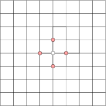
Figure 2. In the center, we have the white dot representing the mesh at position $x=(i,j)$. The mesh points highlighted in pink are those whose values contribute to the estimate of the heat equation at $x$.

The neighborhood of a point, Nhd$(i,j)$, is defined to be the set of local neighbors of the point $x_{i,j}$.

(7) $$\text{Nhd}(i,j)=\{(i,j\pm 1),(i\pm 1,j)\}$$

We have $n^{2}$ equations of the form presented in (6), one for each point in the $n\times n$ mesh. We relabel the mesh points in column-major order in order to use one index instead of two: $v_{\{(j-1)n+i\}}:=u(x_{i,j},t)$. Then, we may express the $n^{2}$ linear equations in matrix-vector form,  $Av=0$.

4.3.2. An Iterative Algorithm for Linear Systems of Equations

As we have shown above, solving the discrete heat equation finds a solution $v$ to the linear system of equations $Av=0$. Above, we have described how to construct the matrix $A$, as it is the coefficient matrix for the system of linear equations. In the above description, $A$ is equal to $L_{n}$, the Poisson matrix of order $n$. We note here that this matrix is $n^{2}\times n^{2}$. We can write $L_{n}=D-N$, where $D$ is the diagonal matrix $4\cdot I$ and $N$ is a matrix with $0$’s on the diagonal and with only $1$ as the non-zero entries of the matrix. Sometimes we refer to $D$ as the valency matrix, since it expresses the degree of each mesh point. The matrix $N$ is symmetric and we call it the neighborhood matrix since the non-zero entries in row $i$ correspond to the neighbors of the mesh point $v_{i}$  [3]. That is, $N(i,j)=1$ iff $v_{i}$ and $v_{j}$ are adjacent.

The iterative algorithm can be defined by these matrices. We want a solution of the form $Av=0$, which means $(D-N)v=0$. We can re-write this so that $Dv=Nv$. And, the iterative algorithm can immediately be seen:

(8) $$v_{\text{new}}=(D^{-1}N)v.$$

In the original formulation, this translates to:

$$u_{t+1}(x)=\frac{1}{4}\sum_{y\in\text{Nhd}(x)}u_{t}(x),$$

where the neighborhood Nhd$(x)$ is the neighborhood of $x$ defined by Equation (7). This iterative method is known as Jacobi iteration.

4.3.3. Creating the Homotopy

We continue the process of obtaining $u_{t+1}$ from $u_{t}$ until we have reached a halting point, where $|u_{t+1}(x)-u_{t}(x)|\leq\epsilon$ for all $x\in{\mathbb{M}}$ and for some predetermined value of $\epsilon$. We will let $T$ be the maximum time computed in the iterative method. Thus, we have a function  $u:{\mathbb{M}}\times[0,T]\to{\mathbb{R}}.$ We reparameterize $u(x,t)$ with respect to $t$ in order to obtain $\tilde{u}(x,t)=u(x,{t}\cdot{T})$ defined over the domain ${\mathbb{M}}\times[0,1].$ Then, the heat equation homotopy $f_{t}$ can be defined by the equation:

(9) $$f_{t}(x)=f(x)+\tilde{u}(x,t).$$

Notice that $f_{0}(x)=g(x)$ and $f_{1}(x)\approx f(x)$ with $T$ sufficiently large since

$$\lim_{T\to\infty}f_{1}(x)=\lim_{T\to\infty}f(x)+u(x,T)=f(x).$$

By using this homotopy, the initial difference between $f$ and $g$ disperses. Although $\tilde{u}(x,t)$ approaches a constant function as $t$ approaches $T$, interesting things can happen along the way. For example, critical values can be created.

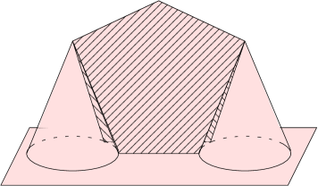
Figure 3. The function used in Example 4.1.

Example 4.1 (Mountain and Bridge).

Suppose we have two cones connected by two pentagons as shown in Figure 3. We will call this surface $S$. Now, consider the height $h\colon{\mathbb{R}}^{2}\to{\mathbb{R}}$ defined to be the height of the surface at $(x,y)$ below $S$ and zero elsewhere. We assume that the base of the cones and the pentagons is in the $xy$-plane. There is one dimension one critical value, the pinnacle of the pentagons. If we apply the heat equation to this surface, there will soon be at least three dimension zero critical values: one corresponding to the original critical value and two from the cone tips.

4.4. Considering Different Topologies

Here, we consider implementing different topologies for the square domain. Each mesh element has four neighbors, corresponding to above, below, left, and right. The topologies are determined by which vertices we define to be neighbors. We consider four topologies: the square, the torus, the Klein bottle, and the sphere. The square topology, used when describing the iterative heat equation, is the most basic.

Definition 4.2 (Square Topology).

The neighborhood of $(i,j)$ is:

$$Nhd(i,j)=\{(i,j\pm~{}1),(i\pm 1,j)\},$$

provided that these elements are within the domain.

Each vertex can have two, three, or four neighbors, resulting in a system of equations that does not conserve heat. Let $V$ be the set of vertices in ${\mathbb{M}}$, and define the total heat to be the sum of the heat over the entire domain:  $\sum_{x\in V}u(x).$ Then, the total heat is not preserved between iterations. To fix this, let $x$ be its own neighbor for every neighbor that $x$ is missing. Hence, each $x\in V$ is the neighbor of four other vertices and has four neighbors itself. For the second step, we have

$$\sum_{x\in V}u(x,t+1)=\sum_{x\in V}\frac{4u(x,t)}{4}=\sum_{x\in V}u(x,t).$$

The four edges of the square create the boundary on the square topology. If we identify the boundary edges in pairs, we can then create a surface without boundary. One way to do this is to create a torus from the square. Formally, we define the torus topology as follows:

Definition 4.3 (Torus Topology).

Given an $n\times n$ mesh, the neighborhood of $(i,j)$ is:

$$Nhd(i,j)=\{(i,j\pm_{n}1),(i\pm_{n}1,j)\},$$

where addition and subtraction are calculated modulo $n$.

The torus topology can also be described by Figure 4.

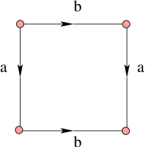
Figure 4. The torus is the quotient of the unit square by gluing together opposite sides as prescribed by their orientation.

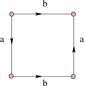
(a) The Klein bottle

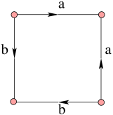
(b) The sphere

Figure 5. The figures above illustrate how the boundaries of the square are glued to obtain the Klein bottle and the sphere.

By gluing the two $a$ edges together and the two $b$ edges together, we obtain a manifold without boundary. In this manifold, each vertex $v$ is the neighbor of four other vertices, and has four neighbors that contribute to the new value for that vertex. Similarly, we can define the Klein Bottle and the Spherical topologies as depicted in Figure 5.

4.5. Convergence

When using iterative algorithms, we worry about how long finding the solution (or something close to the solution) will take. In this section, we discuss one metric that measures the convergence of iterative algorithms.

If $x^{(k)}=u(x,t_{k})$ is the solution at stage $k$, then the solution at stage $k+1$ is

$$x^{k+1}=\frac{1}{4}Nx^{(k)}.$$

We now see that

(10) $$Dx^{(k+1)}=Nx^{(k)}$$

and for the solution $x^{\infty}$:

(11) $$Dx^{\infty}=Nx^{\infty}.$$

If we subtract (10) from (11), then we obtain

$$DE_{k+1}=NE_{k},$$

where $E_{k}=x^{\infty}-x^{k}$ is the error of the $k^{th}$ estimate $x^{(k)}$. Hence,

$$E_{k+1}=D^{-1}NE_{k}=(D^{-1}N)^{k+1}E_{0}.$$

The action of $M=D^{-1}N$ on the initial error determines whether the error of the solution $x$ will increase or decrease. Now, if $M$ has $n^{2}$ non-degenerate eigenvalues and $n^{2}$ linearly independent eigenvectors, we can write $M=V\Sigma V^{-1}$, where $\Sigma$ is the diagonal matrix of eigenvalues. Since $M^{k}=V\Sigma^{k}V^{-1}$, we use the spectral norm of the matrix $M$ to determine if the error is compounding or decreasing. The spectral norm, $\rho$, of a matrix the largest absolute eigenvalue of that matrix. If $\rho<1$, then the iterative algorithm converges. If $\rho>1$, then the iterative algorithm does not converge. For example, if we are using Jacobi iteration as described in Section 4.3.2, then $\rho$ is very close to one, and thus convergence is very slow  [14]. Although this is undesirable behavior for finding a solution to the heat equation, for our purposes, it allows us to more closely examine the behavior of the heat equation.

5. Vineyards of the Heat Equation Homotopy

In Section 2.3, we defined homotopy and stated that we can stack the persistence diagrams associated with the homotopy to create a vineyard. In this section, we estimate the underlying vineyard for the heat equation homotopy by monitoring the transpositions in the filter.

5.1. Turning a Mesh into a Filter

We begin with an $n\times n$ matrix of values. Although the heat equation computes neighbors based on a grid, we will be computing persistence using simplicial complexes. Thus, we triangulate the domain by adding in horizontal, vertical and diagonal edges, as well as the triangles formed by the voids.

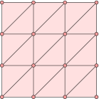
Figure 6. The triangulation of a $4\times 4$ grid.

An $n\times n$ mesh gives us $n^{2}$ vertices, $(n-1)(3n-1)$ edges, and $2(n-1)^{2}$ faces. In Figure 6, we see the triangulation of a four-by-four mesh. Each simplex $\sigma$ is defined by the vertices that create it. In addition, the value of a simplex, $f(\sigma)$, is the maximum function value of those vertices. Now, we order the simplices by the following two rules:

1. If $f(\sigma_{1})<f(\sigma_{2})$. then $\sigma_{1}$ appears before simplex $\sigma_{2}$.

2. If $\tau$ is a subsimplex of $\sigma$, denoted $\tau\leq\sigma$, then simplex $\tau$ appears before simplex $\sigma$.

We observe here that the second rule does not contradict the first, because $f(\tau)\leq f(\sigma)$ whenever $\tau$ is a face of $\sigma$. The resulting ordering of the simplices is called a filter. The two rules imply that every initial subsequence of the filter defines a subcomplex of the mesh. Growing this initial subsequence until it equals the entire filter gives a sequence of simplicial complexes called the induced filtration. As with any sorting algorithm, to create a filter of $m$ simplices will take $O(m\log m)$ time.

5.2. Computing Vines

Recall the heat equation homotopy from Equation (9),

$$f_{t}=f(x)+\tilde{u}(x,t),$$

which is defined over a finite number of time-steps: $0,t_{1},t_{2},\ldots,t_{T}=1$. Create a filtration for $f_{0}(x)$ as prescribed above. We use the filtration to compute the persistence diagrams, just as we used the sublevel sets in Section 2.2. We progress from one complex in the filtration to another by adding one simplex. The addition of this simplex can be the birth of a new homology class or the death of an existing homology class. After we have iterated through the entire filter, we have completed the computation of the persistence diagrams for time  $0$.

To compute Dgm${}_{p}(f_{t_{1}})$, we could repeat the same process. However, if we use Dgm${}_{p}(f_{t_{0}})$, we can compute the new diagram in linear time and we can match points in the two diagrams  [8].

5.2.1. Transpositions

Suppose we have two filters on $m$ simplices, such that the filters are identical except that two adjacent simplices have swapped order. Then, we can write the first filter:

$$F1:\sigma_{1},\sigma_{2},\ldots,\sigma_{i},\sigma_{i+1},\ldots,\sigma_{m}$$

and the second filter:

$$F2:\sigma_{1},\sigma_{2},\ldots,\sigma_{i+1},\sigma_{i},\ldots,\sigma_{m}.$$

If we have the persistence diagram for the filter $F1$, then we can compute the persistence diagram for the the filter $F2$ by performing one transposition. A transposition updates the persistence diagram by changing the pairings of two consecutive simplices, if necessary. In the case that $\text{dim}(\sigma_{i})\neq\text{dim}(\sigma_{i+1})$, the transposition does not affect the pairs in the persistence diagram. Thus, only the transposition of simplices with the same number of vertices can result in a pairing swap. One transposition can swap the births and deaths of at most two points in the persistence diagram.

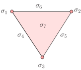
Figure 7. The filter of a simplicial complex is an ordering on the vertices, edges, and faces. The simplices are originally ordered $\sigma_{1}$ through  $\sigma_{7}$. Swapping $\sigma_{1}$ and $\sigma_{2}$ results in a pairing swap of type  $1$. Swapping $\sigma_{4}$ and $\sigma_{5}$ results in a pairing swap of type  $2$. Swapping $\sigma_{5}$ and $\sigma_{6}$ results in a pairing swap of type  $3$.

We must distinguish between nested and unnested persistence pairings. We say that two persistence points, $(b_{1},d_{1})$ and $(b_{2},d_{2})$, are nested if the birth at $b_{2}$ and the death at $d_{2}$ occur after $b_{1}$ and before $d_{2}$. Assuming all events happen at distinct moments of time, this is equivalent to  $b_{1}<b_{2}<d_{2}<d_{1}$. If we transpose $\sigma_{i}$ and $\sigma_{i+1}$, then the three types of pair-swapping transpositions are:

1. The births of two nested pairs are transposed. In this case, $\sigma_{i}$ is associated with $b_{1}$ in Dgm${}_{p}(F1)$, and with $b_{2}$ in Dgm${}_{p}(F2)$.

2. The deaths of two nested pairs are transposed. In this case, $\sigma_{i}$ is associated with $d_{2}$ in Dgm${}_{p}(F1)$, and with $d_{1}$ in Dgm${}_{p}(F2)$.

3. The birth of one pair and the death of another, unnested, pair are transposed. In this case, the addition of $\sigma_{i}$ to the filtration created a death in Dgm${}_{p}(F1)$, but a birth in Dgm${}_{p}(F2)$.

Figure 7 illustrates the three types of transpositions that can be made. Although pair swaps of types $1$ and $2$ involve two persistence points in the same diagram, pair swaps of type $3$ involve persistence points in diagrams of two consecutive dimensions. In each of the cases, the transposition results in a swap only if changing the order in which the simplices are added changes the persistence pairing that is made. For a complete algorithm to compute the transpositions, please refer to  [8].

From these transpositions, we can create the matching referred to in Stability Result of the Straight Line Homotopy of 3.4. Suppose the transposition of $\sigma_{i}$ and of $\sigma_{i+1}$ resulted in a pairing swap. Then, every persistence point is paired with itself in the matching, except for $(b_{1},d_{1})$ and  $(b_{2},d_{2})$, whose pairings are swapped.

5.2.2. Sweep Algorithm

Changing one filtration into another may require more than one transposition. In order to compute the persistence diagram, we first create a topological arrangement and then use a sweep algorithm.

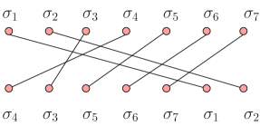
Figure 8. We create a topological arrangement by connecting drawing a line between the vertices that represent the same simplex. By doing this, we find a finite number of crossings. Each crossing represents one transposition in the filter.

In the Cartesian plane, write the filtration of $f_{t_{j}}$ horizontally. Below that, write the filtration of $f_{t_{j+1}}$ using the same simplex names. Then, we connect like simplices with a single curve (does not need to be straight). An example of this process is given in Figure 8. After this arrangement has been created, an ordering on the transpositions can be found by topologically sweeping the arrangement, as presented in [9].

We compute Dgm${}_{p}(f_{t_{j+1}})$ and keep track of the matching by progressing one transposition at a time in the order dictated by the sweep algorithm.

5.3. Measuring Distance between Persistence Diagrams

Now, we assume that there exists a homotopy between functions $f$ and $g.$ Then, we have a vineyard that connects each point $a$ in $A=$Dgm${}_{p}(f)$ with a point $b$ in $B=$Dgm${}_{p}(g).$ We will use this pairing as our matching and define a distance metric for it.

Assume $a$ and $b$ are connected by the vine $s:[0,1]\to{\mathbb{R}}^{3},$ as described in Section 5.2. Since the vine was created from a homotopy, we will use the index $t$ to emphasize that $s(t)$ is a persistence point for the function $f_{t}(x).$ The velocity of the vine $\frac{\partial s}{\partial t}$ will be integrated on $[0,1]$ in order to measure the distance traveled between $a$ and $b:$

$$D_{s}=\int_{0}^{1}\frac{\partial s(t)}{\partial t}\,dt.$$

In order to obtain a distance between persistence diagrams we sum these distances over all vines in the vineyard $V$:

(12) $$D_{fg}=\sum_{s\in V}D_{s}.$$

If $s(t)$ is only defined for a discrete set of times $t_{i}$ with $0\leq i\leq T$, then we obtain an alternate definition for  $D_{fg}$:

(13) $$D_{fg}=\sum_{s\in V}\sum_{i\in(0,T]}||s(t_{i})-s(t_{i-1})||_{\infty}.$$

When a point $a\in A$ enters the diagonal at $t<1,$ we pair $a$ with the corresponding diagonal point, since the diagonal points can only occur as endpoints of a vine by definition of vine in Section 5.2. Then, we only measure the distance over the interval in which the vine is defined, $[0,t).$ Symmetrically, we can have a diagonal point in $A$ paired with an off-diagonal point in $B$.

We are interested in understanding how this distance metric compares with the bottleneck and Wasserstein distances, as well as to understand the properties of this distance metric and homotopy matching.

6. An Example

In this section, we present the results from one example. Although the results from one example cannot be generalized, we are able to capture the different behaviors of the homotopy under the four topologies (square, sphere, torus, and Klein bottle). In the subsequent examples, ${\mathbb{M}}$ is a square closed region of ${\mathbb{R}}^{2}.$ The functions $f$ and $g$ are approximated by a $101\times 101$ mesh. We obtain the function values from two gray-scale images of a bird and a flower respectively, as shown in Figure 9. The difference $u_{0}=g-f$ is computed. From here, we will find a homotopy from $u_{0}$ to the zero function. We note that this homotopy differs from the one previously defined, since we do not add $f$ to the heat equation solution. In practice, we found that this homotopy more clearly displays the behavior of the heat equation.

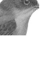
(a) Bird

(b) Flower

(c) Difference

Figure 9. The homotopy acts on the difference between the image of the bird and the image of the flower. The grayscale values of the image of the difference represent the values of the height function　 $u_{0}$. In the images, the dark pixels correspond to the low values and the light pixels correspond to the high values.

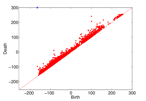
Figure 10. The persistence diagram of the difference function. This is the diagram at Step $0$ of the heat equation under the square topology. The possible values are the integers in  $[-255,255]$. The blue star drawn at height $300$ represents the essential homology class.

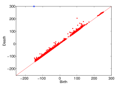
(a) Step 1

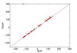
(b) Step 10

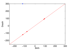
(c) Step 100

Figure 11. Persistence diagrams for the heat equation using square topology.

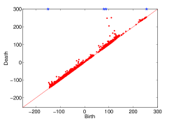
(a) Step 1

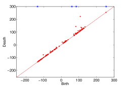
(b) Step 10

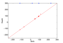
(c) Step 100

Figure 12. Persistence diagrams for the heat equation using torus topology.

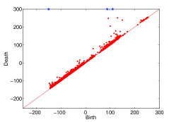
(a) Step 1

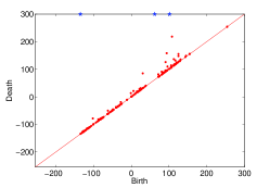
(b) Step 10

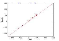
(c) Step 100

Figure 13. Persistence diagrams for the heat equation using Klein bottle topology.

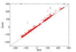
(a) Step 1

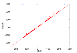
(b) Step 10

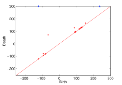
(c) Step 100

Figure 14. Persistence diagrams for the heat equation using spherical topology.

In Figures 10-14, we see several stages of the heat equation homotopy using various topologies of the square. The persistence diagrams shown are combined diagrams for all dimensions.

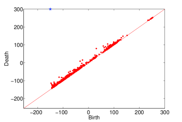
(a) Klein Bottle, Dimension 0

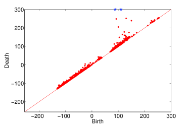
(b) Klein Bottle, Dimension 1

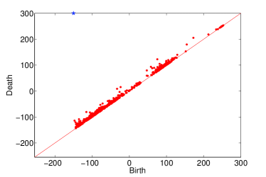
(c) Sphere, Dimension 0

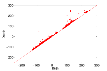
(d) Sphere, Dimension 1

Figure 15. In these figures, we separate the persistence diagrams from step one of the homotopy using the Klein bottle and the sphere topologies. The diagrams for combined dimensions are Figure 13(a) and Figure 14(a).

In Figure 15, we look at the diagram for the first step of the homotopy, separated for dimensions $p=0$ and $p=1$, under the Klein bottle and sphere topologies. We note that the points with the highest persistence appear in the dimension one persistence diagram. This is a property that remains true as the homotopy progresses.

6.1. Analyzing Different Topologies

Figure 16. A square with a high-valued (light-colored) region on the boundary.

In the topologies without a boundary (torus, Klein bottle, and sphere), a new feature is created with a relatively high persistence. For example, if we start with a triangular region of high values against a border, as in Figure 16, then there exists a $1$-cycle in the sublevel sets. Note, however, that there is not a $1-$cycle in any sublevel set of the square topology. Since we have created the four different topologies by gluing the edges of the square together in various ways, different behaviors along these edges can be expected. We keep this difference in mind as we continue to look for commonalities and other differences caused by the adopted topology.

The persistence diagrams for the torus and the Klein bottle topologies behave similarly. In most of the graphs in this section, the curves of the torus and the Klein bottle are usually parallel. This is an indication that orientability has little effect on the heat equation homotopy. This does not come as a not a surprise, as we did not use the orientation when computing the heat equation.

6.2. Duration of Vines

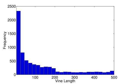
Figure 17. The distribution of the length of vines in the vineyard for Dgm${}_{0}(u_{t})$ under the square topology.

Table 1. Vine Length Statistics for Dgm${}_{0}(u_{t})$

	mean	median	mode	s.d.
square	63.2	15	6	132.8
sphere	69.4	25	6	143.8
torus	79.8	26	500	105.1
Klein	72.5	21	500	101.4

Table 2. Vine Length Statistics for Dgm${}_{1}(u_{t})$

	mean	median	mode	s.d.
square	119.6	65	6	97.7
sphere	122.5	56	6	94.2
torus	122.5	70	6	137.1
Klein	126.2	58	6	151.3

In Figure 17, we see the distribution of the vine lengths in the vineyard Dgm${}_{0}(u_{t})$. The histogram is skewed right, since the mean is greater than the median. Table 1 confirms this observation. The same pattern is in fact observed under different topologies. When comparing the vine lengths of any two topologies, the Kolmogorov-Smirnov test for statistical difference with $\alpha=.05$ fails to reject the null hypothesis that the distributions are the same. On the other hand, if we remove the short-lived vines, then we start to see that comparing the Klein bottle and sphere topologies results in the rejection of the null hypothesis. However, this is not a strong enough indication that these distributions are different. The details of this statistical method are out of the scope of this paper, but can be found in  [17].

From these observations we can conclude that all topologies display a similar distribution of the length of vines, with many of the vines being short-lived. In addition, under the torus and Klein bottle topologies, a large number of vines span the entire vineyard.

6.3. Monitoring Total Persistence

The degree $q$ total persistence is the sum of the $q^{th}$ powers of persistence over all points in the persistence diagram.

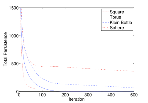
Figure 18. Total persistence of degree one.

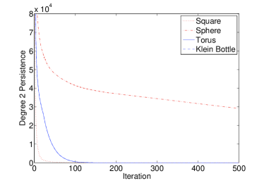
(a) Degree 2

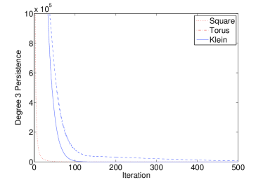
(b) Degree 3

Figure 19. The declining total persistence of degrees two and three. In the graph for the total persistence of degree three, we omit the sphere topology. Relative to the other topologies, the values were very high.

In Figure 18, we have the graph of the degree one total persistence versus the iteration. Although the total persistence rapidly deteriorates initially, the decay slows down around iteration $100$. - - We notice here that the Klein bottle and the torus have an end behavior different than that of the sphere and the square, in that we do not see the total persistence approaching zero after $500$ steps of the heat equation. - In these figures, the sphere behaves radically different than the other three topologies.

6.4. Mean Absolute Change

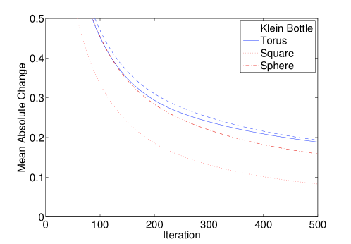
Figure 20. The mean absolute change between steps of the heat equation homotopy.

Figure 20 shows that the mean absolute value of the change between steps of the homotopy decreases rapidly at first, then slowly. Recall that the values of the mesh points range from $-255$ to $255$. At the first step, the mean absolute change is between $10$ and $15$ (not shown in Figure 20), which is only a $2\%-3\%$ initial change. The value, however, remains above $0.1$ in all cases except for the square topology. Given the nature of the heat equation, we expect the values to decrease with respect to time. The small values for mean absolute change are in part due to the initial values of $u_{0}$. The values of one vertex does not differ by a large amount from the values of its neighbors. We know that the iterative method chosen is slow to converge; however, this graph allows us to gauge how little change is occurring at each step of the homotopy.

6.5. Counting Transpositions

The total number transpositions between steps of the heat equation versus time is shown in Figure 21(a). All four topologies follow a decreasing pattern that levels off, with the Klein bottle and the torus behaving distinctively different from the square and the sphere.

We remark on several notable observations from these diagrams. The total number of transpositions is still significant when the heat equation algorithm reaches the halting condition. At the last step, the square topology makes over 400,000 total transpositions. The other three topologies make even more transpositions.

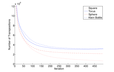
(a) Total

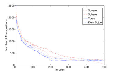
(b) Type 1 Pair Swap

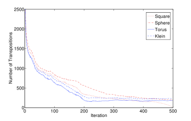
(c) Type 2 Pair Swap

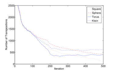
(d) Type 3 Pair Swap

Figure 21. The number of transpositions between steps of the heat equation homotopy. The top left shows the total number of transpositions and the remaining three figures are restricted to the three types of transpositions that result in pairing swaps.

In Figure 21 (b),(c), and (d) to see a different pattern for the number of the switches resulting from the transpositions. Under the square topology, the number of pair swaps of types 1, 2, and 3 is down to the double digits after $500$ iterations of the heat equation. We notice that Figures (b) and (c) are almost identical. This is not a surprising observation, since pairing swaps 1 and 2 (described in Section 5.2.1) are symmetric cases of two births of the same dimension or two deaths of the same dimension being transposed, resulting in a pair swap in the diagram.

Three other patterns are worth noting in the graphs of Figure 21. First, we see that the number of transpositions (of all kinds) rapidly decreases until iteration  $25$. At this point, the four topologies show different behaviors. Second, after iteration  $200$, the torus and the Klein bottle topologies have both leveled off to a constant function. Finally, we notice that adding graphs (b), (c), and (d) does not result in a graph that looks like (a). Thus, a significant number of the transpositions made are those that do not result in a pairing swap. Proportionally, this occurs more often in the torus and Klein bottle topologies than in the square and the sphere topologies.

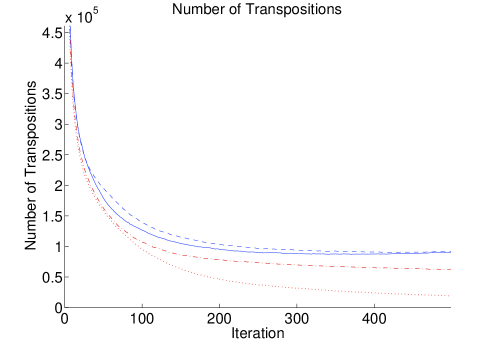
Figure 22. The number of transpositions between vertices versus the iteration of the heat equation.

In Figure 22, we restrict our counts to the number transpositions of vertices only. The values at the vertices dictates the values of the edges and the faces. The pattern that this graph follows is similar to Figure 21(a), the graph for the number of transpositions generated from all of the simplices Thus, is seems that the behavior of the vertex-vertex transpositions is proportional to the behavior of simplex-simplex transpositions.

7. Conclusion

The objective of this project was to find a new way of measuring the distance between two functions. We develop a homotopy of functions based on the heat equation and investigated the behavior of the vineyard resulting from this homotopy. We computed this homotopy using four topologies, and found some trends that differed from our expectation. For example, the heat equation on elliptic surfaces is known to converge more quickly than in Euclidean space. Yet, we found the behavior of the sphere topology to contradict this fact. We believe that this contradiction arises from the discretization of the sphere.

We began an investigation of the behavior of the heat equation homotopy; however, many directions still remain for where we can continue. We would like to explore if the observations made in Section 6 were specific to initial function $u_{0}$, or if we are observing behaviors that arise from the topologies used in the heat equation. Moreover, we would like to formally compare the matching we obtain with the bottleneck and Wasserstein matchings.

References

- [1] Agarwal, P. K., Efrat, A., and Sharir, M. Vertical decomposition of shallow levels in 3-dimensional arrangements and its applications. In SCG ’95: Proceedings of the Eleventh Annual Symposium on Computational Geometry (New York, NY, USA, 1995), ACM, pp. 39–50.
- [2] Alt, H. W. Analysis iii. Online., 2007. Lecture Winter Semester 2001/2002 at the Institute of Applied Mathematics, University of Bonn.
- [3] Babić, D., Klein, D., Lukovits, I., Nikoli, S., and Trinajsti, N. Resistance-distance matrix: A computational algorithm and its application. International Journal of Quantum Chemistry 90, 1 (2001), 166–176.
- [4] Burden, R. L., and Faires, J. D. Numerical Analysis, 8 ed. Thompson, 2005.
- [5] Cohen-Steiner, D., Edelsbrunner, H., and Harer, J. Stability of persistence diagrams. Discrete and Computational Geometry 37, 1 (2007), 103–120.
- [6] Cohen-Steiner, D., Edelsbrunner, H., and Harer, J. Extending persistence using Poincare and Lefschetz duality. Foundations of Computational Mathematics 9, 1 (2009), 79–103.
- [7] Cohen-Steiner, D., Edelsbrunner, H., Harer, J., and Mileyko, Y. Lipschitz functions have -stable persistence. Foundations of Computational Mathematics. To appear.
- [8] Cohen-Steiner, D., Edelsbrunner, H., and Morozov, D. Vines and vineyards by updating persistence in linear time. In SCG ’06: Proceedings of the twenty-second annual symposium on Computational geometry (New York, NY, USA, 2006), ACM, pp. 119–126.
- [9] Edelsbrunner, H., and Guibas, L. J. Topologically sweeping an arrangement. Journal of Computer and Systems Sciences 42 (1991), 249–251.
- [10] Edelsbrunner, H., and Harer, J. Computational Topology. An Introduction. American Mathematical Society, Providence, RI, USA. To be published in 2009.
- [11] Edelsbrunner, H., and Harer, J. Persistent homology–a survey. In A survey on Discrete and Computational Geometry: Twenty Years Later (2006), AMS, pp. 257–282.
- [12] Efrat, A., Itai, A., and Katz, M. J. Geometry helps in bottleneck matching and related problems. Algorithmica 31, 1 (2001), 1–28.
- [13] Hatcher, A. Algebraic Topology. Cambridge UP, 2002. Electronic Version.
- [14] Hockney, R., and Eastwood, J. Computer simulation using particles. Institute of Physics Publishing, 1988.
- [15] Hopcroft, J. E., and Karp, R. M. An n algorithm for maximum matchings in bipartite graphs. SIAM J. Comput. 2, 4 (1973), 225–231.
- [16] Kuhn, H. W. The hungarian method for the assignment problem. Naval Research Logistics Quarterly 2 (1955), 83–97.
- [17] Massey, Jr, F. J. The Kolmogorov-Smirnov Test for Goodness of Fit. Journal of the American Statistical Association (1951), 68–78.
- [18] Stewart, J. Calculus: Early Transcendentals, fourth ed. Brooks/Cole Publishing Company, 1999.
- [19] Vaidya, P. Geometry helps in matching. SIAM J. Comput. 18, 6 (1989), 1201–1225.