On closed cosmological models that satisfy the strong energy condition but do not recollapse

Abstract

We show the existence of a rather general class of closed cosmological models of Bianchi type IX that do not exhibit recollapse but expand for all times. This is despite the fact that these models satisfy the strong energy condition by a wide margin.

In relativistic cosmology, the trichotomy of the Friedmann-Robertson-Walker (FRW) models is of prime importance. The spatial geometry determines the evolution of the cosmological model: In the hyperboloidal ($k={-1}$) or the spatially flat ($k=0$) case, the universe exhibits an initial singularity (‘big bang’), and from that ‘moment’ on, the universe is forever expanding. In the case of a closed cosmological model ($k={+1}$) we observe a fundamentally different behavior: “[…] the dynamical equations of general relativity show that the spatially closed 3-sphere universe will exist for only a finite span of time. […] at a finite time after the big bang, the universe will achieve a maximum size […], and then will begin to recontract. […] a finite time after recontraction begins, a ‘big crunch’ will occur.” The quotation is taken from Wald:1984 . The recollapse of closed FRW cosmologies holds because the strong energy condition is imposed on the matter (which is assumed to be a perfect fluid), i.e., $\rho+3p\geq 0$, where $\rho$ is the energy density and $p$ the pressure.

On this basis it would be tempting to view the recollapse of the spatially closed FRW cosmologies satisfying the strong energy condition as a paradigm for models with less symmetries. That this belief is erroneous has been demonstrated in Barrow/Galloway/Tipler:1986 . At least in the case of cosmological models of Bianchi type IX, into which the closed FRW models are naturally embedded, there exists a rigorous result by Lin and Wald Lin/Wald:1989 : Assuming the dominant energy condition, i.e., $|p_{i}|\leq\rho$ for the anisotropic pressures $p_{1}$, $p_{2}$, $p_{3}$, and non-negative average principal pressure $p$, i.e., $3p=(p_{1}+p_{2}+p_{3})\geq 0$, then the ‘closed-universe-recollapse conjecture’ Barrow/Galloway/Tipler:1986 holds. In the locally rotationally symmetric (LRS) case with isotropic matter, it is sufficient to require that $\rho+3p\geq\epsilon\rho$ for an arbitrarily small $\epsilon>0$, see Heinzle/Rohr/Uggla:2005 . (Note that if $p/\rho\rightarrow-1/3$, there exist models that expand forever approaching the Einstein static universe in the limit.)

In this letter, we approach the problem from a different direction by investigating cases where ‘closed-universe-recollapse’ does not hold. We prove that there exist cosmological models (of Bianchi type IX) satisfying the strong energy condition that do not recollapse but expand forever. Two points are important to emphasize: (i) For these models the strong energy condition is satisfied ‘by a wide margin’. The assumption we make is that $w=p/\rho$ is a constant, i.e., $w=\mathrm{const}>-1/3$; however, $w<(1-\sqrt{3})/3\approx-0.244$, hence the average pressure is not positive. (ii) We prove the existence of a typical class of models that expand forever (where ‘typical’ is understood in the sense of an open set of initial data of the Einstein equations). An interesting observation is that these cosmological models exhibit partial (i.e., directional) accelerated expansion for late times.

As a matter of course, we do not propose the cosmological models we analyze as actual models of the universe. However, we want to emphasize that the matter model we consider is not ‘exotic’ Vollick:1997 , i.e., it satisfies all the standard energy conditions (weak, strong and dominant), as opposed to certain ‘exotic’ matter models in cosmology (e.g., phantom fields and dark energy, see for instance  Amendola:2004 ; Scherrer/Sen:2008 ; the breaking of the energy conditions stems from the aim to account for the accelerated expansion of the universe). The properties of the matter source we consider in this paper resemble those of collisionless matter, elastic matter, and magnetic fields as regards their fundamental aspects Calogero/Heinzle:2009 ; Calogero/Heinzle:2009a . Classes of models encompassing these important examples (or a subset thereof) have been the basis of previous work, see, e.g., Barrow . Another explicit example, an example that satisfies our concrete assumptions, is the anisotropic fluid model Ellis . For the models we consider the anisotropic pressures (parallel and perpendicular pressure) are required to satisfy certain bounds (that are compatible with the energy conditions). In particular, the isotropic pressure (average pressure) depends linearly on the energy density, as is usual for perfect fluids, where the proportionality constant is strictly larger than $-{\textstyle\frac{1}{3}}$. Note, however, that the approach we take does not require to specify a concrete matter model as long as the basic assumptions of Calogero/Heinzle:2009 ; Calogero/Heinzle:2009a and the necessary bounds on the anisotropic pressures are satisfied. Finally, note that the restriction to matter sources of the general type of Calogero/Heinzle:2009a ; Calogero/Heinzle:2009 might yield a special case of the ‘closed-universe-recollapse conjecture’ and, in view of the results of this paper, lead to specific bounds on the matter quantities.

Let us briefly comment on the approach we take. We use the dynamical systems approach to spatially homogeneous cosmologies Wainwright/Ellis:1997 . However, as we will see, it is essential to avoid the standard Hubble-normalized variables—the results we present here are rather elusive in that approach.

Equations.

For models of Bianchi type IX the metric can be written as

$$ds^{2}=-dt^{2}+g_{ij}(t)\>\hat{\omega}^{i}\,\hat{\omega}^{j}\>,$$ (1)

where $\{\hat{\omega}^{1},\hat{\omega}^{2},\hat{\omega}^{3}\}$ is a symmetry-adapted coframe satisfying $d\hat{\omega}^{1}=-\hat{\omega}^{2}\wedge\hat{\omega}^{3}$ (and cyclic permutations). The Einstein equations comprise evolution equations for the metric, $\partial_{t}g_{ij}=-2g_{il}k^{l}_{\>\,j}$, and for the extrinsic curvature $k^{i}_{\>\,j}$, see, e.g., Wainwright/Ellis:1997 . The Gauss constraint reads ${}^{3}\!R+(\operatorname{tr}k)^{2}-k^{i}_{\>\,j}k^{j}_{\>\,i}=2\rho\,$, where $\rho=-T^{0}_{\>\,0}$ is the energy density associated with the energy-momentum tensor $T^{\mu}_{\>\,\nu}$ and ${}^{3}\!R$ the scalar three-curvature. In the vacuum case or orthogonal perfect fluid case the metric is diagonal, i.e., $g_{ij}(t)=\operatorname{diag}\big{(}g_{11}(t),g_{22}(t),g_{33}(t)\big{)}$; in the locally rotationally symmetric (LRS) case we have $g_{22}(t)\equiv g_{33}(t)$. We restrict ourselves to diagonal metrics even if the matter source is anisotropic.

In the diagonal case, an isotropic matter source is characterized by an energy-momentum tensor with $T^{i}_{\>\,j}=\operatorname{diag}\big{(}p_{1},p_{2},p_{3}\big{)}$. The ‘isotropic pressure’ $p$ is the average of the anisotropic pressures $p_{1}$, $p_{2}$, $p_{3}$, i.e., $\operatorname{tr}T=3p$. Define $w$ and $w_{i}$, $i=1,2,3$, according to

$$p=w\rho\>,\qquad p_{i}=w_{i}\rho\>;$$ (2)

obviously, $w_{1}+w_{2}+w_{3}=3w$. Matter that is consistent with LRS symmetry satisfies $w_{2}=w_{3}$. For perfect fluids, $w_{1}=w_{2}=w_{3}=w$, where $w$ is typically assumed to be a constant. In this paper we consider anisotropic matter that generalizes perfect fluid matter: We assume that the energy density and the isotropic pressure satisfy a linear equation of state, $w=\mathrm{const}$, where the strong energy condition is supposed to hold, i.e., $w>-1/3$. The rescaled anisotropic pressures, $w_{1}$, $w_{2}$, $w_{3}$, are assumed to be functions of the metric via $(s_{1},s_{2},s_{3})$, where

$$s_{k}=g^{kk}\big{(}g^{11}+g^{22}+g^{33}\big{)}^{-1}\quad(\text{no sum over $k$})\>;$$ (3)

obviously, $s_{1}+s_{2}+s_{3}=1$. The functions

$$w_{k}=w_{k}(s_{1},s_{2},s_{3})$$ (4)

are such that there exists an isotropic state of the matter where $w_{1}=w_{2}=w_{3}=w$, and remain bounded (and take limits) under extreme conditions (when one or more of the $s_{i}$ are zero). In particular, there exists a constant $v_{-}$ such that $w_{1}(0,s_{2},s_{3})=w_{2}(s_{1},0,s_{3})=w_{3}(s_{1},s_{2},0)=v_{-}$. There exist excellent examples for matter models of this type, e.g., collisionless matter, elastic matter, or magnetic fields; for a detailed discussion we refer to Calogero/Heinzle:2009 .

Let us define the Hubble scalar $H$ as $H=-\operatorname{tr}k/3$ and the shear tensor $(\sigma_{1},\sigma_{2},\sigma_{3})$ as the traceless part of the extrinsic curvature, i.e., $k^{i}_{\>\,i}=-H-\sigma_{i}$ (no sum over $i$); $\sigma_{1}+\sigma_{2}+\sigma_{3}=0$. Furthermore, we introduce the ‘densitized metric’ $(n_{1},n_{2},n_{3})$ by $n_{k}=g_{kk}(\det g)^{-1/2}$; note that $n_{k}>0$. Then the Einstein equations can be expressed as evolution equations for $H$, $(\sigma_{1},\sigma_{2},\sigma_{3})$, and $(n_{1},n_{2},n_{3})$ plus one constraint, which can be used to express $\rho$ in terms of the other variables; this leads to the fact that the matter enters the equations only via $w$ and $w_{1}$, $w_{2}$, $w_{3}$.

In the LRS case, which we will focus on henceforth, there exists a plane of rotational symmetry, which we choose to be spanned by the second and the third frame vector. Accordingly, $n_{2}=n_{3}$ and $\sigma_{2}=\sigma_{3}$ as well as $s_{2}=s_{3}$; consistently, the matter satisfies $w_{2}=w_{3}$. Let $\sigma:=\sigma_{2}$ and let $s:=s_{2}$; then

$$(\sigma_{1},\sigma_{2},\sigma_{3})=({-2}\sigma,\sigma,\sigma),\;(s_{1},s_{2},s_{3})=(1-2s,s,s).$$ (5)

Eq. (3) implies $s=(2+n_{2}/n_{1})^{-1}$, so that $s\in(0,1/2)$. Finally we abbreviate the rescaled anisotropic pressure in the plane of rotational symmetry by $u$; more specifically,

$$u(s):=w_{2}(1-2s,s,s)\>.$$ (6)

The Einstein equations can then be expressed in the variables $H$, $\sigma$, $n_{1}$, and $n_{2}$, where $u(s)$ appears in these equations.

In the dynamical system approach to cosmology the Einstein equations are expressed in terms of normalized variables. We define the ‘dominant variable’ $D$, see, e.g., Heinzle/Rohr/Uggla:2005 , by

$$D=\sqrt{H^{2}+\frac{n_{1}n_{2}}{3}}\>,$$ (7a)

and we introduce normalized variables according to

$$\Sigma_{D}=\frac{\sigma}{D}\>,\quad r=\frac{n_{1}}{D}\,\sqrt{\frac{n_{1}^{2}}{D^{2}}+\frac{n_{2}^{2}}{9D^{2}}}\>;$$ (7b)

in addition we use the variable

$$s=\Big{(}2+\frac{n_{2}}{n_{1}}\Big{)}^{-1}\>.$$ (7c)

Further, we define a normalized energy density $\Omega_{D}=\rho/(3D^{2})$, and we replace the cosmological time $t$ by a rescaled time variable $\tau$ through

$$\frac{d}{d\tau}=\frac{1}{D}\,\frac{d}{dt}\>.$$ (8)

Henceforth, a prime denotes differentiation w.r.t. $\tau$.

Remark.

The evolution equation for $H$ is

$$H^{\prime}=-\frac{1}{D}\,\big{(}H^{2}+q_{D}D^{2}\big{)}\>,$$ (9)

where $q_{D}$ is given by $q_{D}=2\Sigma_{D}^{2}+(1/2)(1+3w)\Omega_{D}$. This leads to an important remark: Equation (9) implies that $H$ is decreasing if $H=0$, i.e., $H^{\prime}|_{H=0}=-q_{D}D^{-1}<0$; therefore, a cosmological model with $H(\tau_{0})>0$ at some time $\tau_{0}$ satisfies $H(\tau)>0$ $\forall\tau\leq\tau_{0}$. Consequently, by proving the existence of models that satisfy $H(\tau)>0$ for all sufficiently large $\tau$, we prove the existence of models with $H>0$ and thus positive expansion for all times.

It is not difficult to prove that the transformation (7) between the ‘metric variables’ $H$, $\sigma$, $n_{1}$, $n_{2}$ and the dynamical systems variables $D$, $\Sigma_{D}$, $r$, $s$ is one-to-one on the set $H>0$. (This is sufficient for our purposes, see the previous remark.)

Expressed in the variables $D$, $\Sigma_{D}$, $r$, $s$, the Einstein evolution equations split into a decoupled equation for $D$,

$$D^{\prime}=-D\Big{(}H_{D}(1+q_{D})+\Sigma_{D}(1-H_{D}^{2})\Big{)}\>,$$ (10)

and a system of coupled equations for the normalized variables (7b) and (7c),

$$r^{\prime} =r\left(2H_{D}(q_{D}-H_{D}\Sigma_{D})-\frac{54\Sigma_{D}s^{2}}{1-4s+13s^{2}}\right)\>,$$ (11a)

$$\Sigma_{D}^{\prime} =-(2-q_{D})H_{D}\Sigma_{D}-(1-H_{D}^{2})(1-\Sigma_{D}^{2})\>+$$

$$\qquad\qquad\qquad+{\textstyle\frac{1}{3}}N_{1D}^{2}+3\Omega_{D}\big{(}u(s)-w\big{)}\>,$$ (11b)

$$s^{\prime} =-12s\big{(}{\textstyle\frac{1}{2}}-s\big{)}\Sigma_{D}\>,$$ (11c)

where $q_{D}=2\Sigma_{D}^{2}+{\textstyle\frac{1}{2}}(1+3w)\Omega_{D}$, and $H_{D}=H_{D}(r,s)$ and $N_{1D}=N_{1D}(r,s)$ are functions of $r$ and $s$, see (13). The Gauss constraint reads

$$\Sigma_{D}^{2}+{\textstyle\frac{1}{12}}N_{1D}^{2}(r,s)+\Omega_{D}=1\>;$$ (12)

it is used to solve for $\Omega_{D}$. The functions $H_{D}(r,s)$ and $N_{1D}(r,s)$ are

$$H_{D} :=\frac{H}{D}=H_{D}(r,s)=\sqrt{1-r\frac{1-2s}{\sqrt{1-4s+13s^{2}}}}\>\,,$$ (13a)

$$N_{1D} :=\frac{n_{1}}{D}=N_{1D}(r,s)=\sqrt{\frac{3rs}{\sqrt{1-4s+13s^{2}}}}\>\,;$$ (13b)

in particular, $H_{D}(r,s)$ and $N_{1D}(r,s)$ are well-defined and regular on the preimage of the set $\mathbb{R}^{+}\times\mathbb{R}^{+}$. (We refrain from going into details in this paper, since we merely use that (13) is well-behaved for sufficiently small $r$; however, we may refer to Calogero/Heinzle:2009a .)

Remark.

More common than (7) is the Hubble-normalized approach, see, e.g.,Wainwright/Ellis:1997 , where the Hubble scalar $H$ is employed instead of $D$ to construct scale-invariant variables and a simpler set of normalized variables is used instead of (7b) and (7c). Although the resulting equations are simpler than (11), we do not have a choice; we will see that the Hubble-normalized approach necessarily fails to uncover our results.

The dynamical system (11) completely describes the dynamics of locally rotationally symmetric cosmological models of Bianchi type IX in their expanding phase ($H>0$). In other words, each solution of (11) yields an LRS Bianchi type IX model in its expanding phase, and conversely, the expanding phase of each model is represented by a solution of (11). The main advantage of the system (11) over other representations of the Einstein equations lies in its extendibitly: The system (11) possesses a regular extension to its boundaries $\Sigma_{D}=\pm 1$, $s=0$, $s={\textstyle\frac{1}{2}}$, and $r=0$.

Anisotropic matter.

The function $u(s)$ in (11b) encodes the properties of the matter model. For isotropic matter we have $u(s)\equiv w$; for anisotropic matter, $u(s)$ represents the rescaled anisotropic pressure in the plane of local rotational symmetry, cf. (6); recall that $s\in[0,1/2]$. From $w_{2}(s_{1},0,s_{3})=v_{-}$ we obtain $u(0)=v_{-}$, cf. (5) and (6). The value of $u$ at $s=1/2$ is not independent; to see this recall first that $w_{1}+2w_{2}=3w$; now, $s=1/2$ corresponds to $(s_{1},s_{2},s_{3})=(0,1/2,1/2)$, so $w_{1}(0,1/2,1/2)+2w_{2}(0,1/2,1/2)=3w$; hence, $w_{1}(0,s_{2},s_{3})=v_{-}$ results in $v_{-}+2u(1/2)=3w$. Summarizing,

$$u(0)=v_{-}\>,\qquad u(1/2)=w+(1/2)\big{(}w-v_{-}\big{)}\>.$$ (14)

For reasonable matter models like collisionless matter, elastic matter, or magnetic fields, $u(s)$ is a monotone function on $[0,1/2]$ interpolating between the values (14); we refer to Calogero/Heinzle:2009 for examples. It is often beneficial to use the anisotropy parameter $\beta$ instead of the constant $v_{-}$; it is defined as

$$\beta=\frac{2(w-v_{-})}{1-w}\>.$$ (15)

Finally, let us state the assumptions on the matter model we consider in this paper. We assume that

$$-\frac{1}{3}\,<\,w\,<\,\frac{1-\sqrt{3}}{3}\approx-0.244\>,$$ (16)

hence the strong energy condition is satisfied. Furthermore, $v_{-}$ is assumed to satisfy

$$\begin{split}&{\textstyle\frac{1}{6}}\left(1+6w-\sqrt{-3+(1-3w)^{2}}\right)<v_{-}\\ &\qquad\qquad v_{-}<{\textstyle\frac{1}{6}}\left(1+6w+\sqrt{-3+(1-3w)^{2}}\right).\end{split}$$ (17)

The admissible domain of the parameters $w$ and $v_{-}$ is depicted in Fig. 1. Clearly, the dominant energy condition is satisfied since the rescaled anisotropic pressure $v_{-}$ (which is the pressure in the plane of symmetry) and its counterpart $v_{+}=3w-2v_{-}$ (which is the pressure in the orthogonal direction) satisfy $|v_{\pm}|<1$.

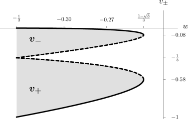
Figure 1: The admissible values of the rescaled isotropic pressure $w$ and $v_{-}$, $v_{+}=3w-2v_{-}$, which represent (the extremes of) the rescaled anisotropic pressures in the plane of symmetry and orthogonal to it, respectively. Both the strong and the dominant energy condition are satisfied. $(1-\sqrt{3})/3\approx-0.24$.

Results.

Since the dynamical system (11) extends regularly to $r=0$ it is suggestive to analyze the system induced on that surface. From (13) we obtain $H_{D}|_{r=0}=1$, $N_{1D}^{2}|_{r=0}=0$, so that (12) becomes $\Omega_{D}=1-\Sigma_{D}^{2}$. This in turn implies $q_{D}={\textstyle\frac{1}{2}}(1+3w)+{\textstyle\frac{3}{2}}(1-w)\Sigma_{D}^{2}$. Insertion into (11) yields

$$\Sigma_{D}^{\prime} =-3(1-\Sigma_{D}^{2})\Big{(}{\textstyle\frac{1}{2}}(1-w)\Sigma_{D}-\big{(}u(s)-w\big{)}\Big{)}\>,$$ (18a)

$$s^{\prime} =-12\Sigma_{D}\,s\left({\textstyle\frac{1}{2}}-s\right)\>.$$ (18b)

The state space for this two-dimensional dynamical system is $[-1,1]\times[0,1/2]$. The dynamical systems analysis is straightforward. We use that $u(s)$ is a function such that $u(0)=v_{-}$ and $u(1/2)=w+(w-v_{-})/2$; here, $w$ and $v_{-}$ are assumed to satisfy (16) and (17), respectively.

We focus our attention on the fixed point $\mathrm{R}$ of (18), which is given by

$$\mathrm{R}:r=0,\>s=0,\>\Sigma_{D}=-\beta\>.$$ (19)

It is straightforward to prove that $\mathrm{R}$ is a sink for the flow of the system (18), because

$$s^{-1}s^{\prime}\big{|}_{\mathrm{R}} =6\beta\,<\,0\>,$$ (20a)

$$(\Sigma_{D}+\beta)^{-1}(\Sigma_{D}+\beta)^{\prime}\big{|}_{\mathrm{R}} =-{\textstyle\frac{3}{2}}(1-\beta^{2})(1-w)\,<\,0\>,$$

hence the eigenvalues of the linearization of (18) at $$\mathrm{R}$$ are negative.

The crucial property of the fixed point $\mathrm{R}$ is revealed by considering the full system (11): $\mathrm{R}$ is a sink not only on the boundary $r=0$, but also for the full system (11). To see this we simply compute

$$r^{-1}r^{\prime}\big{|}_{\mathrm{R}}=2\Big{(}{\textstyle\frac{3}{2}}(1-w)\beta^{2}+{\textstyle\frac{1}{2}}(1+3w)+\beta\Big{)}<0$$ (20c)

and use (17) to establish that the r.h. side is negative.

Since the fixed point $\mathrm{R}$ is a sink for the flow of the system (11), i.e., for LRS Bianchi type IX models with anisotropic matter satisfying (16) and (17), there exists an open subset of LRS type IX initial data such that the corresponding solutions converge to $\mathrm{R}$. Because $H_{D}=1$ at $\mathrm{R}$ we infer from (13a) that $H$ is positive for these solutions for late times; by the remark following (9) we obtain that $H$ is positive, i.e., these models are expanding for all times.

In the following we analyze the asymptotic behavior of these forever expanding LRS type IX solutions in terms of the metric variables: For a solution of (11) that converges to the point $\mathrm{R}$ we find $r\rightarrow 0$, $s\rightarrow 0$, $\Sigma_{D}\rightarrow-\beta$, hence $H_{D}\rightarrow 1$, $N_{1D}\rightarrow 0$ by (13). Furthermore, $N_{2D}:=n_{2}/D\rightarrow\infty$; to see this we first note that $s\rightarrow 0$ implies $s\sim N_{1D}N_{2D}^{-1}$ by (7c). Then, from $N_{1D}\sim\sqrt{rs}$, see (13b), we conclude that $N_{2D}\sim\sqrt{r/s}$. Using that $s^{-1}s^{\prime}|_{\mathrm{R}}=6\beta$, cf. (20a), and $r^{-1}r^{\prime}|_{\mathrm{R}}=2(q+\beta)$, cf. (20c), where

$$q:=q_{D}\big{|}_{\mathrm{R}}={\textstyle\frac{3}{2}}(1-w)\beta^{2}+{\textstyle\frac{1}{2}}(1+3w)\>,$$

we finally get $N_{2D}^{-1}N_{2D}^{\prime}|_{\mathrm{R}}=q-2\beta>0$, and the claim follows. The fact that $N_{2D}=n_{2}/D\rightarrow\infty$ implies that $N_{2}:=n_{2}/H\rightarrow\infty$ as $\tau\rightarrow\infty$ since $H\simeq D$ in the limit (because $H_{D}=H/D=1$). This property is completely unproblematic here, but makes the treatment of the problem extremely difficult in the standard Hubble-normalized approach.

For large $\tau$, the shear variables are $\sigma_{1}=-2\sigma=-2D\Sigma_{D}\simeq 2D\beta$ and $\sigma_{2}=\sigma_{3}=\sigma=D\Sigma_{D}\simeq-D\beta$. To obtain the metric we integrate $\partial_{t}g_{kk}=2g_{kk}(H+\sigma_{k})$ (which is a consequence of $\partial_{t}g_{ij}=-2g_{il}k^{l}_{\>\,j}$). In the first step we note that $H=H_{D}D=D$ so that the equation reads $\partial_{t}g_{kk}=2g_{kk}(D+\sigma_{k})$, i.e.,

$$\partial_{\tau}g_{11}=2g_{11}(1+2\beta)\>,\quad\partial_{\tau}g_{22}=2g_{22}(1-\beta)\>.$$ (21)

Second, we integrate $D^{-1}D^{\prime}|_{\mathrm{R}}=-(1+q)$ and (8) to get $\tau=(1+q)^{-1}\log(t-t_{0})+\tau_{0}$ with constants $\tau_{0}$ and $t_{0}$. Therefore, (21) leads to an asymptotic behavior of the metric represented by

$$g_{11}\propto(t-t_{0})^{\frac{2(1+2\beta)}{1+q}}\>,\quad g_{22}\propto(t-t_{0})^{\frac{2(1-\beta)}{1+q}}$$ (22)

as $t\rightarrow\infty$. Note that $\beta$ is negative, but $1+2\beta$ is positive, which is a consequence of (17). An interesting observation is the occurence of partial (directional) accelerated expansion. A straightforward calculation reveals that $(1-\beta)/(1+q)>1$, hence lengths in the plane of local rotational symmetry expand at an accelerated rate. The maximal rate of acceleration is obtained by maximizing $(1-\beta)/(1+q)$ over the domain depicted in Fig. 1; the maximal value of $(1-\beta)/(1+q)\approx 1.112$ is attained for $w$ close to $-1/3$.

We conclude by restating the main result: The behavior (22) is typical, i.e., there exists an open set of LRS type IX initial data such that the associated solutions of the Einstein equations with anisotropic matter behave as (22) as $t\rightarrow\infty$ and thus expand forever. (These solutions do not behave extraordinarily in other respects; for instance, there exist forever expanding solutions that isotropize toward the singularity.) In this sense, eternal expansion is as likely as recollapse in the case of LRS Bianchi type IX with anisotropic matter that satisfies the conditions (16) and (17), and thus in particular the strong energy condition.

References

- (1) L. Amendola. Phantom Energy Mediates a Long-Range Repulsive Force. Phys. Rev. Lett., 93 : 181102, 2004.
- (2) J.D. Barrow. Cosmological limits on slightly skew stresses. Phys. Rev. D, 55 : 7451–7460, 1997.
- (3) J.D. Barrow, G.J. Galloway, and F.J. Tipler. The closed-universe recollapse conjecture. Mon. Not. R. Astron. Soc., 223 : 835–844, 1986.
- (4) S. Calogero and J.M. Heinzle. Bianchi cosmologies with anisotropic matter: Locally Rotationally Symmetric models. Preprint arXiv: 0911.0667.
- (5) S. Calogero and J.M. Heinzle. Dynamics of Bianchi type I solutions of the Einstein equations with anisotropic matter. Ann. Henri Poincaré, 10 : 225–274, 2009.
- (6) G.F.R. Ellis. General Relativity and Cosmology. R.K. Sachs, ed. New York Academic Press, 1971.
- (7) J.M. Heinzle, N. Röhr, and C. Uggla. Matter and dynamics in closed cosmologies. Phys. Rev. D, 71 : 083506, 2005.
- (8) X.f. Lin and R.M. Wald. Proof of the closed-universe-recollapse conjecture for diagonal Bianchi type IX cosmologies. Phys. Rev. D, 40 : 3280–3286, 1989.
- (9) R.J. Scherrer and A.A Sen. Phantom dark energy models with a nearly flat potential. Phys. Rev. D, 78 : 067303, 2008.
- (10) D.N. Vollick. How to produce exotic matter matter using classical fields. Phys. Rev. D, 56 : 4720–4723, 1997.
- (11) J. Wainwright and G.F.R. Ellis, editors. Dynamical systems in cosmology. Cambridge University Press, Cambridge, 1997.
- (12) R.M. Wald. General Relativity. The University of Chicago Press, 1984.