Collective effects of the Coulomb interaction in anharmonic quantum dots

Abstract

Deviations from the uniform oscillator spacing, related to the shape of the confining potential, have a strong influence on few-electron states in quantum dots when Coulomb effects are included. Distinct signatures are found for level spacings increasing (pot shape) and decreasing (cone shape) with energy. Cone deformations affect the levels near the ground state, such that observable effects are predicted. Pot deformations partially negate the effect of the Coulomb force, thus their spectra are similar to those of a perfect oscillator with a smaller Coulomb repulsion. The Coulomb force is treated by exact diagonalization, for which purpose efficient closed-form expressions for the matrix elements are derived. The Coulomb matrix element in relative coordinates is reduced to a single sum over four binomial coefficients, for which simple analytic approximations are found.

I Introduction

Quantum dots are both the smallest electronic devices, and the largest atoms. Technologically, they allow the storage and manipulation of single electrons. Physically, they are a practical laboratory to observe few-body Coulomb states at energy scales far below those of real light atoms. In small quantum dots, the Coulomb effects are typically about one-half of the oscillator spacing, so they have been treated perturbatively with success,Warburton et al. (1998) even though they would appear a priori to belong to a crossover regime.

More recent developments have stressed the role of electronic correlations in few-electron dots, among others with a view to manipulate quantum states for purposes of computation. Such efforts fall into two categories. One aims to construct “quantum dot molecules” in particular geometric patterns.Scheibner et al. (2007) The other has focussed on “electronic molecules,” referring to the limit of strongly interacting electrons within a single quantum dot, where a molecule-like partition of energy into rotational and vibrational degrees of freedom is observed.Kalliakos et al. (2009) These latter states might better be called “quantum dot nuclei,” since collectivization by the repulsive Coulomb force occurs in the absence of centers of opposite charge, which exist in molecules.

The present paper investigates the particular effect of well shape (in vertical, not horizontal profile), modelled as departure from the uniform single-particle energy spacing, on the collectivity of few-electron quantum states within a single dot. The modelling is implemented simply by inserting diagonal energy values, other than the “correct” oscillator ones. The two qualitatively different cases are level spacings increasing and decreasing with energy, referred to respectively as pot-shaped and cone-shaped dots.

The main result is that cone anharmonicities make quantum dots strongly prone to creation of collective states. The physical reason is first demonstrated on the classic case of two electrons (“quantum dot helium”), at modest values of the Coulomb force, consistent with the literature.Merkt et al. (1991) With four electrons, there appear both a change in ordering of the lowest excited states, and “intruder” states of exceptionally large spin and orbital momentum among the higher ones. Both of these should lead to observable effects, if such dots can be manufactured.

Two formal developments are also presented, which are not strictly necessary for the proof of principle given here, but may be useful in larger calculations. First, an advanced combinatorial techniqueWilf and Zeilberger (1992); Paule and Schorn (1995) is used to bring the center-of-mass (CM) Coulomb matrix elements to a more tractable form. It gives rise to two simple analytical approximations, one of them already known,Laughlin (1983) which give good estimates of the Coulomb matrix elements over a large range of quantum numbers. Second, a simple expression for the Coulomb matrix elements in laboratory coordinates is obtained, based on an old symmetry-based insight.Bakri (1967) The two together mean that binomial coefficients suffice in Coulomb calculations for the two-dimensional oscillator: no gamma or hypergeometric functions need apply.

II Center-of-mass matrix elements

The 2D oscillator Hamiltonian is

$$H_{\mathrm{osc}}=\left[-\frac{1}{2}\left(\frac{\partial^{2}}{\partial r^{2}}+\frac{1}{r}\frac{\partial}{\partial r}+\frac{1}{r^{2}}\frac{\partial^{2}}{\partial\phi^{2}}\right)+\frac{1}{2}r^{2}\right]\hbar\omega,$$ (1)

where the dimensionless coordinate $r$ has been scaled in units of the oscillator characteristic length $l_{0}=\sqrt{\hbar/(m\omega)}$. It has the eigenfunctions $\Psi_{nl}$,

$$\Psi_{nl}(\mathbf{r})=\Psi_{nl}(x,y)=\sqrt{\frac{n!}{\pi(n+l)!}}L^{l}_{n}(x^{2}+y^{2})(x+iy)^{l}e^{-(x^{2}+y^{2})/2},$$ (2)

where $L^{l}_{n}$ is the generalized Laguerre polynomial, and there are $2n+l+1$ degenerate eigenfunctions for each energy level:

$$H_{\mathrm{osc}}\Psi_{nl}=(2n+l+1)\hbar\omega\Psi_{nl}.$$ (3)

One can exploit a symmetry of the Laguerre polynomials,

$$(-1)^{k}\frac{k!}{x^{k}}L_{k}^{n-k}(x)=(-1)^{n}\frac{n!}{x^{n}}L_{n}^{k-n}(x),$$

to account for negative angular momenta in a natural way:

$$\Psi_{n,-l}=(-1)^{l}\Psi^{*}_{n-l,l}.$$ (4)

This allows one not to use absolute value signs on $l$, which is quite common in the literature, but would “break” all the main formulae in the present work. The notational price paid is that e.g. $\Psi_{11}$ and $\Psi_{1,-1}=-\Psi^{*}_{01}$ do not belong to the same energy level: the negative-momentum state corresponding to $\Psi_{11}$ is $\Psi_{2,-1}=-\Psi^{*}_{11}$.

To calculate two-body matrix elements, transform as usual to the CM frame,

$$\mathbf{R}=\frac{\mathbf{r}_{1}+\mathbf{r}_{2}}{\sqrt{2}},\quad\mathbf{r}=\frac{\mathbf{r}_{1}-\mathbf{r}_{2}}{\sqrt{2}}.$$ (5)

Denoting the CM basis $|NL;nl)=\Psi_{NL}(\mathbf{R})\Psi_{nl}(\mathbf{r})$, the Coulomb interaction turns out to be

$$\left(NL;nl\right|\frac{1}{|\mathbf{r}_{1}-\mathbf{r}_{2}|}\left|N^{\prime}L^{\prime};n^{\prime}l^{\prime}\right)=\delta_{NN^{\prime}}\delta_{LL^{\prime}}\delta_{ll^{\prime}}\sqrt{\frac{\pi}{2}}\frac{\sqrt{n!n^{\prime}!(n+l)!(n^{\prime}+l)!}}{(n+n^{\prime}+l)!}\left(\frac{1}{4}\right)^{n+n^{\prime}+l}\\ \times\sum_{j=0}^{\min(n,n^{\prime})}\binom{2n+2n^{\prime}-4j}{n+n^{\prime}-2j}\binom{n+n^{\prime}-2j}{n-j}\binom{4j+2l}{2j+l}\binom{2j+l}{j},$$ (6)

where Zeilberger’s algorithmWilf and Zeilberger (1992); Paule and Schorn (1995) was used to reduce the customary double sumPfannkuche et al. (1993) to a single one, as explained in Appendix A. Note that the sum has few terms in practice, since $n$ is at most one-half the principal quantum number $2n+l$. Dropping the CM quantum numbers $N,L$, which introduces a notation for the relative-coordinate wave functions, one observes

$$\left(n0\right|\frac{1}{|\mathbf{r}_{1}-\mathbf{r}_{2}|}\left|00\right)=\left(0n\right|\frac{1}{|\mathbf{r}_{1}-\mathbf{r}_{2}|}\left|0n\right),$$ (7)

which is quite noteworthy: the amplitude to scatter from the $2n$-th level to the ground state is the same as the energy shift felt by the state of maximal angular momentum in the $n$-th level. Thus the Coulomb force has the potential to mix states very strongly, and this is enhanced by the cone-shape anharmonicity, as explained below.

To get some feeling for the values involved, note that the inequality

$$\binom{2n}{n}<\frac{4^{n}}{\sqrt{n\pi}}$$ (8)

becomes an equality in the limit $n\to\infty$, i.e. is not an asymptotic expression. This provides the approximationLaughlin (1983)

$$\left(0n\right|\frac{1}{|\mathbf{r}_{1}-\mathbf{r}_{2}|}\left|0n\right)\sim\frac{1}{\sqrt{2n}}.$$ (9)

The energy shifts in states of smaller angular momentum are larger, but not by much, the largest, derived in Appendix B, being

$$\left(n0\right|\frac{1}{|\mathbf{r}_{1}-\mathbf{r}_{2}|}\left|n0\right)\sim\frac{1}{\sqrt{2n}}\left[\sqrt{2}+\frac{\ln n}{\pi}\right].$$ (10)

As shown in Fig. 1, the range of values of the diagonal Coulomb matrix elements is less than a factor of two, mostly given by the first (square root) factor in brackets. The analytic estimates are remarkably good, all the way down to $n=1$.

Figure 1: Coulomb matrix elements $\left(n0\right|\frac{1}{r\sqrt{2}}\left|n0\right)$ (upper points) and $\left(0n\right|\frac{1}{r\sqrt{2}}\left|0n\right)$ (lower points), along with their analytic estimates (full lines). The intermediate case $\left(n,n/10\right|\frac{1}{r\sqrt{2}}\left|n,n/10\right)$ is also shown for $n\geq 10$ (the step at $n=20$ comes from discretizing $n/10$). All matrix elements are in units of $\left<00\right|\frac{1}{r\sqrt{2}}\left|00\right>=\sqrt{\pi/2}$.

III Laboratory-frame matrix elements

Many-body wave functions in laboratory coordinates best exploit the symmetry between the particles. On the other hand, interaction terms in the Hamiltonian are more easily calculated in the CM frame, as above. Denoting the wave function in laboratory coordinates $\left|n_{1}l_{1};n_{2}l_{2}\right]=\Psi_{n_{1}l_{1}}(\mathbf{r}_{1})\Psi_{n_{2}l_{2}}(\mathbf{r}_{2})$, we need the transformation coefficients appearing in

$$\left|NL;nl\right)=\sum_{n^{\prime}=0}^{N+n}\quad\sum_{l^{\prime}=-n^{\prime}}^{N+L+n+l-n^{\prime}}C^{NL;nl}_{n^{\prime}l^{\prime}}\left|N+n-n^{\prime},L+l-l^{\prime};n^{\prime}l^{\prime}\right].$$ (11)

They can be found following the observationBakri (1967) that they must also appear in the transformation of the simplest monomial having the required symmetry, which is in this case

$$r^{2n+l}e^{il\phi}=(x-iy)^{n}(x+iy)^{n+l}.$$

One easily obtains, referring to Eq. (5),

$$(X-iY)^{N}(X+iY)^{N+L}(x-iy)^{n}(x+iy)^{n+l}=\\ \sum_{n^{\prime}l^{\prime}}d^{Nn}_{n^{\prime}}d^{N+L,n+l}_{n^{\prime}+l^{\prime}}(x_{1}-iy_{1})^{N+n-n^{\prime}}(x_{1}+iy_{1})^{N+L+n+l-n^{\prime}-l^{\prime}}(x_{2}-iy_{2})^{n^{\prime}}(x_{2}+iy_{2})^{n^{\prime}+l^{\prime}}$$ (12)

where

$$d^{Nn}_{n^{\prime}}=\frac{1}{\sqrt{2^{N+n}}}\sum_{m=\max(0,n^{\prime}-N)}^{\min(n,n^{\prime})}(-1)^{m}\binom{N}{n^{\prime}-m}\binom{n}{m}.$$ (13)

It follows that

$$C^{NL;nl}_{n^{\prime}l^{\prime}}=D^{Nn}_{n^{\prime}}D^{N+L,n+l}_{n^{\prime}+l^{\prime}},\quad D^{Nn}_{n^{\prime}}=\sqrt{\frac{\binom{N+n}{n}}{\binom{N+n}{n^{\prime}}}}d^{Nn}_{n^{\prime}},$$ (14)

where the square-root factors are needed to remove the standard normalizations of the wave functions, and Laguerre polynomials within them, so that the highest power of $r$ appears with coefficient unity, for the $d$’s to act upon as in Eq. (12). The inverse of the CM transformation, Eq. (5), looks the same, so the same expression (12) must hold upon exchanging $\mathbf{R}\leftrightarrow\mathbf{r}_{1}$ and $\mathbf{r}\leftrightarrow\mathbf{r}_{2}$, meaning that “)” and “]” can exchange places in Eq. (11). Thus, iterating Eq. (11) is the same as inverting it, i.e. the coefficients are idempotent:

$$\sum_{N=0}^{n_{1}+n_{2}}\quad\sum_{L=-N}^{n_{1}+l_{1}+n_{2}+l_{2}-N}C^{n_{1}l_{1};n_{2}l_{2}}_{NL}C^{n_{1}+n_{2}-N;l_{1}+l_{2}-L}_{N_{2}L_{2}}=\delta_{n_{2}N_{2}}\delta_{l_{2}L_{2}}.$$ (15)

Collecting the above results, one finds a computationally efficient expression for the matrix element in laboratory coordinates,

$$\left[n_{1}l_{1};n_{2}l_{2}\right|\frac{1}{|\mathbf{r}_{1}-\mathbf{r}_{2}|}\left|n_{3}l_{3};n_{4}l_{4}\right]=\\ \delta_{l_{1}+l_{2},l_{3}+l_{4}}\sum_{N=0}^{n_{1}+n_{2}}\quad\sum_{L=-N}^{n_{1}+l_{1}+n_{2}+l_{2}-N}C^{n_{1}l_{1};n_{2}l_{2}}_{NL}C^{n_{3}l_{3};n_{4}l_{4}}_{N+\Delta n,L}\left(NL\right|\frac{1}{|\mathbf{r}_{1}-\mathbf{r}_{2}|}\left|N+\Delta n,L\right),$$ (16)

where it is assumed that $\Delta n=n_{3}+n_{4}-n_{1}-n_{2}\geq 0$, without loss of generality.

IV The model

The model used for shape effects is a simple modification of the single-particle spectrum. The diagonal oscillator energies are modified to read

$$E(n,l,\delta)=(2n+l+1)^{1+\delta}\hbar\omega,$$ (17)

where $\delta=0$ is of course the original oscillator spectrum, and $\delta=1$ would correspond to the infinite-well spectrum, where the level energies increase quadratically with the principal quantum number. Thus positive values of $\delta$ are referred to as “pot-shaped” dots. Negative values of $d$ indicate level spacings decreasing with energy, and this is called “cone-shaped.” The extreme cone shape is the hydrogen spectrum, $\delta=-3$ (with a negative prefactor). The idea here is to vary $\delta$ in the more modest range $\delta=\pm 0.5$, with some reasonable effective Coulomb strength.

Concerning the latter, the operative parameter is

$$\alpha=\frac{1}{\epsilon}\frac{e^{2}/l_{0}}{\hbar\omega},$$ (18)

where $\epsilon$ is the relative dielectric constant of the parent material, and $l_{0}=\sqrt{\hbar/(m\omega)}$ is the oscillator length scale, so that $\alpha$ measures the Coulomb repulsion at well size in units of the oscillator spacing.

To summarize, the model considered in the present work is given by the Hamiltonian matrix

$$\left<A\right|H\left|B\right>=\left<A|B\right>\sum_{(n,l)\in A}\frac{E(n,l,\delta)}{\hbar\omega}+\alpha\left<A\right|V_{C}\left|B\right>,$$ (19)

where $A,B$ are Slater determinants in configuration space and $E(n,l,\delta)$ is the modified harmonic-oscillator spectrum, Eq. (17). Calculations are performed in the subspace of minimal spin projection (zero for even number of electrons), which is first broken down into blocks by diagonalizing the square of the total spin operator, thus identifying states by spin. This achieves the same economy as if one had generated a good spin basisTüreci and Alhassid (2006) at the beginning.

V Two electrons

Figure 2: Energy spectra of quantum dot helium, in dependence on the Coulomb strength $\alpha$. Left is the recalculated result of Ref. Merkt et al., 1991, with $\delta=0$ in Eq. (17), and only the first six excited states shown, the highest three degenerate. Right is the same with $\delta=-0.5$. All energies are relative to the ground state, which appears as a horizontal line. Successive levels in energy are drawn alternately by thin and thick lines. Five oscillator shells are included. Note that each “kink” on the higher curves in the right panel marks another level crossing, with even higher states, not shown.

Quantum dot helium, with only two electrons, is obviously not the best choice to demonstrate collective effects. However, it already points to the reason why cone deformations lead to enhanced collectivity. Figure 2 shows the evolution of the first six excited states as a function of Coulomb strength, in the usually investigated range $\alpha<10$.

There is an obvious overall scaling effect of the anharmonicity, so to compare with the harmonic case, one should set energy windows to contain the same number of states, rather than the same energy range. When this is done, as in Fig. 2, a clear qualitative difference emerges. The cone anharmonicity induces a much greater number of level crossings, and they shift to lower values of the Coulomb force.

The reason for the effect is that the higher oscillator shells open a larger phase space than the lower ones, and they fan out both up and down relative to the ground state. Simply enough, the states going down cross sooner with those coming up. Because there are many of them, the overall impact on the low-lying states is quite substantial, resulting in a multitude of level crossings where there have previously been only a few.

VI Four electrons

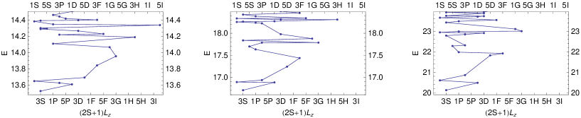
Figure 3: Energy spectra of four electrons for $\alpha=3$ and three values of $\delta$, left to right: $\delta=-0.5$, $\delta=0$, and $\delta=0.5$, respectively. The ground state is Hund’s rule triplet, denoted 3S. Note the inversion in order of the next three states in the left panel, and a 5I intruder, not appearing in the other two panels. The first $25$ states are shown in all three panels, connected by a full line in order of increasing energy. Four oscillator shells were used.

Predictably, the effect described in the previous section becomes more interesting with a larger number of electrons. Figure 3 shows a four-electron calculation, with $\delta=-0.5$, $\delta=0$, and $\delta=0.5$, left to right. The first thing that meets the eye is the loss of high orbital momentum states as $\delta$ increases, in particular the 3H state of the oscillator disappears upwards for the pot anharmonicity. Conversely, a 5I intruder moves down for the cone anharmonicity, to become the 16th excited state, while it was 36th in the harmonic oscillator.

Closer inspection reveals two remarkable peculiarities of the cone. First, while the 5I spin quintuplet has gone down in energy order, the 5S quintuplet, also present in the two other panels, has gone up, such that it is nearly degenerate with the 5I state of the cone. Calculation of electromagnetic transitions is beyond the scope of this work, but it is clear from general considerations that a 5S state lies in the decay path of a 5I state, because one can turn into the other by shedding orbital momentum only, without reconfiguring the spins. When they are nearly degenerate, decay of one into the other is likely to be significantly supressed, because of the scarcity of low-energy photons with the required high orbital momentum. This does not prove, without a calculation, that the 5I will have an anomalously long half-life, but does establish a plausible scenario for such an outcome.

The second cone peculiarity is the inversion of order of the first three excited states, which is 1D–1S–3P for the harmonic oscillator, and 1D–3P–1S for the cone. The interest here is that these states have recently been the subject of an extensive experimental analysis. Kalliakos et al. (2009) Thus cone-anharmonic dots have a qualitative fingerprint, in principle accesible to experiment, which may provide some motivation to try to manufacture them, and distinguish them experimentally from harmonic or pot-anharmonic ones.

The pot anharmonicity is much less interesting in comparison. Depletion of higher oscillator shell contributions suppresses the effects of the Coulomb force. The resulting spectra are similar to those obtained with a harmonic oscillator with a weaker Coulomb interaction.

VII Discussion and conclusion

The main result of this work is that cone anharmonicities in the single-particle level spacing of a quantum dot have a major impact on the collective effects, when the Coulomb force is taken into account. In the opposite limit, when the cone shape turns into a pot shape, the Coulomb force can be partially negated, and the spectrum recovers a form similar to the unperturbed oscillator with a smaller value of the interaction. In brief, cone deformations enhance Coulomb collective effects, pot deformations suppress them.

The physical mechanism leading to these effects is clear. Deviations from the single-particle spectrum, considered in this work, affect the higher oscillator shells more strongly. These are unoccupied in the non-interacting limit, for the fillings considered here. The stronger the interaction, the greater the admixture of the high shells to the ground state. Working against it is the energy price of involving them to optimize the occupied low level states. The benefit of even a slight reduction in their energy is high, because the higher shells have large degeneracies, so they make a lot of configuration space available for optimization. Conversely, when the component of high shells decreases, the space for interactions becomes more restricted, so the system behaves as if the Coulomb force were weaker than it is.

This interpretation is confirmed when one looks at the basis-vector composition of the low cone states, such as the 5I state in Fig. 3. Nothing dramatic happens with respect to the analogous oscillator state, only the higher (in single particle ordering) components are visibly more populated, and the lower ones, visibly less. However, simultaneous energy and wave-function rearrangements can have an order-of-magnitude impact on decay paths and lifetimes, providing a mechanism to establish time-limited “quantum protectorates”Laughlin and Pines (2000) with tunable properties.

The calculations are schematic in the sense that harmonic-oscillator wave functions do not diagonalize whichever potential would give the anharmonic diagonal energies, introduced by hand into the model. Nevertheless, it is not expected that the use of exact wave functions would affect the main outcome, because the mechanism described above is robust to model details. Furthermore, it is unlikely that the profile of a dot potential will ever be known with precision. The most that can be hoped is that some manufacturing prescription will turn out anharmonic dots with strongly collective charge states. If this happens, naturally one will assume that the potential well is cone-deformed. One might argue that the converse has already happened, and that the success of perturbation theory in describing real dots is partially due to the tendency of current manufacturing procedures towards pot-like anharmonicities, which suppress the collective effects of the Coulomb force.

While the effect itself is robust enough, its detailed outcomes appear to be quite uncontrolled. However, in practice it would not be necessary to achieve highly reproducible manufacturing to observe the effects discussed above. (Quantum dot molecular arrays are currently also produced with a considerable range of properties.Scheibner et al. (2008)) All that would be required to first order is that an acceptable percentage of manufactured dots have a tendency to “get stuck” in their de-excitation pathway. In any case, it is far-fetched at present to speculate on the possible ramifications of the simple proof of principle, given here. It is hoped, on the contrary, that its simplicity and universality will motivate someone to try to obtain strongly collective few-electron states by manufacturing anharmonic quantum dots with cone-like confining potentials.

Appendix A Coulomb interaction in relative coordinates

The usual expressionPfannkuche et al. (1993) for the Coulomb matrix element may be rewritten

$$\left(nl\right|\frac{1}{r\sqrt{2}}\left|n^{\prime}l^{\prime}\right)=\delta_{ll^{\prime}}\sqrt{\frac{\pi}{2}}\sqrt{n!n^{\prime}!(n+l)!(n+l^{\prime})!}\sum_{j=0}^{\min(n,n^{\prime})}\frac{1}{4^{2j+l}}\frac{(n+n^{\prime}-2j)!}{(n-j)!(n^{\prime}-j)!j!(l+j)!}S_{j},$$ (20)

where

$$S_{j}=\sum_{k=0}^{n+n^{\prime}-2j}\frac{(2l+2k+4j)!}{\left[(l+k+2j)!\right]^{2}(n+n^{\prime}-2j-k)!}\frac{(-1)^{k}}{4^{k}k!}.$$ (21)

Zeilberger’s algorithmWilf and Zeilberger (1992) givesPaule and Schorn (1995)

$$S_{j}=\frac{1}{16}\frac{(4j-2n-2n^{\prime}+1)(4j-2n-2n^{\prime}+3)}{(4j+2l+1)(4j+2l+3)(2j-n-n^{\prime})(2j-n-n^{\prime}+1)}S_{j+1},$$ (22)

which could in principle be checked directly. The solution is immediate,

$$S_{j}=\frac{(2n+2n^{\prime}-4j)!(4j+2l)!}{(n+n^{\prime}-2j)!^{2}(n+n^{\prime}+l)!(2j+l)!}\left(\frac{-1}{4}\right)^{n+n^{\prime}-2j}.$$ (23)

Inserting it above and rearranging terms into binomial coefficients gives Eq. (6). In checking the latter against the literature, one should take into account the caution below Eq. (4).

Appendix B Approximation for the zero-angular momentum matrix element

Using the approximation Eq. (8) for the case $l=0$ in Eq. (6), one easily finds

$$\left(n0\right|\frac{1}{r\sqrt{2}}\left|n0\right) \approx\frac{\sqrt{n}}{2\pi\sqrt{2}}\sum_{j=1}^{n-1}\frac{1}{j(n-j)}+\frac{\sqrt{2\pi}}{4^{2n}}\binom{4n}{2n}$$

$$\approx\frac{\sqrt{n}}{2\pi\sqrt{2}}\left(\sum_{j=1}^{n-1}\frac{1}{j(n-j)}+\frac{2\pi\sqrt{2}}{n}\right),$$ (24)

where the end terms in the sum are treated specially to preclude a nonsensical result. The sum is approximated by an integral,

$$\int_{1}^{n-1}\frac{1}{x(n-x)}dx=\frac{2\ln(n-1)}{n},$$

and finally $\ln(n-1)$ is replaced by $\ln n$ by inspection, because it gives a much better approximation.