On the equivalence between hierarchical segmentations and ultrametric watersheds

Abstract

We study hierarchical segmentation in the framework of edge-weighted graphs. We define ultrametric watersheds as topological watersheds null on the minima. We prove that there exists a bijection between the set of ultrametric watersheds and the set of hierarchical segmentations. We end this paper by showing how to use the proposed framework in practice on the example of constrained connectivity; in particular it allows to compute such a hierarchy following a classical watershed-based morphological scheme, which provides an efficient algorithm to compute the whole hierarchy.

Introduction

This paper is a contribution to a theory of hierarchical (image) segmentation in the framework of edge-weighted graphs. Image segmentation is a process of decomposing an image into regions which are homogeneous according to some criteria. Intuitively, a hierarchical segmentation represents an image at different resolution levels.

In this paper, we introduce a subclass of edge-weighted graphs that we call ultrametric watersheds. Theorem 5.5 states that there exists a one-to-one correspondence, also called a bijection, between the set of indexed hierarchical segmentations and the set of ultrametric watersheds. In other words, to any hierarchical segmentation (whatever the way the hierarchy is built), it is possible to associate a representation of that hierarchy by an ultrametric watershed. Conversely, from any ultrametric watershed, one can infer a indexed hierarchical segmentation.

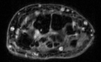
(a) Original image

(b) Dendrogram of the hierarchical segmentation

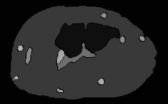
(c) One segmentation extracted from the hierarchy

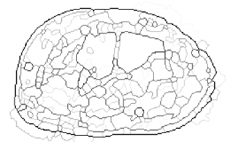
(d) An ultrametric watershed corresponding to the hierarchical segmentation

Figure 1: An example of a hierarchical segmentation produced by the method of L. Guigues GuiguesCM06 et al.. The classical order for reading the images is (a), (b), (c), (d). But Theorem 5.5 states that the reading order can also be (a), (d), (c), (b) (see text).

This theorem is illustrated on Fig. 1, that is produced using the method proposed in GuiguesCM06 : what is usually done is to compute from an original image (Fig. 1.a) a hierarchical segmentation that can be represented by a dendrogram (Fig. 1.b, see section 4). The borders of the segmentations extracted from the hierarchy (such as the one seen in Fig. 1.c) can be stacked to form a map (Fig. 1.d) that allows for the visual representation of the hierarchical segmentation. Theorem 5.5 gives a characterization of the class of maps (called ultrametric watersheds) that represent a hierarchical segmentation; more surprisingly, Theorem 5.5 also states that the dendrogram can be obtained after the ultrametric watershed has been computed.

Following BBO2004 , we can say that, independently of its theoretical interest, such a bijection theorem is useful in practice. Any hierarchical segmentation problem is a priori heterogeneous: assign to an edge-weighted graph an indexed hierarchy. Theorem 5.5 allows such classification problem to become homogeneous: assign to an edge-weighted graph a particular edge-weighted graph called ultrametric watershed. Thus, Theorem 5.5 gives a meaning to questions like: which hierarchy is the closest to a given edge-weighted graph with respect to a given measure or distance?

The paper is organised as follow. Related works are examined in section 1. We introduce segmentation on edges in section 2, and in section 3, we adapt the topological watershed framework from the framework of graphs with discrete weights on the nodes to the one of graphs with real-valued weights on the edges. We then define (section 4) hierarchies and ultrametric distances. In section 5, we introduce hierarchical segmentations and ultrametric watersheds, the main result being the existence of a bijection between these two sets (Th. 5.5). In the last part of the paper (section 6), we show how the proposed framework can be used in practice. After proposing (section 6.1) a convenient way to represent hierarchies as a discrete image, we demonstrate, using ultrametric watersheds, how to compute constrained connectivity Soille2007 as a classical watershed-based morphological scheme; in particular, it allows us to provide an efficient algorithm to compute the whole constrained-connectivity hierarchy.

Apart when otherwise mentionned, and to the best of the author’s knowledge, all the properties and theorems formally stated in this paper are new. This paper is an extended version of IGMI_Naj09 .

1 Related works

This section positions the proposed approach with respect to what has been done in various different fields. When reading the paper for the first time, it can be skipped. Readers with a background in classification will be interested in section 1.1, those with a background in hierarchical image clustering section 1.2, and those with a background in mathematical morphology by section 1.3.

1.1 Hierarchical clustering

From its beginning in image processing, hierarchical segmentation has been thought of as a particular instance of hierarchical classification Benzecri73 . One of the fundamental theorems for hierarchical clustering states that there exists a one-to-one correspondence between the set of indexed hierarchical classification and a particular subset of dissimilarity measures called ultrametric distances; This theorem is generally attributed to Johnson Johnson67 , Jardine et al. JardineSibson71 and Benzécri Benzecri73 . Since then, numerous generalisations of that bijection theorem have been proposed (see BBO2004 for a recent review).

Theorem 5.5 (see below) is an extension to hierarchical segmentation of this fundamental hierarchical clustering theorem. Note that the direction of this extension is different from what is done classically in hierarchical clustering. For example, E. Diday Diday2008 looks for proper dissimilarities that are compatible with the underlying lattice. An ultrametric watershed $F$ is not a proper dissimilarity, i.e. $F(x,y)=0$ does not imply that $x=y$ (see section 4). But $F$ is an ultrametric distance (and thus a proper dissimilarity) on the set of connected components of $\{(x,y)|F(x,y)=0\}$, those connected components being the regions of a segmentation.

Another point of view on our extension is the following: some authors assimilate classification and segmentation. We advocate that there exists a fundamental difference: in classification, we work on the complete graph, i.e. the underlying connectivity of the image (like the four-connectivity) is not used, and some points can be put in the same class because for example, their coordinates are correlated in some way with their color; thus a class is not always connected for the underlying graph. In the framework of segmentation, any region of any level of a hierarchy of segmentations is connected for the underlying graph. In other words, our approach yields a constrained classification, the constraint being the four-connectivity of the classes, or more generally any connection defining a graph (for the notion of connection and its links with segmentation, see Serra-2006 ; Ronse-2008 .)

1.2 Hierarchical segmentation

There exist many methods for building a hierarchical segmentation Pavlidis-1979 , which can be divided in three classes: bottom-up , top-down or split-and-merge. A recent review of some of those approaches can be found in Soille2007 . A useful representation of hierarchical segmentations was introduced in NS96 under the name of saliency map. This representation has been used (under several names) by several authors, for example for visualisation purposes GuiguesCM06 or for comparing hierarchies Arbelaez-Cohen-2006 .

In this paper, we show that any saliency map is an ultrametric watershed, and conversely.

1.3 Watersheds

For bottom-up approaches, a generic way to build a hierarchical segmentation is to start from an initial segmentation and progressively merge regions together PavlidisCh5-1977 . Often, this initial segmentation is obtained through a watershed meyer-beucher90 ; NS96 ; Meyer2005 . See meyer.najman:segmentation for a recent review of these notions in the context of mathematical morphology NajTal10 .

Among many others RM01 , topological watershed Ber05 is an original approach to watersheding that modifies a map (e.g., a grayscale image) while preserving the connectivity of each lower cross-section. It has been proved Ber05 ; NCB05 that this approach is the only one that preserves altitudes of the passes (named connection values in this paper) between regions of the segmentation. Pass altitudes are fundamental for hierarchical schemes NS96 . On the other hand, topological watersheds may be thick. A study of the properties of different kinds of graphs with respect to the thinness of watersheds can be found in CouBerCou2008 ; CouNajBer2008 . An useful framework is that of edge-weighted graphs, where watersheds are de facto thin (i.e. of thickness 1); furthermore, in that framework, a subclass of topological watersheds satisfies both the drop of water principle and a property of global optimality CouBerNaj2008a . In this subclass of topological watersheds, some of them can be seen as the limit, when the power of the weights tends to infinity for some specific energy function, of classical algorithms like graph cuts or random walkers CGNT09iccv ; CouGraNaj09c .

In this paper, we translate topological watersheds from the framework of vertice-weigthed-graphs to the one of edge-weighted graphs, and we identify ultrametric watersheds, a subclass of topological watersheds that is convenient for hierarchical segmentation.

2 Segmentation on edges

This paper is settled in the framework of edge-weighted graphs. Following the notations of Diestel97 , we present some basic definitions to handle such kind of graphs.

2.1 Basic notions

We define a graph as a pair $X=(V,E)$ where $V$ is a finite set and $E$ is composed of unordered pairs of $V$, i.e., $E$ is a subset of $\left\{\{x,y\}\subseteq V\;|\;x\neq y\right\}$. We denote by $|{V}|$ the cardinal of $V$, i.e, the number of elements of $V$. Each element of $V$ is called a vertex or a point (of $X$), and each element of $E$ is called an edge (of $X$). If $V\neq\emptyset$, we say that $X$ is non-empty.
As several graphs are considered in this paper, whenever this is necessary, we denote by $V(X)$ and by $E(X)$ the vertex and edge set of a graph $X$.
A graph $X$ is said complete if $E=V(X)\times V(X)$.
Let $X$ be a graph. If $u=\{x,y\}$ is an edge of $X$, we say that $x$ and $y$ are adjacent (for $X$). Let $\pi=\langle x_{0},\ldots,x_{\ell}\rangle$ be an ordered sequence of vertices of $X$, $\pi$ is a path from $x_{0}$ to $x_{\ell}$ in $X$ (or in $V$) if for any $i\in[1,\ell]$, $x_{i}$ is adjacent to $x_{i-1}$. In this case, we say that  $x_{0}$ and $x_{\ell}$ are linked for $X$. We say that  $X$ is connected if any two vertices of $X$ are linked for $X$.
Let $X$ and $Y$ be two graphs. If $V(Y)\subseteq V(X)$ and $E(Y)$ $\subseteq E(X)$, we say that  $Y$ is a subgraph of $X$ and we write $Y\subseteq X$. We say that $Y$ is a connected component of $X$, or simply a component of $X$, if $Y$ is a connected subgraph of $X$ which is maximal for this property, i.e., for any connected graph $Z$, $Y\subseteq Z\subseteq X$ implies $Z=Y$.
Let $X$ be a graph, and let $S\subseteq E(X)$. The graph induced by $S$ is the graph whose edge set is $S$ and whose vertex set is made of all points that belong to an edge in $S$, i.e., $(\{x\in V(X)\;|\;\exists u\in S,x\in u\},S)$.

Important remark. Throughout this paper $G=(V,E)$ denotes a connected graph, and the letter $V$ (resp. $E$) will always refer to the vertex set (resp. the edge set) of $G$. We will also assume that $E\neq\emptyset$.
Let $S\subset E$. In the following, when no confusion may occur, the graph induced by $S$ is also denoted by $S$.

Typically, in applications to image segmentation, $V$ is the set of picture elements (pixels) and $E$ is any of the usual adjacency relations, e.g., the 4- or 8-adjacency in 2D KR89 .

If $S\subset E$, we denote by  $\overline{S}$ the complementary set of $S$ in $E$, i.e., $\overline{S}=E\setminus S$.

2.2 Segmentation in edge-weigthed graphs

A deep insight on our work is that we are working with edges and not with points: the minimal unit which we want to modify is an edge. Indeed, what we need is a discrete space in which we can draw the border of a segmentation, so that we can represent that segmentation by its border; in other words, we want to be able to obtain the regions from their borders, and conversely. In that context, a desirable property is that the regions of the segmentation are the connected components of the complement of the border.

As illustrated in Fig. 2.b, this is not possible to achieve with the classical definition of a point-cut. Indeed, recall that a partition of $V$ is a collection ($V_{i}$) of non-empty subsets of $V$ such that any element of $V$ is exactly in one of these subsets, and that a point-cut is the set of edges crossing a partition. Even if we add the hypothesis that any $(V_{i},(V_{i}\times V_{i})\cap E)$ is a connected graph, a $V_{i}$ can be reduced to an isolated vertice, as the circled grey-point of Fig. 2.b. In that case, the complement of the point-cut, being a set of edges, does not contain that isolated vertice. The correct space to work with is the one of edges, and this motivates the following definitions.

Definition 2.1

A set $C\subset E$ is an (edge-)cut (of $G$) if each edge of $C$ is adjacent to two different nonempty connected components of $\overline{C}$. A graph $S$ is called an segmentation (of $G$) if $\overline{E(S)}$ is a cut. Any connected component of a segmentation $S$ is called a region (of $S$).

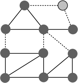
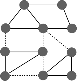
Figure 2: Illustration of segmentation and edge-cut. (a) A graph $X$. (b) A subgraph of $X$ which is not a segmentation of $X$: the circled grey-point is isolated, and if the point-cut $D$ is the set of dotted-lines edges, $\overline{D}$ contains only two connected components, instead of the expected three (see text). (c) An segmentation of $X$; the set $C$ of dotted-lines edges is the associated edge-cut of $X$.

As mentioned above, the previous definitions of cut and segmentation (illustrated on Fig. 2.c) are not the usual ones. One can remark the complement of the complement of a cut is the cut itself, and that any segmentation gives a partition, the converse being false. In particular, Prop. 2.2.i below states that there is no isolated point in an segmentation. If we need an isolated point $x$, it is always possible to replace $x$ with an edge $\{x^{\prime},y^{\prime}\}$. An application of the framework of hierarchical segmentation to constrained connectivity (where isolated points are present) is described in section 6.

It is interesting to state the definition of a segmentation from the point of view of vertices of the graph. A graph $X$ is said to be spanning (for $V$) if $V(X)=V$. We denote by $\phi$ the map that associates, to any $X\subset G$, the graph $\phi(X)=\{V(X),\{\{x,y\}\in E|x\in V(X),y\in V(X)\}\}$. We observe that $\phi(X)$ is maximal among all subgraphs of $G$ that are spanning for $V(X)$, it is thus a closing on the lattice of subgraphs of $G$ IGMI_CouNajSer09 . We call $\phi$ the edge-closing.

Property 2.2

A graph $S\subseteq G=(V,E)$ is a segmentation of $G$ if and only if

1. The graph induced by $E(S)$ is $S$;

2. $S$ is spanning for $V$;

3. for any connected component $X$ of $S$, $X=\phi(X)$.

Proof

Let $S$ be a segmentation of $G$. Then $\overline{S}$ is a cut, in other word, any edge $v=\{x,y\}\not\in E(S)$ is such that $x$ an $y$ are in two different connected components of $\overline{S}$. As $G$ is connected, that implies that $S$ is spanning for $V$. Moreover, $E(S)$ is the set of all edges of $S$, and as $S$ is spanning for $G$, the graph induced by $E(S)$ is $(V,E(S))=S$. Let $X$ be a connected component of $S$, suppose that there exists $v=\{x,y\}\in E$ such that $x$ and $y$ belong to $X$ and $v\not\in E(X)$. But then $v\not\in E(S)$ and thus $x$ and $y$ are in two different connected components of $S$, a contradiction.

Conversely, let $S$ be a graph satisfying (i), (ii) and (iii) and let $v=\{x,y\}\not\in E(S)$. As, by (ii), $S$ is spanning for $V$, assertion (iii) implies that $x$ and $y$ are in two different connected components of $\overline{E(S)}$. Assertion (i) implies that there is no isolated points in $S$, thus $\overline{S}$ is a cut and thus $S$ is a segmentation of $G$.∎

2.3 Binary watershed

Let $X$ be a subgraph of $G$. We note $X+u=(V(X)\cup u,E(X)\cup\{u\})$. In other words, $X+u$ is the graph whose vertice-set is composed by the points of $V(X)$ and the points of $u$, and whose edge-set is composed by the edges of $E(X)$ and $u$. An edge $u\in\overline{E(X)}$ is said to be W-simple (for $X$) (see Ber05 ) if $X$ has the same number of connected components as $X+u$.
A subgraph $X^{\prime}$ of $G$ is a thickening (of $X$) if:

• $X^{\prime}=X$, or if

• there exists a graph $X^{\prime\prime}$ which is a thickening of $X$ and there exists an edge $u$ W-simple for $X^{\prime\prime}$ and $X^{\prime}=X^{\prime\prime}+u$.

Thus, informally, a thickening $X^{\prime}$ of $X$ is obtained by iteratively adding to $X$ a sequence of edges $u_{1},\ldots,u_{n}$, i.e. $X^{\prime}=X+u_{1}+\ldots+u_{n}$, with the constraint that in the sequence $X_{0}=X$, $X_{n+1}=X_{n}+u_{n+1}$, the edge $u_{n+1}$ is W-simple for $X_{n}$.

A subgraph $X$ of $G$ such that there does not exist a W-simple edge for $X$ is called a binary watershed (of $G$).

The following property is a consequence of the definitions of segmentation and binary watershed.

Property 2.3

A graph $X\subseteq G=(V,E)$ is a segmentation of $G$ if and only if $X$ is a binary watershed of $G$ and if $X$ is induced by $E(X)$.

Proof

If $X$ is a segmentation, then $\overline{E(X)}$ is a cut; let $u\in\overline{E(X)}$, $u$ is adjacent to two different non-empty connected components of $E(X)$, in other word $u$ is not W-simple for $X$. Thus any segmentation is a binary watershed.

Conversely, let $X$ be a binary watershed, any $u\not\in E(X)$ is not W-simple for $X$ (and thus $u$ is adjacent to two different connected components of $X$). If furthermore $X$ is induced by $E(X)$ then $\overline{E(X)}$ is a cut.∎

Thus, starting from a set of edges $X$, a segmentation is obtained by iterative thickening steps until idempotence. The next section extends the binary watershed approach to edge-weighted graphs.

3 Topological watershed

3.1 Edge-weighted graphs

We denote by $\mathcal{F}$ the set of all maps from $E$ to $\mathbb{R}^{+}$ Given any $F\in\mathcal{F}$, the positive numbers $F(u)$ for $u\in E$ are called the weights and the pair $(G,F)$ an edge-weighted graph. Whenever no confusion can occur, we will denote the edge-weighted graph $(G,F)$ by $F$.

For applications to image segmentation, we take for weight $F(u)$, where $u=\{x,y\}$ is an edge between two pixels $x$ and $y$, a dissimilarity measure between $x$ and $y$ (e.g., $F(u)$ equals the absolute difference of intensity between $x$ and $y$; see CouBerNaj09 for a more complete discussion on different ways to set the map $F$ for image segmentation). Thus, we suppose that the salient contours are located on the highest edges of $(G,F)$.

Let $\lambda\in\mathbb{R}^{+}$ and $F\in\mathcal{F}$, we define $F[\lambda]=\{v\in E\;|\;F(v)\leq\lambda\}$. The graph (induced by) $F[\lambda]$ is called a (cross)-section of $F$. A connected component of a section $F[\lambda]$ is called a component of $F$ (at level $\lambda$).

We define ${\cal C}(F)$ as the set composed of all the pairs $[\lambda,C]$, where $\lambda\in\mathbb{R}^{+}$ and $C$ is a component of the graph $F[\lambda]$. We call altitude of $[\lambda,C]$ the number $\lambda$. We note that one can reconstruct $F$ from ${\cal C}(F)$; more precisely, we have:

$$F(v)=\min\{\lambda\;|\;[\lambda,C]\in{\cal C}(F),v\in E(C)\}$$ (1)

For any component $C$ of $F$, we set $h(C)=\min\{\lambda\;|\;[\lambda,C]$ $\in{\cal C}(F)\}$. We define ${\cal C}^{\star}(F)$ as the set composed by all $[h(C),C]$ where $C$ is a component of $F$. The set ${\cal C}^{\star}(F)$, called the component tree of $F$ Salembier-Oliveras-Garrido-1998 ; NajCou2006 , is a finite subset of ${\cal C}(F)$ that is widely used in practice for image filtering. Note that the previous equation (1) also holds for ${\cal C}^{\star}(F)$:

$$F(v)=\min\{\lambda\;|\;[\lambda,C]\in{\cal C}^{\star}(F),v\in E(C)\}$$ (2)

We will make use of the component tree in the proof of Pr. 5.4.

A (regional) minimum of $F$ is a component $X$ of the graph $F[\lambda]$ such that for all $\lambda_{1}<\lambda$, $F[\lambda_{1}]\cap E(X)=\emptyset$. We remark that a minimum of $F$ is a subgraph of $G$ and not a subset of vertices of $G$; we also remark that any minimum $X$ of $F$ is such that $|{V(X)}|>1$.

We denote by ${\cal M}({F})$ the graph whose vertex set and edge set are, respectively, the union of the vertex sets and edge sets of all minima of $F$. In Fig. 3, boxes are drawn around each of the minimum of ${\cal M}({F})$. Note that ${\cal M}({F})$ is induced by $E({\cal M}({F}))$. As a convenient notation, and when no confusion can occur, we will sometimes write $X\in{\cal M}({F})$ if $X$ is a connected component of ${\cal M}({F})$.

3.2 Topological watersheds on edge-weighted graphs

In that section, we extend the definition of topological watershed Ber05 to edge-weighted graphs, and we give an original characterization of topological watersheds in that framework (Th. 3.4).

Let $F\in\mathcal{F}$. An edge $u$ such that $F(u)=\lambda$ is said to be W-destructible (for $F$) with lowest value $\lambda_{0}$ if there exists $\lambda_{0}$ such that, for all $\lambda_{1}$, $\lambda_{0}<\lambda_{1}\leq\lambda$, $u$ is W-simple for $F[\lambda_{1}]$ and if $u$ is not W-simple for $F[\lambda_{0}]$.

A topological watershed (on $G$) is a map that contains no W-destructible edges.

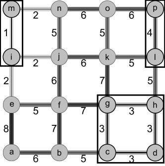
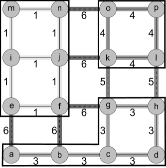
Figure 3: Illustration of topological watershed. (a) An edge-weighted graph $F$. (b) A topological watershed of $F$. The minima of (a) are $(\{m,i\}),(\{p,l\})$, $(\{g,h\},\{c,d\},\{g,c\},\{h,d\})$. A box is drawn around each one of the minimum in (a) and (b).

An illustration of a topological watershed can be found in Fig. 3.

A practical way to obtain a topological watershed from any given map is to apply a topological thinning, that, informally, consists in lowering W-destructible edges. More precisely, a map $F^{\prime}$ is a topological thinning (of $F$) if:

• $F^{\prime}=F$, or if

• there exists a map $F^{\prime\prime}$ which is a topological thinning of $F$ and there exists an edge $u$ W-destructible for $F^{\prime\prime}$ with lowest value $\lambda$ such that $\forall v\neq u,F^{\prime}(v)=F^{\prime\prime}(v)$ and $F^{\prime}(v)=\lambda_{0}$, with $\lambda\leq\lambda_{0}<F^{\prime\prime}(v)$.

A characterization of a W-destructible edge is provided through the connection value. The connection value between $x\in V$ and $y\in V$ is the number

$$F(x,y)=\min\{\lambda\;|\;[\lambda,C]\in{\cal C}(F),x\in V(C),y\in V(C)\}$$ (3)

In other words, $F(x,y)$ is the altitude of the lowest element $[\lambda,C]$ of ${\cal C}(F)$ such that $x$ and $y$ belong to $C$ (rule of the least common ancestor).

In Fig. 3.a and Fig. 3.b, it can be seen that the connection value between the points $m$ and $p$ is 6, that the one between $m$ and $d$ is 6, and that the one between $p$ and $d$ is $5$.

The connection value is a practical way to know if an edge is W-destructible. The following property is a translation of prop. 2 in CNB05 to the framework of edge-weighted graphs.

Property 3.1 (Prop. 2 in CNB05 )

Let $F\in\mathcal{F}$. An edge $v=\{x,y\}\in E$ is W-destructible for $F$ with lowest value $\lambda$ if and only if $\lambda=F(x,y)<F(v)$.

Two points $x$ and $y$ are separated (for $F$) if $F(x,y)>\max\{\lambda_{1},\lambda_{2}\}$, where $\lambda_{1}$ (resp. $\lambda_{2}$) is the altitude of the lowest element $[\lambda_{1},c_{1}]$ (resp. $[\lambda_{2},c_{2}]$) of ${\cal C}(F)$ such that $x\in c_{1}$ (resp. $y\in c_{2})$. The points $x$ and $y$ are $\lambda$-separated (for $F$) if they are separated and $\lambda=F(x,y)$.

The map $F^{\prime}$ is a separation of $F$ if, whenever two points are $\lambda$-separated for $F$, they are $\lambda$-separated for $F^{\prime}$.

If $X$ and $Y$ are two subgraphs of $G$, we set $F(X,Y)=\min\{F(x,y)\;|\;x\in X,y\in Y\}$.

Theorem 3.2 (Restriction to minima Ber05 )

Let $F^{\prime}\leq F$ be two elements of $\mathcal{F}$. The map $F^{\prime}$ is a separation of $F$ if and only if, for all distinct minima $X$ and $Y$ of ${\cal M}({F})$, we have $F^{\prime}(X,Y)=F(X,Y)$.

A graph $X$ is flat (for $F$) if for all $u,v\in E(X)$, $F(u)=F(v)$. If $X$ is flat, the altitude of $X$ is the number $F(X)$ such that $F(X)=F(v)$ for any $v\in E(X)$.

We say that $F^{\prime}$ is a strong separation of $F$ if $F^{\prime}$ is a separation of $F$ and if, for each $X^{\prime}\in{\cal M}({F^{\prime}})$, there exists $X\in{\cal M}({F})$ such that $X\subseteq X^{\prime}$ and $F(X)=F(X^{\prime})$.

Theorem 3.3 (strong separation Ber05 )

Let $F$ and $F^{\prime}$ in $\mathcal{F}$ with $F^{\prime}\leq F$. Then $F^{\prime}$ is a topological thinning of $F$ if and only if $F^{\prime}$ is a strong separation of $F$.

In other words, topological thinnings are the only way to obtain a watershed that preserves connection values.

In the framework of edge-weighted graphs, topological watersheds allows for a simple characterization.

Theorem 3.4

A map $F$ is a topological watershed if and only if:

1. ${\cal M}({F})$ is a segmentation of $G$;

2. for any edge $v=\{x,y\}$, if there exist $X$ and $Y$ in ${\cal M}({F})$, $X\neq Y$, such that $x\in V(X)$ and $y\in V(Y)$, then $F(v)=F(X,Y)$.

Proof

Let $F$ be a topological watershed. Thus there does not exist any edge W-destructible for $F$.

• Suppose that ${\cal M}({F})$ is not a segmentation of $G$. That means that there exists an edge $u=\{x,y\}\in\overline{E({\cal M}({F}))}$ such that $x$ and $y$ belongs to the same connected component $X$ of ${\cal M}({F})$. That implies that $F(u)>F(X)=F(x,y)$. By Pr. 3.1, that implies that the edge $u$ is W-destructible for $F$, a contradiction. Thus ${\cal M}({F})$ is a segmentation of $G$.

• As $F$ is a topological watershed, we have by Pr. 3.1 that for any $v=\{x,y\}\in E$, $F(x,y)=F(v)$. In particular, if there exist $X$ and $Y$ in ${\cal M}({F})$, $X\neq Y$, such that $x\in V(X)$ and $y\in V(Y)$, then $F(v)=F(X,Y)$.

Conversely, suppose that $F$ satisfies (i) and (ii). By Pr. 3.1, for any edge $v=\{x,y\}\in E({\cal M}({F}))$, $F(v)=F(x,y)=F(X)$, and thus ${\cal M}({F})$ does not contain any edge W-destructible for $F$. As, by (i), ${\cal M}({F})$ is a segmentation, any edge $v\not\in E({\cal M}({F}))$ satisfies (ii). By Pr. 3.1, such an edge $v$ is not W-destructible. Thus $F$ contains no W-destructible edge and is a topological watershed. ∎

Note that if $F$ is a topological watershed, then for any edge $v=\{x,y\}$ such that there exists $X\in{\cal M}({F})$ with $x\in V(X)$ and $y\in V(X)$, we have $F(v)=F(X)$.

4 Hierarchies and ultrametric distances

Let $\Omega$ be a finite set. A hierarchy $H$ on $\Omega$ is a set of parts of $\Omega$ such that

1. $\Omega\in H$

2. for every $\omega\in\Omega,\{\omega\}\in H$

3. for each pair $(h,h^{\prime})\in H^{2}$, $h\cap h^{\prime}\neq\emptyset\implies$ $h\subset h^{\prime}$ or $h^{\prime}\subset h$.

The (iii) can be expressed by saying that two elements of a hierarchy are either disjoint or nested.

An indexed hierarchy on $\Omega$ is a pair $(H,\mu)$, where $H$ denotes a given hierarchy on $\Omega$ and $\mu$ is a positive function, defined on $H$ and satisfying the following conditions:

1. $\mu(h)=0$ if and only if $h$ is reduced to a singleton of $\Omega$;

2. if $h\subset h^{\prime}$, then $\mu(h)<\mu(h^{\prime})$.

(a) Hierarchy

(b) Indexed hierarchy

Figure 4: Hierarchical trees. We have $\lambda_{1}<\lambda_{3}<\lambda_{4}$ and $\lambda_{2}<\lambda_{4}$.

Hierarchy are usually represented using a special type of tree called dendrograms (Fig. 4). The leafs of the tree are the data that are to be classified, while the branching point (the junctions) are the agglomeration of all the data that are below that point. In that sense, one can see that, for a given $h$, $\mu(h)$ corresponds to the “level” of aggregation, where the elements of $h$ have been aggregated for the first time.

Recall that a dissimilarity on $\Omega$ is a map $d$ from the Cartesian product $\Omega\times\Omega$ to the set $\mathbb{R}$ of real numbers such that: $d(\omega_{1},\omega_{2})=d(\omega_{2},\omega_{1})$, $d(\omega_{1},\omega_{1})=0$ and $d(\omega_{1},\omega_{2})\geq 0$ for all $\omega_{1},\omega_{2},\omega_{3}\in\Omega$. The dissimilarity $d$ is said to be proper whenever $d(\omega_{1},\omega_{2})=0$ implies $\omega_{1}=\omega_{2}$.

A distance $d$ (on $\Omega$) is a proper dissimilarity that obeys the triangular inequality $d(\omega_{1},\omega_{2})\leq d(\omega_{1},\omega_{3})+d(\omega_{3},\omega_{2})$ where $\omega_{1},\omega_{2}$ and $\omega_{3}$ are any three points of the space.

The ultrametric inequality Krasner1944 is stronger than the triangular inequality. An ultrametric distance (on $\Omega$) is a proper dissimilarity such that, for all $\omega_{1},\omega_{2},\omega_{3}\in\Omega$, $d(\omega_{1},\omega_{2})\leq\max(d(\omega_{1},\omega_{3}),d(\omega_{2},\omega_{3}))$

Note that any given partition ($\Omega_{i}$) of the set $\Omega$ induces a large number of trivial ultrametric distances: $d(\omega_{1},\omega_{1})=0,d(\omega_{1},\omega_{2})=1$ if $\omega_{1}\in\Omega_{i}$, $\omega_{2}\in\Omega_{j}$, $i\neq j$, and $d(\omega_{1},\omega_{2})=a$ if $i=j$, $0<a<1$. The general connection between indexed hierarchies and ultrametric distances goes back to Benzécri Benzecri73 and Johnson Johnson67 . They proved there is a bijection between indexed hierarchies and ultrametric distances, both defined on the same set. Indeed, associated with each indexed hierarchy $(H,\mu)$ on $\Omega$ is the following ultrametric distance:

$$d(\omega_{1},\omega_{2})=\min\{\mu(h)\;|\;h\in H,\omega_{1}\in h,\omega_{2}\in h\}.$$ (4)

In other words, the distance $d(\omega_{1},\omega_{2})$ between two elements $\omega_{1}$ and $\omega_{2}$ in $\Omega$ is given by the smallest element in $H$ which contains both $\omega_{1}$ and $\omega_{2}$. Conversely, each ultrametric distance $d$ is associated with one and only one indexed hierarchy.

Observe the similarity between Eq. 4 and Eq. 3. Indeed, connection value is an ultrametric distance on $V$ whenever $F>0$. More precisely, we can state the following property, whose proof is a simple consequence of Eq.4 and Eq. 3.

Property 4.1

Let $F\in\mathcal{F}$. Then $F(X,Y)$ is an ultrametric distance on ${\cal M}({F})$. If furthemore, $F>0$, then $F(x,y)$ is an ultrametric distance on $V$.

Let $\Psi$ be the application that associates to any $F\in{\cal F}$ the map $\Psi(F)$ such that for any edge $\{x,y\}\in E$, $\Psi(F)(\{x,y\})=F(x,y)$. It is straightforward to see that $\Psi(F)\leq F$, that $\Psi(\Psi(F))=\Psi(F)$ and that if $F^{\prime}\leq F$, $\Psi(F^{\prime})\leq\Psi(F)$. Thus $\Psi$ is an opening on the lattice $({\cal F},\leq)$ Leclerc81 . We observe that the subset of strictly positive maps that are defined on the complete graph $(V,V\times V)$ and that are open with respect to $\Psi$ is the set of ultrametric distances on $V$. The mapping $\Psi$ is known under several names, including “subdominant ultrametric” and “ultrametric opening”. It is well known that $\Psi$ is associated to the simplest method for hierarchical classification called single linkage clustering JardineSibson71 ; GR69 , closely related to Kruskal’s algorithm Kruskal56 for computing a minimum spanning tree.

Thanks to Th. 3.4, we observe that if $F$ is a topological watershed, then $\Psi(F)=F$. However, an ultrametric distance $d$ may have plateaus, and thus the weighted complete graph $(V,V\times V,d)$ is not always a topological watershed. Nevertheless, those results underline that topological watersheds are related to hierarchical classification, but not yet to hierarchical segmentation; the study of such relations is the subject of the rest of the paper.

5 Hierarchical segmentations, saliency and ultrametric watersheds

Informally, a hierarchical segmentation is a hierarchy of connected regions. However, in our framework, if a segmentation induces a partition, the converse is not true (see Pr. 2.2); thus, as the union of two disjoint connected subgraphs of $G$ is not a connected subgraph of $G$, the formal definition is slightly more involved.

A hierarchical segmentation (on $G$) is an indexed hierarchy $(H,\mu)$ on the set of regions of a segmentation $S$ of $G$, such that for any $h\in H$, $\phi(\cup_{X\in h}X)$ is connected ($\phi$ being the edge-closing defined in section 2).

For any $\lambda\geq 0$, we denote by $H[\lambda]$ the graph induced by $\{\phi(\cup_{X\in h}X)|h\in H,\mu(h)\leq\lambda\}$. The following property is an easy consequence of the definition of a hierarchical segmentation.

Property 5.1

Let $(H,\mu)$ be a hierarchical segmentation. Then for any $\lambda\geq 0$, the graph $H[\lambda]$ is a segmentation of $G$.

Proof

Let $(H,\mu)$ be a hierarchical segmentation, and let $\lambda\geq 0$. Suppose that $H[\lambda]$ is not a segmentation, i.e. that $\overline{H[\lambda]}$ is not a cut. Then there exists a connected component $X$ of $H[\lambda]$ and $v=\{x,y\}\in\overline{H[\lambda]}$ such that $x\in X$ and $y\in X$. That implies that $\phi(X)\neq X$, a contradiction with the definition of a hierarchical segmentation. ∎

Prop. 4.1 implies that the connection value defines a hierarchy on the set of minima of $F$. If $F$ is a topological watershed, then by Th. 3.4, ${\cal M}({F})$ is a segmentation of $G$, and thus from any topological watershed, one can infer a hierarchical segmentation. However, $F[\lambda]$ is not always a segmentation: if there exists a minimum $X$ of $F$ such that $F(X)=\lambda_{0}>0$, for any $\lambda_{1}<\lambda_{0}$, $F[\lambda_{1}]$ contains at least two connected components $X_{1}$ and $X_{2}$ such that $|{V(X_{1})}|=|{V(X_{2})}|=1$. Note that the value of $F$ on the minima of $F$ is not related to the position of the divide nor to the associated hierarchy of minima/segmentations. This leads us to introduce the following definition.

Definition 5.2

A map $F\in\mathcal{F}$ is an ultrametric watershed if $F$ is a topological watershed, and if furthemore, for any $X\in{\cal M}({F})$, $F(X)=0$.

Definition 5.2 directly yields to the nice following property, illustrated in Fig. 5, that states that any level of an ultrametric watershed is a segmentation and conversely.

Property 5.3

A map $F$ is an ultrametric watershed if and only if for all $\lambda\geq 0$, $F[\lambda]$ is a segmentation of $G$.

Proof

Suppose that $F$ is an ultrametric watershed, then it is a topological watershed, and by Th. 3.4.(i), ${\cal M}({F})$ is a segmentation of $G$. But as the value of $F$ on its minima is null, then any cross-section of $F$ is a segmentation of $G$.

Conversely, if for any $\lambda\geq 0$, $F[\lambda]$ is a segmentation of $G$, then $F$ contains no W-destructible edge for $F$. Indeed, suppose that there exists an edge $v$ W-destructible for $F$, let $\lambda=F(v)$, then $v$ is W-simple for $F[\lambda]$. In other words, adding $v$ to $F[\lambda]$ does not change the number of connected components of $F[\lambda]$. This is a contradiction with the definition of a segmentation. Hence $F$ is a topological watershed. Furthermore, as $F[\lambda]$ is a segmentation for any $\lambda\geq 0$, the value of $F$ on its minima is null, hence $F$ is an ultrametric watershed. ∎

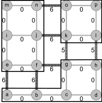
(a) Ultrametric watershed $F$

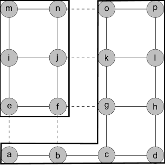
(b) cross-section of $F$ at level 5

Figure 5: An example of an ultrametric watershed $F$ and a cross-section of $F$. In (a), a box is drawn around each one of the minima of $F$, and in (b), a box is drawn around each one of the connected components of the cross-section of $F$. Remark that the minima of $F$, as well as any cross-section of $F$, form a segmentation of the graph.

By definition of a hierarchy, two elements of $H$ are either disjoint or nested. If furthermore $(H,\mu)$ is a hierarchical segmentation, the graphs $\overline{E(H[\lambda])}$ can be stacked to form a map. We call saliency map NS96 the result of such a stacking, i.e. a saliency map is a map $F$ such that there exists $(H,\mu)$ a hierarchical segmentation with $F(v)=\min\{\lambda|v\in E(H[\lambda])\}$.

Property 5.4

A map $F$ is a saliency map if and only if $F$ is an ultrametric watershed.

Proof

If $F$ is a saliency map, then there exists $(H,\mu)$ a hierarchical segmentation such that $F(v)=\min\{\lambda\;|\;v\in E(H(\lambda))\}$. But $F[\lambda]=\{v\;|\;F(v)\leq\lambda\}=\{v\;|\;\min\{\lambda\;|\;v\in E(H[\lambda])\}\leq\lambda\}=H[\lambda]$ and thus by Pr. 5.1, for any $\lambda\geq 0$, $F[\lambda]$ is a segmentation. By Pr. 5.3, $F$ is an ultrametric watershed.

Conversely, let $F$ be an ultrametric watershed, and let ${\cal C}^{\star}(F)$ be the component tree of $F$. We build the pair $(H,\mu)$ in the following way: $h\in H$ if and only if there exists $[\lambda,C]\in{\cal C}^{\star}(F)$ such that $h=\{X_{i}\;|\;X_{i}\in{\cal M}({F})\mbox{~{}and~{}}X_{i}\subset C\}$; in that case, we set $\mu(h)=\lambda$.

Then $(H,\mu)$ is a hierarchical segmentation. Indeed, let $h$ and $h^{\prime}$ two elements of $H$ such that there exists $[\lambda,X]$ and $[\lambda^{\prime},Y]$ in ${\cal C}^{\star}(F)$ with $h=\{X_{0},\ldots,X_{p}\;|\;X_{i}\in{\cal M}({F})\mbox{~{}and~{}}X_{i}\subset X\}$ and with $h^{\prime}=\{Y_{0},\ldots,Y_{n}\;|\;Y_{i}\in{\cal M}({F})\mbox{~{}and~{}}Y_{i}\subset Y\}$.

• by Th. 3.4, ${\cal M}({F})$ is a segmentation,

• we set $\lambda_{\max}=\max\{F(v)\;|\;v\in E\}$, it easy to see that $[\lambda_{\max},(V,E)]\in{\cal C}^{\star}(F)$, thus $\{\cup_{X\in{\cal M}({F})}\{X\}\}\in H$;

• any minimum $X$ of $F$ is such that $[0,X]$ belongs to ${\cal C}^{\star}(F)$, thus $\{X\}\in H$;

• furthermore, $h$ and $h^{\prime}$ are either disjoint or nested:

  • either disjoint: suppose that $X\cap Y=\emptyset$, in that case $h$ and $h^{\prime}$ are also disjoint;

  • or nested: suppose that $X\cap Y\neq\emptyset$, then as $X$ and $Y$ are two connected components of the cross-sections of $F$, either $X\subset Y$ or $Y\subset X$; suppose that $X\subset Y$; by reordering the $X_{i}$ and the $Y_{i}$, that means that $X_{i}=Y_{i}$ for $i=0,\ldots,p$, $p<n$. In other words, $h\subset h^{\prime}$.

• by construction, $\mu(h)=0$ if and only if there exists $X\in{\cal M}({F})$ such that $h=\{X\}$;

• If $h\subset h^{\prime}$, then $\mu(h)<\mu(h^{\prime})$, because in that case, $X\subset Y$ and thus $\lambda<\lambda^{\prime}$.

Thus $(H,\mu)$ is a indexed hierarchy on ${\cal M}({F})$.

Furthermore, $\phi(\cup_{X_{i}\in h}X_{i})$ is connected: more precisely, as ${\cal M}({F})$ is a segmentation, and as $X$ is a connected component of the cross-sections of $F$, we have $\phi(\cup_{X_{i}\in h}X_{i})=X$. Thus $(H,\mu)$ is a hierarchical segmentation. ∎

The following theorem, a corrolary of Prop. 5.4, states the equivalence between hierarchical segmentations and ultrametric watersheds. It is the main result of this paper.

Theorem 5.5

There exists a bijection between the set of hierarchical segmentations on $G$ and the set of ultrametric watersheds on $G$.

Proof

By Pr. 5.4, any ultrametric watershed is a saliency map, thus for any ultrametric watershed, there exists an associated hierarchical segmentation.

Conversely, for any hierarchical segmentation, there exists a unique saliency map, thus by Pr. 5.4, a unique ultrametric watershed. ∎

Th. 5.5 states that any hierarchical segmentation can be represented by an ultrametric watershed. Such a representation can easily be built by stacking the border of the regions of the hierarchy (see Pr. 5.1 and 5.4, but also NS96 ; GuiguesCM06 ; Arbelaez-Cohen-2006 ). More interestingly, Th. 5.5 also states that any ultrametric watershed yields a hierarchical segmentation. As the definition of topological watershed is constructive, this is an incentive to searching for algorithmic schemes that directly compute the whole hierarchy. An exemple of such an application of Th. 5.5 is developped in section 6.

As there exists a one-to-one correspondence between the set of indexed hierarchies and the set of ultrametric distances, it is interesting to search if there exists a similar property for the set of hierarchical segmentations. Let $d$ be the ultrametric distance associated to a hierarchical segmentation $(H,\mu)$. We call ultrametric contour map (associated to $(H,\mu)$) the map $d_{E}$ such that:

1. for any edge $v\in E(H[0])$, then $d_{E}(v)=0$;

2. for any edge $v=\{x,y\}\in\overline{E(H[0])}$, $d_{E}(v)=d(X,Y)$ where $X$ (resp. $Y$) is the connected component of $H[0]$ that contains $x$ (resp. $y$).

Property 5.6

A map $F$ is an ultrametric watershed if and only if $F$ is the ultrametric contour map associated to a hierarchical segmentation.

Proof

Let $F$ be an ultrametric watershed. By Pr. 4.1, $F(X,Y)$ is an ultrametric distance on ${\cal M}({F})$. By Pr. 5.3, $F$ is a saliency map, hence there exists a hierarchical segmentation $(H,\mu)$ such that $F(v)=\min\{\lambda\;|\;v\in E(H[\lambda])\}$. In particular,

1. for any edge $v\in E(H[0])$, then $F(v)=0$;

2. for any edge $v=\{x,y\}\in\overline{E(H[0])}$, $F(v)=F(X,Y)$ where $X$ (resp. $Y$) is the connected component of $H[0]$ that contains $x$ (resp. $y$).

Hence $F$ is an ultrametric contour map associated to a hierarchical segmentation.

Conversely, let $d_{E}$ be an ultrametric contour map associated to a hierarchical segmentation $(H,\mu)$. Then by Th. 3.4, $d_{E}$ is a topological watershed. Indeed, as $H$ is a hierarchical segmentation, $H[0]={\cal M}({d_{E}})$ is a segmentation of $G$, and furthermore for any edge $v=\{x,y\}$, if there exist $X$ and $Y$ in ${\cal M}({d_{E}})$, $X\neq Y$, such that $x\in V(X)$ and $y\in V(Y)$, then $d_{E}(v)=d(X,Y)=d_{E}(X,Y)$.

Moreover, for any $v\in{\cal M}({d_{E}})$, $d_{E}(v)=0$, hence $d_{E}$ is an ultrametric watershed. ∎

6 How to use the ultrametric watershed in practice: the example of constrained connectivity

Let us illustrate the usefulness of the proposed framework by providing an original way of revisiting constrained connectivity hierarchical segmentations Soille2007 , which leads to efficient algorithms. This section is meant as an illustration of our framework, and, although it is self-sufficient, technical details can be somewhat difficult to grasp for someone not familiar with the watershed-based segmentation framework of mathematical morphology meyer.najman:segmentation . We plan to provide more information in an extended version of that section.

In this section, we propose to compute an ultrametric watershed that corresponds to the constrained connectivity hierarchy of a given image. We show that, in the framework of edge-weighted segmentations, constrained connectivity can be thought as a classical morphological scheme, that consists of:

• computing a gradient;

• filtering this gradient by attribute filtering;

• computing a watershed of the filtered gradient.

We first discuss how to represent hierarchical segmentations, then give the formal definition of constrained connectivity, and then we move on to using ultrametric watersheds for computing such a hierarchy. In the last part of the section, we will show some other examples related to the classical watershed-based segmentation schemes.

6.1 Representations of hierarchical segmentations

As we mentionned in section 2.2, one of the motivations of this work is to be able to imbed the hierarchical segmentation in a discrete space in a way that can be represented. Until now, we have used the classical representation of a graph for all of our examples.

For the purpose of visualisation, it is enough to represent the image by a grid of double resolution. For example, with the usual four connectivity in 2D, each pixel will be the center of a 3x3 neighborhood, and if two pixels share an edge, the two corresponding neighborhoods will share 3 elements corresponding to that edge. The representation of an ultrametric watershed with double resolution can be seen in Fig. 6.a.

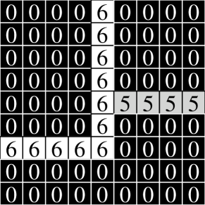
(a) Ultrametric watershed $F$ seen with double resolution

(b) Ultrametric watershed $F$ seen in the Khalimski grid

Figure 6: Two possible representations of the ultrametric watershed $F$ of Fig. 5.a.

Remark: A convenient interpretation of the doubling of the resolution can be given in the framework of cubical complexes, that have been popularized in computer vision by E. Khalimski KKM90 , but can be found earlier in the literature, originally in the work of P.S. Alexandroff AleHopf37 ; Ale37 .

Intuitively, a cubical complexe can be seen as a set of elements of various dimensions (cubes, squares, segments and points) with specific rules between those elements. The traditional vision of a numerical image as being composed of pixels (elementary squares) in 2D or voxels (elementary cubes) in 3D leads to a natural link between numerical images and complexes. The representation of an ultrametric watershed in the Khalimski grid can be seen in Fig. 6.b.

The framework of complexes is useful in the study of topological properties Ber07 . It is indeed possible to provide a formal treatment of watersheds in complexes, which we will not do in this paper. The interested reader can have a look at CBCN09iwcia .

6.2 Constrained connectivity

This section is a reminder of P. Soille’s approach Soille2007 , using the same notations.

Let $f$ be an application from $V$ to $\mathbb{R}$, i.e. an image with values on the points. For any set of points $U\subseteq V$, we set

$$R_{f}(U)=\sup\{f(x)-f(y)|x,y\in U\}.$$ (5)

The number $R_{f}(U)$ is called the range of $U$ (for $f$).

For any $x\in V$, and for any $\alpha\geq 0$, define NMI-1979 the $\alpha$-connected component $\alpha$-CC(x) as the set:

$$\alpha\mbox{-CC}(x)=\{x\}\cup\{y\in V |$$  there exists a path (6)

$$\pi=\{x_{0}=x,\ldots,x_{n}=y\},$$

$$n>0,\mbox{~{}such that~{}}$$

$$R_{f}(\{x_{i},x_{i+1}\})\leq\alpha,$$

$$\mbox{~{}for all~{}}0\leq i<n\}$$

An essential property of the $\alpha$-connected components of a point $x$ is that they form an ordered sequence (i.e a hierarchy) when increasing the value of $\alpha$:

$$\alpha\mbox{-CC}(x)\subseteq\beta\mbox{-CC}(x)$$ (7)

whenever $\beta\geq\alpha$. An example of such a hierarchy is given in Fig. 7.

Figure 7: Example from Soille2007 of a 7x7 image and its partitions into $\alpha$-connected components for $\alpha$ ranging from 0 to 5. (a) 0-CCs. (b) 1-CCs. (c) 2-CCs. (d) 3-CCs. (e) 4-CCs. (f) 5-CCs.

We now define the $(\alpha,\omega)$-connected component of an arbitrary point $x$ as the largest $\alpha$-connected component of $x$ whose range is lower that $\omega$; more precisely,

$$(\alpha,\omega)\mbox{-CC}(x)=\sup\{\beta\mbox{-CC}(x) | \beta\leq\alpha\mbox{~{}and~{}}$$ (8)

$$R_{f}(\beta\mbox{-CC}(x))\leq\omega\}$$

The $(\alpha,\omega)$-CCs also define a hierarchy, that is called a constrained connectivity hierarchy. We have:

$$(\alpha,\omega)\mbox{-CC}(x)\subseteq(\alpha^{\prime},\omega^{\prime})\mbox{-CC}(x)$$ (9)

whenever $\alpha^{\prime}\geq\alpha$ and $\forall\omega^{\prime}\geq\omega$. In practice Soille2007 , we are interested in this hierarchy for $\alpha=\omega$, i.e., for any $x\in V$ and any $\lambda\geq 0$, we are looking for ($\lambda,\lambda$)-CC(x).

Thus, informally, a hierarchy of $\alpha$-connected components is given by connectivity relations constraining gray-level variations along connected paths; a constrained connectivity hierarchy is given by connectivity relations constraining gray-level variations both along connected paths and within entire connected components.

An example of a constrained-connectivity hierarchy is given in Fig. 8.

Figure 8: Example from Soille2007 of a 7x7 image and its partitions into $(\alpha,\omega)$-connected components using identical values for the local and global range parameters ranging from 1 to 6. (a) (1, 1)-CCs. (b) (2, 2)-CCs. (c) (3, 3)-CCs. (d) (4, 4)-CCs. (e) (5, 5)-CCs. (f) (6, 6)-CCs.

6.3 Ultrametric watershed for constrained connectivity

In that section, we show how to build a weighted graph on which the ultrametric watershed corresponding to the hierarchy of constrained connectivity can be computed. Intuitively, this weighted graph can be seen as the gradient of the original image. We compute an ultrametric watershed for the hierarchy of $\alpha$-connected components. We filter that watershed to obtain the family of $(\alpha,\omega)$-connected components. We then show how to directly compute the ultrametric watershed corresponding to the hierarchy of $(\alpha,\omega)$-connected components.

Constrained connectivity is a hierarchy of flat zones of $f$, in the sense where the $0$-connected components of $f$ are the zones of $f$ where the intensity of $f$ does not change. In a continuous world, such zones would be the ones where the gradient is null, i.e. $\nabla f=0$. However, the space we are working with is discrete, and a flat zone of $f$ can consist in a single point. In general, it is not possible to compute a gradient on the points or on the edges such that this gradient is null on the flat zones. To compute a gradient on the edges such that the gradient is null on the flat zones, we need to “double” the graph, for example we can do that by doubling the number of points of $V$ and adding one edge between each new point and the old one (see Fig. 9(b)).

Figure 9: Doubling the graph. (a) Original graph with weights $f$ on the vertices. (b) Double graph, with weigths $f$ on the vertices and the gradient $F$ on the edges (see text).

More precisely, if we denote the points of $V$ by $V=\{x_{0},\ldots,x_{n}\}$, we set $V^{\prime}=\{x^{\prime}_{0},\ldots,x^{\prime}_{n}\}$ (with $V\cap V^{\prime}=\emptyset$), and $E^{\prime}=\{\{x_{i},x^{\prime}_{i}\}\;|\;0\leq i\leq n\}$. We then set $V_{1}=V\cup V^{\prime}$ and $E_{1}=E\cup E^{\prime}$. By construction, as $G=(V,E)$ is a connected graph, the graph $G_{1}=(V_{1},E_{1})$ is a connected graph.We also extend $f$ to $V^{\prime}$, by setting, for any $x^{\prime}\in V^{\prime}$, $f(x^{\prime})=f(x)$, where $\{x,x^{\prime}\}\in E^{\prime}$.

Let $(V_{1},E_{1},F)$ be the weighted graph obtained from $f$ by setting, for any $\{x,y\}\in E_{1}$, $F(\{x,y\})=|f(x)-f(y)|$. The map $F$ can be seen as the “natural gradient” of $f$ Mattiussi-2000 . It is easy to see that the flat zones of $f$, i.e. the $0$-connected components of $f$ are (in bijection with) the connected components of the set $\{v=\{x,y\}\in E_{1}\;|\;F(\{x,y\})=0\}$.

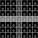
Figure 10: Doubling the graph as an image. (b) Doubling the graph of Fig. 9.a. (b) The gradient of (a) (see text).

Let us note that it is also possible, for the purpose of visualisation, to double the graph as an image, i.e., to multiply the size of the image by 2. On the graph of Fig. 9.a, that gives the image of Fig. 10.a. Then the gradient can be seen as an image (Fig. 10.b) as described in section 6.1. This representation will be adopted in all the subsequent figures of the paper.

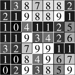
(a) Original image

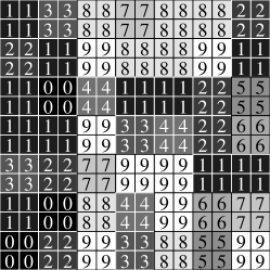
(b) Doubled image

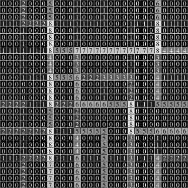
(c) Gradient

(d) Ultrametric watershed for the $\alpha$-connectivity

(e) Ultrametric watershed for the constrained connectivity

Figure 11: Example of a constrained connectivity hierarchy. (a) Original image (the one of Fig. 7) from Soille2007 . (b) Doubling of (a). (c) Gradient of (b). (d) Topological watershed of the gradient, that is the ultrametric watershed $W^{1}$ for the $\alpha$-connectivity that. (e) Ultrametric watershed $W^{2}$ for the constrained connectivity. (see text)

Let $W^{1}$ be a topological watershed of $F$. From Th. 3.4 and Eq. 3, if $W^{1}(\{x,y\})=\lambda$, there exists a path $\pi=\{x_{0}=x,\ldots,x_{n}=y\}$ linking $x$ to $y$ such that the altitude of any edge along $\pi$ is below $\lambda$, i.e. we have, for any $0\leq i<n$, $F(\{x_{i},x_{i+1}\})=|f(x_{i})-f(x_{i+1})|\leq\lambda$. The following property, the proof of which is left to the reader, states that the hierarchy of $\alpha$-connected components is given by $W^{1}$.

Property 6.1

We have

• $W^{1}$ is an ultrametric watershed;

• $W^{1}$ is uniquely defined (if $W^{\prime}$ is a topological watershed of $F$, then $W^{\prime}=W^{1}$);

• let $\lambda\geq 0$ and let $X$ be a connected component of the cross-section $W^{1}[\lambda]$; then for any $x\in V(X)\setminus V^{\prime}$, $\lambda\mbox{-CC}(x)=V(X)\setminus V^{\prime}$.

Pr. 6.1 is illustrated on Fig. 11.d. Let us stress that Fig. 11.d sums up in one image all the images of Fig. 7.

(a) Original image

(b) $W^{1}$(logarithmic grey-scale)

(c) $W^{2}$

(d) Area-filtering ultrametric watershed

Figure 12: Soille’s ($\alpha,\omega$)-constrained connectivity hierarchy. (a) Original image. (b) Ultrametric watershed $W^{1}$ for the $\alpha$-connectivity. (c) Ultrametric watershed $W^{2}$ for the constrained connectivity. (d) Ultrametric watersheds corresponding to one of the possible hierarchies of area-filterings on $W^{2}$.

One can notice that $R_{f}$ is increasing on $2^{V}$, i.e. $R_{f}(X)\subset R_{f}(Y)$ whenever $X\subseteq Y$. Thus $R_{f}$ is increasing on ${\mathcal{C}}(W^{1})$, and by removing the connected components of ${\cal C}(W^{1})$ that are below a threshold $\omega$ for $R_{f}$, we have an attribute filtering which is idempotent (the values on the points do not change), thus it is a closing. More precisely, we denote by $(R_{\lambda})_{\lambda\geq 0)}$ the family of maps obtained by applying this closing on $W^{1}$ for varying $\lambda$, i.e., for any $\lambda\geq 0$ and any $\{x,y\}\in E_{1}$, we set

$$R_{\lambda}(\{x,y\})=\min\{\lambda^{\prime} \;|\; [\lambda^{\prime},C]\in{\cal C}(W^{1}),$$ (10)

$$x\in V(C),y\in V(C),$$

$$R_{f}(V(C))\geq\lambda\}$$

In other words, the altitude for $R_{\lambda}$ of the edge $\{x,y\}$ is the altitude of the lowest component of ${\cal C}(W^{1})$ that contains both $x$ and $y$ and such that the range of that component is greater than $\lambda$.

The family $(R_{\lambda})_{\lambda\geq 0}$ allows us to retrieve the $(\alpha,\omega)$-CCs of $f$: surprisingly, it can be shown that any $R_{\lambda}$ is a topological watershed, and thus ${\cal M}({R_{\lambda}})$ is a segmentation from which it is easy to extract the $(\lambda,\lambda)$-connected component of a point, as the minimum of ${\cal M}({R_{\lambda}})$ that contains that point (See Pr. 6.2 below for a more formal setting).

Moreover, one can directly compute the ultrametric watershed associated to the hierarchy of $(\alpha,\omega)$-constrained connectivity. We set:

$$W^{2}(\{x,y\})=\min\{R_{f}(V(C)) \;|\; [\lambda,C]\in{\cal C}(W^{1}),$$ (11)

$$x\in V(C),$$

$$y\in V(C)\}$$

In other words, the altitude for $W^{2}$ of the edge $\{x,y\}$ is the range of the lowest component of ${\cal C}(W^{1})$ that contains both $x$ and $y$. One can remark that Eq. 11 corresponds to Eq. 8 for the framework of segmentation.

The following property, the proof of which is left to the reader, states that the hierarchy of $(\alpha,\omega)$-connected components is given by $W^{2}$.

Property 6.2

We have

• $\forall\lambda\geq 0$, $R_{\lambda}$ is a topological watershed;

• $\forall\lambda\geq 0$, $W^{2}[\lambda]={\cal M}({R_{\lambda}})$ ;

• $W^{2}$ is an ultrametric watershed;

• $W^{2}$ is uniquely defined;

• let $\lambda\geq 0$ and let $X$ be a connected component of the cross-section $W^{2}[\lambda]$; then for any $x\in V(X)\setminus V^{\prime}$, $(\lambda,\lambda)\mbox{-CC}(x)=V(X)\setminus V^{\prime}$.

Prop. 6.2, illustrated on Fig. 11.e, thus gives an efficient algorithm to compute the hierarchy of $(\alpha,\omega)$-constrained connectivity. Indeed, Eq. 11 can be computed in constant time BenderFarach-Colton-2000 on ${\cal C}(W^{1})$, which itself can be computed in quasi-linear time NajCou2006 . Such an algorithm is much faster than the one proposed in Soille2007 , that computes only one level of the hierarchy.

Let us stress that for an algorithmic/implementation point of view, it is not necessary in practice to double the image. Furthermore, for an efficient computation of the hierarchy, a minimum spanning tree or a component tree of the gradient can also be used instead of an ultrametric watershed, without changing the overall theoretical complexity of the algorithm. But for visualisation purpose, the ultrametric watershed is necessary. Moreover, those tools can be combined; indeed, one can compute a topological watershed on the graph of a minimum spanning tree. In a forthcomming paper, we will propose various data structures, including but not limited to component tree and minimum spanning tree, that allows an efficient computation of hierarchical segmentations. We will also study how to extend Prop. 6.2 in order to compute any granulometry of operators (strong hierarchies in the sense of Serra-2006 ).

A example of the application of the properties of this section to a real image is given in Fig. 12. Visualising $W^{2}$ allows to assess some of the qualities of the hierarchy of constrained connectivity. One can notice in Fig. 12.c a large number of transition regions (small undersirable regions that persist in the hierarchy), and this problem is known Soille-Grazzini-2009 . As $W^{2}$ is an image, a number of classical morphological schemes (e.g., area filtering that produces a hierarchy of regions classified according to their size or area; see meyer.najman:segmentation for more details) can be used to remove those transition zones (see Fig. 12.d for an example). Studying the usefulness of such schemes is the subject of future research.

6.4 Links with other hierarchical schemes

As we have shown, and as stated by Th. 5.5, any hierarchical scheme can be represented by and computed through an ultrametric watershed. This is in particular true for the classical watershed-based segmentation algorithms.

Fig. 13 is an illustration of the application of the framework developped in this paper to a classical hierarchical segmentation scheme based on attribute opening NS96 ; Salembier-Oliveras-Garrido-1998 ; meyer.najman:segmentation . The attribute opening tends to produce large plateaus where a watershed can be located anywhere; in particular, the contours at a given level of the hierarchy can be choosen differently depending on the filtering level, and one has to take care of indeed producing a hierarchy. In contrast, the ultrametric watershed will always choose a contour that is present at a lower level of the hierarchy.

Fig. 14 shows some of the differences between applying an ultrametric-watershed scheme and applying a classical watershed-based segmentation scheme, e.g. attribute opening followed by a watershed meyer-beucher90 . As watershed algorithms generally place watershed lines in the middle of plateaus, the contours produced by the classical watershed-based segmentation scheme do not lead to a hierarchy, and the two schemes give quite different results.

(a) Original image

(b) Ultrametric watershed

(c) Cross section of (b)

Figure 13: Example of ultrametric watershed. On (a), a box is drawn around the zoomed part used in Fig. 14

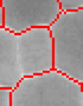
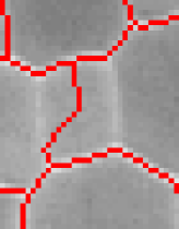
Figure 14: Zoom on a comparison between two watersheds of a filtered version of the image 13.a. Morphological filtering tends to create large plateaus, and both watersheds (a) and (b) are possible, but only (a) is a subset of a watershed of 13.a. No hierarchical scheme will ever give a result as (b).

7 Conclusion

In this paper, we have shown (Th. 5.5) that any hierarchical segmentation can be represented by an ultrametric watershed, and conversely that any ultrametric watershed leads to a hierarchical segmentation. Th. 5.5 thus offers an alternative way of thinking hierarchical segmentation that complete existing ones (ultrametric distances, minimum spanning tree, $\ldots$) We have seen how to apply Th. 5.5 to directly compute the constrained connectivity hierachy as an ultrametric watershed, leading to a fast algorithm. An important research direction is to provide a generalization of this scheme for computing any hierachical segmentation.

As a step in this direction, future work will propose novel algorithms (based on the topological watershed algorithm CNB05 ) to compute ultrametric watersheds, with proof of correctness. It is important to note that most of the algorithms proposed in the literature to compute saliency maps are not correct, often because they rely on wrong connection values or because they rely on thick watersheds where merging regions is difficult CouBerCou2008 .

On a more theoretical level, this work can be pursued in several directions.

• We will study lattices of watersheds IGMI_CouNajSer08 and will bring to that framework recent approaches like scale-sets GuiguesCM06 and other metric approaches to segmentation Arbelaez-Cohen-2006 . For example, scale-sets theory considers a rather general formulation of the partitioning problem which involves minimizing a two-term-based energy, of the form $\lambda C+D$, where $D$ is a goodness-of-fit term and $C$ is a regularization term, and proposes an algorithm to compute the hierarchical segmentation we obtain by varying the $\lambda$ parameter. As in the case of constrained connectivity (see section 6 above), we can hope that the topological watershed algorithm CNB05 can be used on a specific energy function to directly obtain the hierarchy.

• Subdominant theory (mentionned at the end of section 4) links hierarchical classification and optimisation. In particular, the subdominant ultrametric $d^{\prime}$ of a dissimilarity $d$ is the solution to the following optimisation problem for $p<\infty$:

  $$\min\{||d-d^{\prime}||_{p}^{p} \;|\; d^{\prime}\mbox{~{}is an ultrametric distance }$$ (12)

  $$\mbox{~{}~{} and~{}}d^{\prime}\leq d\}$$

  It is certainly of interest to search if topological watersheds can be solutions of similar optimisation problems.

• Several generalisations of hierarchical clustering have been proposed in the literature BBO2004 . An interesting direction of research is to see how to extend in the same way the topological watershed approach, for example for allowing regions to overlap.

• Last, but not least, the links of hierarchical segmentation with connective segmentation Serra-2006 have to be studied.

Laurent Najman received the Habilitation à Diriger les Recherches in 2006 from University the University of Marne-la-Vallée, the Ph.D. degree in applied mathematics from Université Paris-Dauphine in 1994 with the highest honor (Félicitations du Jury) and the engineering degree from the Ecole Nationale Supérieure des Mines de Paris in 1991. He worked in the central research laboratories of Thomson-CSF for three years after his engineering degree, working on infrared image segmentation problems using mathematical morphology. He then joined a start-up company named Animation Science in 1995, as director of research and development. The particle systems technology for computer graphics and scientific visualization developed by the company under his technical leadership received several awards, including the “European Information Technology Prize 1997” awarded by the European Commission (Esprit programme) and by the European Council for Applied Science and Engineering as well as the “Hottest Products of the Year 1996” awarded by the Computer Graphics World journal. In 1998, he joined OCÉ Print Logic Technologies, as senior scientist. There he worked on various image analysis problems related to scanning and printing. In 2002, he joined the Informatics Department of ESIEE, Paris, where he is professor and a member of the Gaspard-Monge computer science research laboratory (LIGM), Université Paris-Est. His current research interest is discrete mathematical morphology.