Lie groups in nonequilibrium thermodynamics: Geometric structure behind viscoplasticity

Abstract

Poisson brackets provide the mathematical structure required to identify the reversible contribution to dynamic phenomena in nonequilibrium thermodynamics. This mathematical structure is deeply linked to Lie groups and their Lie algebras. From the characterization of all the Lie groups associated with a given Lie algebra as quotients of a universal covering group, we obtain a natural classification of rheological models based on the concept of discrete reference states and, in particular, we find a clear-cut and deep distinction between viscoplasticity and viscoelasticity. The abstract ideas are illustrated by a naive toy model of crystal viscoplasticity, but similar kinetic models are also used for modeling the viscoplastic behavior of glasses. We discuss some implications for coarse graining and statistical mechanics.

1 Which mathematics behind which physics?

The purpose of this work is to explore an elaborate mathematical framework and its basic concepts in order to illuminate some physics and to develop a natural and general scenario for a range of phenomena. The underlying mathematics is the abstract theory of Lie groups and, in particular, the correspondence between Lie groups and Lie algebras. Our concrete interest is in groups of space transformations. The physics associated with space transformations is the theory of deformation of materials, ranging from fluids to solids and encompassing all kinds of intermediate behavior. We are thus dealing with elasticity theory and rheology, viscoelasticity, viscoplasticity, and all that. We here make an attempt at classifying models and phenomena in rheology from a mathematical perspective. The key idea is that we identify discrete groups of equivalent reference states that evolve slowly in time, much slower than the structural variables describing deviations from the reference states. We lay the foundations for the kinetic theory of systems with reference states so that it becomes possible to bridge the gap between atomistic and phenomenological models of viscoplasticity.

Lie algebras are known to play an important role in the theory of complex fluids [19]. Lie algebras allow us to introduce Poisson brackets and Poisson brackets allow us to introduce reversible dynamics (see Sec. 3 for details). With the help of a Poisson bracket, an energy function generates Hamiltonian dynamics, which is the prototype of mechanistically controlled or reversible dynamics, to be separated from the irreversible “rest” in any thermodynamics. Nonequilibrium thermodynamics can take place only in structured spaces, more precisely, thermodynamic systems must possess a Poissonian structure. This geometric structure is rooted in Lie algebras. More carefully, one should consider not only Lie algebras but also Lie groups, because one is usually working in infinite-dimensional spaces: Not every infinite-dimensional representation of a Lie algebra is guaranteed to exponentiate to a representation of some group (see §6.5 of Rossmann [25]). The relevant Poisson brackets are actually obtained by a procedure known as Lie-Poisson reduction from the canonical Poisson bracket on the cotangent bundle of a Lie group [15, 19], so that a group, or a representation of a group, is the true starting point for providing structure in nonequilibrium thermodynamics even though the final Poisson bracket is given in terms of the Lie algebra.

Once one is aware of the fact that thermodynamics requires structured spaces associated with Lie groups and their Lie algebras, it is natural to look at all possible Lie groups associated with a given Lie algebra. These groups can actually be characterized very nicely [8, 25]. There is a unique simply connected universal covering group $\mathcal{G}$, and all groups with the same Lie algebra are isomorphic to a quotient group of the form ${\mathcal{G}}/{\mathcal{Z}}$, where $\mathcal{Z}$ is a finite or infinite discrete normal subgroup of $\mathcal{G}$ (a subgroup ${\mathcal{Z}}\subset{\mathcal{G}}$ is normal if $gzg^{-1}\in{\mathcal{Z}}$ for all $z\in{\mathcal{Z}}$ and $g\in{\mathcal{G}}$). Actually, $\mathcal{Z}$ must be contained in the center of the group $\mathcal{G}$, that is, all elements of $\mathcal{Z}$ commute with all elements of $\mathcal{G}$ (or, $gzg^{-1}=z$; see §2.6 of Rossmann [25]). What is the physical significance of the groups $\mathcal{Z}$ and ${\mathcal{G}}/{\mathcal{Z}}$ in our application of group theory? Why can we interpret the elements of the discrete group $\mathcal{Z}$ as reference states?

For illustration, let us consider the subgroup of unidirectional shear deformations of a simple cubic lattice in one of its principal directions, ${\mathcal{G}}={\rm I\!R}$, with addition as the binary group operation. For small shear deformations, we expect elastic behavior. For a unit shear deformation between neighboring lattice planes, we reach a state that is fully equivalent to the undeformed state and, therefore, such a unit shear deformation is plastic. The discrete normal subgroup of integers, ${\mathcal{Z}}={\sf ZZ}$, represents a set of equivalent reference states, and ${\rm I\!R}/{\sf ZZ}=I_{0}=[-1/2,1/2[$ describes shear deformations with respect to a reference state. The topology of the Lie group ${\rm I\!R}/{\sf ZZ}$ (with the identification of $-1/2$ and $1/2$) is that of a circle, which is not simply connected. The occurrence of discrete subgroups is a general mathematical feature and it is natural to associate them with the equivalent reference configurations of a lattice. Only the simply connected universal covering group is free of reference states and hence provides the natural setting for viscoelastic liquids and other complex fluids. All smaller groups are associated with reference states and viscoplasticity.

The detailed elaboration of the above picture is the purpose of the following sections, after compiling some basic knowledge from group theory (Sec. 2) and nonequilibrium thermodynamics (Sec. 3). By means of a toy example, we illustrate modeling on the full group (Sec. 4) and on the quotient group (Sec. 5) and observe that modeling on the quotient group is much simpler but requires some additional ingredients. A classification of rheological models resulting from the elaborated picture is offered in the final discussion (Sec. 6).

2 Some basic equations for groups

The Lie group of interest in describing the response of materials to stress is the group of smooth space transformations. If we consider a domain $D\subset{\rm I\!R}^{3}$, the group of space transformations is given by

$${\mathcal{G}}=\{g:D\rightarrow D\,|\,g\mbox{ smooth},g\mbox{ bijective}\},$$ (1)

with the composition of functions as the binary group operation. In the following sections, we mostly consider the subgroup of unidirectional shear transformations on $D={\rm I\!R}^{3}$,

$${\mathcal{G}}_{\rm s}=\Bigg{\{}g_{\rm s}:{\rm I\!R}^{3}\rightarrow{\rm I\!R}^{3},\quad\left(\begin{array}[]{c}x\\ y\\ z\end{array}\right)\mapsto\left(\begin{array}[]{c}x+\Delta(y)\\ y\\ z\end{array}\right)\Bigg{\}},$$ (2)

where the binary operation of composition leads to the addition of the displacements $\Delta(y)$. The subgroup ${\mathcal{G}}_{\rm s}$ hence is commutative. The local shear strain is given by $\gamma(y)=d\Delta(y)/dy$. For homogeneous shear deformations, we have $\Delta=\gamma y$ with constant $\gamma$.

As small transformations can be visualized as effected by a velocity field acting over a short time, the Lie algebra associated with the group ${\mathcal{G}}$ of space transformations on $D$ provides the Poisson structure on the space of velocity fields on $D$ [15, 19]. In the theory of complex fluids, the internal structure of the fluids is described by a vector space of functions defined on the same spatial domain as the velocity field,

$$V=\{v_{\rm struc}:D\rightarrow{\rm I\!R}^{m}\}.$$ (3)

For the simplest case of Newtonian fluids, we have $m=2$ for the number of structural variables because mass density and temperature are sufficient to describe the local state of the moving fluid. For complex fluids, additional fields are needed to characterize the internal state of the fluid [19]. To introduce structure on the space $V$ one needs an action of ${\mathcal{G}}$ on the dual of $V$, which is also a vector space. When Lie-Poisson reduction is applied to the semidirect product of ${\mathcal{G}}$ and the dual of $V$, one obtains an extension of the Poisson structure from the space of velocity fields to the space of structural variables $V$ [15, 19]. Typically, a space transformation $g\in{\mathcal{G}}$ acts on a real- or vector-valued function on $D$ by transforming the arguments of the function. For real valued functions, the values at the transformed positions may be unchanged or multiplied by the Jacobian of the transformation, depending on whether we deal with a scalar or scalar density field. For vector or tensor functions, in addition, the components at the transformed positions may be mixed by proper tensor transformation laws.

By introducing velocity fields and the structural variables (3) in a region of space $D$, we have chosen to use an Eulerian description of complex fluids. For a deeper understanding of the required Poisson brackets we can start with a Lagrangian description of fluids, where the particle relabeling symmetry is the key to successful reduction to the smaller space of the Eulerian description (see [26], Section 1.5 of [15], Appendix B.4 of [19], and references therein).

As mentioned before, the theory of complex fluids is based on functions defined on the same domain $D$ as the group of space transformations ${\mathcal{G}}$. These functions give the values of the structural variables at each point occupied by the fluid. Another natural possibility to construct properly structured spaces employs functions defined on the group ${\mathcal{G}}$ itself, or some homomorphic group. More precisely, we consider the vector space of integrable real-valued functions (the generalization to vector-valued functions is straightforward),

$$I=\{f:{\mathcal{G}}\rightarrow{\rm I\!R}\}.$$ (4)

The definition of $I$ assumes a concept of integration and hence a measure on the Lie group $\mathcal{G}$. The natural choice is the Haar measure defined on all locally compact topological groups, which is invariant under the action of the group (see §5.2 of Rossmann [25]). Up to a positive multiplicative constant, there exists a unique left-invariant and right-invariant Haar measure (in general, the two measures do not coincide). In particular, we are interested in the subset $P\subset I$ of nonnegative functions with integral unity which can be interpreted as the set of probability densities for finding a particular space transformation or state of deformation of a (piece of) material. In kinetic theory, such probability densities are also referred to as configurational distribution functions. In a stochastic interpretation, the evolution of the configurational distribution function can equivalently be considered as a stochastic process in the underlying Lie group $\mathcal{G}$ (in particular, Fokker-Planck or diffusion equations for configurational distribution functions are equivalent to stochastic differential equations [6, 16]). For local theories of the deformation behavior of materials, it may be sufficient to consider the subgroup of homogeneous space transformations (to be used separately at each point in space).

Given a probability density $p\in P$ on $\mathcal{G}$, one can naturally define a probability density $p_{\mathcal{Z}}$ on the quotient group ${\mathcal{G}}/{\mathcal{Z}}$ by superimposing the contributions from all equivalence classes,

$$p_{\mathcal{Z}}(g)=\sum_{z\in{\mathcal{Z}}}p(zg).$$ (5)

However, in general, there is no “periodic continuation” of a given probability density on ${\mathcal{G}}/{\mathcal{Z}}$ because $\mathcal{Z}$ may be an infinite group so that there arises a problem with normalization. Moreover, one would need suitable “periodic boundary conditions” to obtain a smooth continuation. We denote the averages of a random variable $f$ on $\mathcal{G}$ or ${\mathcal{G}}/{\mathcal{Z}}$ with respect to the probability density $p$ or $p_{\mathcal{Z}}$ as $\langle f\rangle$ or $\langle f\rangle_{\mathcal{Z}}$, respectively. If a function $f$ possesses the “periodicity property” $f(zg)=f(g)$ for all $z\in{\mathcal{Z}}$ and $g\in{\mathcal{G}}$, then we have $\langle f\rangle=\langle f\rangle_{\mathcal{Z}}$. We here use the language of Fourier transforms because there exists a well-developed theory of harmonic analysis on locally compact groups, where the Fourier transform takes functions on a group to functions on the dual group, with particularly powerful results for commutative or compact groups. In the case of unidirectional shear transformations of lattices, we deal with standard Fourier analysis and periodic solutions.

3 Background from nonequilibrium thermodynamics

Time-evolution equations for nonequilibrium systems have a well-defined structure in which reversible and irreversible contributions are identified separately. As pointed out before, the reversible contribution is generally assumed to be of the Hamiltonian form and hence requires an underlying geometric structure which reflects the idea that the reversible time evolution should be “under mechanistic control.” The remaining irreversible contribution is driven by the gradient of a nonequilibrium entropy. We need a separate geometric structure to be obtained by entirely different arguments; however, for preserving symmetries under coarse graining, group representations play an important role also in the construction of the proper geometric structure for generating the irreversible contribution to time evolution (see Section 6.1.6 of [19]).

Our discussion is based on the GENERIC (“general equation for the nonequilibrium reversible-irreversible coupling”) formulation of time-evolution for nonequilibrium systems [7, 21, 19],

$$\frac{dx}{dt}=L\frac{\delta E}{\delta x}+M\frac{\delta S}{\delta x},$$ (6)

where $x$ represents the set of independent variables required for a complete description of a given nonequilibrium system, $E$ and $S$ are the total energy and entropy expressed in terms of the variables $x$, and $L$ and $M$ are certain linear operators, or matrices, which can also depend on $x$. The two contributions to the time evolution of $x$ generated by the total energy $E$ and the entropy $S$ in Eq. (6) are the reversible and irreversible contributions, respectively. Because $x$ typically contains position-dependent fields, such as the local mass, momentum and energy densities of hydrodynamics, the state variables are usually labeled by continuous (position) labels in addition to discrete ones. A matrix multiplication, which can alternatively be considered as the application of a linear operator, hence implies not only summations over discrete indices but also integrations over continuous labels, and $\delta/\delta x$ typically implies functional rather than partial derivatives. Equation (6) is supplemented by the complementary degeneracy requirements

$$L\frac{\delta S}{\delta x}=0$$ (7)

and

$$M\frac{\delta E}{\delta x}=0.$$ (8)

The requirement that the entropy gradient $\delta S/\delta x$ is in the null-space of $L$ in Eq. (7) expresses the reversible nature of the $L$-contribution to the dynamics: the functional form of the entropy is such that it cannot be affected by the operator generating the reversible dynamics. The requirement that the energy gradient $\delta E/\delta x$ is in the null-space of $M$ in Eq. (8) expresses the conservation of the total energy in a closed system by the $M$-contribution to the dynamics.

Further general properties of $L$ and $M$ are discussed most conveniently in terms of the Poisson and dissipative brackets

$$\{A,B\}=\frac{\delta A}{\delta x}L\frac{\delta B}{\delta x},$$ (9)

$$[A,B]=\frac{\delta A}{\delta x}M\frac{\delta B}{\delta x},$$ (10)

where $A$, $B$ are sufficiently regular real-valued functions on the space of independent variables. In terms of these brackets, Eq. (6) and the chain rule lead to the following time-evolution equation of an arbitrary function $A$ in terms of the two separate generators $E$ and $S$,

$$\frac{dA}{dt}=\{A,E\}+[A,S].$$ (11)

The further conditions for $L$ can now be stated as the antisymmetry property

$$\{A,B\}=-\{B,A\},$$ (12)

the product or Leibniz rule

$$\{AB,C\}=A\{B,C\}+B\{A,C\},$$ (13)

and the Jacobi identity

$$\{A,\{B,C\}\}+\{B,\{C,A\}\}+\{C,\{A,B\}\}=0,$$ (14)

where $C$ is another arbitrary sufficiently regular real-valued function on the state space. The Jacobi identity (14), which is a highly restrictive condition for formulating proper reversible dynamics, expresses the invariance of Poisson brackets in the course of time (time-structure invariance). All these properties are well-known from the Poisson brackets of classical mechanics, and they capture the essence of reversible dynamics.

Further properties of $M$ can be formulated in terms of the symmetry condition

$$[A,B]=[B,A],$$ (15)

and the non-negativeness condition

$$[A,A]\geq 0.$$ (16)

This non-negativeness condition, together with the degeneracy requirement (7), guarantees that the entropy is a nondecreasing function of time,

$$\frac{dS}{dt}=\frac{\delta S}{\delta x}M\frac{\delta S}{\delta x}=[S,S]\geq 0.$$ (17)

The properties (15) and (16) imply the symmetry and the positive-semidefiniteness of $M$ (for a more sophisticated discussion of the Onsager-Casimir symmetry properties of $M$, see Sections 3.2.1 and 7.2.4 of Öttinger [19]). From a physical point of view, $M$ may be regarded as a friction matrix (actually, often rates or inverse friction coefficients occur in $M$).

4 Toy model on universal covering group

We illustrate the general ideas of Lie algebras and quotient groups in the context of thermodynamic modeling for a toy model of crystal viscoplasticity [10]. We consider the unidirectional shear deformations (2) of a simple cubic crystal in one of the principal directions caused by shear stresses on the boundaries. The group ${\mathcal{G}}_{\rm s}$ of Eq. (2) is fully characterized by the unidirectional displacements $\Delta(y)$. For homogeneous deformations, the group is isomorphic with the additive group of real numbers, $\gamma=[\Delta(y)/y]\in{\rm I\!R}$, and the set of equivalent reference states is given by the discrete normal subgroup of integers ${\mathcal{Z}}={\sf ZZ}$. In this section, we model on the simply connected universal covering group ${\mathcal{G}}={\rm I\!R}$ of all shear deformations. This type of modeling on the full space is familiar from the theory of complex fluids, avoids the formulation of boundary conditions, and provides the most complete information about the evolution of reference states and relative deformations. Direct modeling on the quotient group ${\rm I\!R}/{\sf ZZ}$ is the topic of the subsequent section.

Our toy model should not be confused with a realistic model of crystal viscoplasticity. It is well-known that the key to understanding crystal deformation are dislocations. However, the dynamics of dislocations involves the shearing of crystal domains and our toy model could hence offer a deeper understanding of the parameters (such as viscosity) in phenomenological theories of dislocation dynamics [9]. Surprisingly, our model is also closely related to theories of shear transformation zones in metallic glass-forming liquids. For amorphous systems, periodic functions are used to model the average potential energy as an idealization of a much more complicated energy landscape with many minima on a wide range of energy levels [12].

4.1 Thermodynamic formulation

In order to formulate a toy model of crystal viscoplasticity, we introduce the momentum density field, which has a nonzero component only in the $x$-direction and depends only on the $y$-coordinate, $g(y)$, the internal energy density $\epsilon(y)$, and the probability density $p(\gamma,y)$ over the shear deformations $\gamma$ between adjacent layers of a simple cubic lattice with spacing $a$. For every $y$, the configurational distribution function $p(\gamma,y)$ is a probability density.

The total energy is given as the sum of kinetic, internal, and configurational energy contributions,

$$E=Na^{2}\int\left[\frac{g(y)^{2}}{2\rho}+\epsilon(y)\right]dy+\frac{1}{a}\int\int p(\gamma,y)\Phi(\gamma)d\gamma dy,$$ (18)

where $N$ is the number of atoms in a single displaced layer, $Na^{2}$ is the area of this layer, and $\Phi$ is the potential energy associated with shearing a whole layer. For shear flows, a constant initial density $\rho$ does not change with time and hence plays the role of a fixed parameter. The idea of equivalent reference states requires a periodic potential energy function $\Phi$ with period unity. In other words, the potential energy $\Phi$ is invariant under shear deformations $\gamma\in{\sf ZZ}$. The prototypical example of such a potential $\Phi$ is

$$\Phi_{\varepsilon}(\gamma)=\frac{H}{2\pi^{2}}\,\frac{1}{(\cos\pi\gamma)^{2}+\varepsilon},$$ (19)

with the force

$$F_{\varepsilon}(\gamma)=-\frac{H}{2\pi}\,\frac{\sin 2\pi\gamma}{[(\cos\pi\gamma)^{2}+\varepsilon]^{2}}.$$ (20)

The parameter $H$ has the dimensions of energy; $H\gamma^{2}/2$ is the total energy for small shear displacements $\gamma$ between two neighboring layers and small $\varepsilon$. The parameter $H$ hence has an extensive character, $H=\hat{H}N$, where $\hat{H}$ characterizes the energy per atom. The shear modulus is given by $G=\hat{H}/a^{3}$ so that, for known lattice spacing $a$, $\hat{H}$ can be obtained from a mechanical measurement in the elastic regime. The larger the number of atoms in the layer, the larger is the energy required to achieve shear deformations, and the smaller are the thermal shear fluctuations for a given value of $k_{\rm B}T$. The parameter $\varepsilon$ allows us to make the energy barrier between the different minima for each atom very high. In particular, the barrier becomes insurmountable for $\varepsilon=0$. The control parameter $\varepsilon$ hence is the key to identifying well-defined, long-living reference states and deformations with respect to those.

The total entropy is given as the sum of a thermal and a configurational contribution,

$$S=Na^{2}\int s(\epsilon(y))dy-\frac{1}{a}k_{\rm B}\int\int p(\gamma,y)\ln p(\gamma,y)d\gamma dy,$$ (21)

where $s(\epsilon)$ is the density of the entropy associated with internal energy and $k_{\rm B}$ is Boltzmann’s constant. The configurational entropy contribution has the well-known Boltzmann form.

Before we can evaluate the functional derivatives of energy and entropy, we need to define the relevant linear spaces more carefully. In the spirit of Lie-Poisson reduction, we consider the functional derivatives of observables as elements of an underlying Lie algebra, and variations of the independent fields as elements of the dual Lie algebra. For every $y$, the normalization of the configurational distribution function $p(\gamma,y)$ implies the following constraint for elements of the dual of the Lie algebra:

$$\int\delta p(\gamma,y)d\gamma=0.$$ (22)

There is a further, more subtle constraint we need to impose on $\delta p(\gamma,y)$. The configurational distribution function describes the probability for finding a shear deformation between any two layers, without considering any coupling between different pairs of layers. However, the total imposed shear strain has to be distributed over all the layers of the deformed crystal. We hence impose the further constraint that there is no freedom of varying the total strain,

$$\int\int\gamma\,\delta p(\gamma,y)d\gamma dy=0.$$ (23)

We next need to define the constraints on the Lie algebra which has the physical interpretation of the space of observables (the pairing of the Lie algebra and its dual corresponds to the averaging of observables). In defining the functional derivative of some functional $A$ of the configurational distribution function, the constraints (22) and (23) imply the following freedom:

$$\frac{\delta A}{\delta p(\gamma,y)}\rightarrow\frac{\delta A}{\delta p(\gamma,y)}+f(y)+C\gamma,$$ (24)

with an arbitrary function $f(y)$ and a constant $C$, which play the role of Lagrange multipliers which still need too be fixed. In the spirit of reciprocal base vectors, where the dual of $1$ is $1$ and the dual of $\gamma$ is the differential operator $\partial/\partial\gamma$, we use this freedom to satisfy the dual conditions

$$\int p(\gamma,y)\frac{\delta A}{\delta p(\gamma,y)}d\gamma=0,$$ (25)

and

$$\int\int p(\gamma,y)\frac{\partial}{\partial\gamma}\frac{\delta A}{\delta p(\gamma,y)}d\gamma dy=0.$$ (26)

Equations (25) and (26) are the constraints on the elements of the underlying Lie algebra (of functional derivatives), whereas (22) and (23) are the corresponding constraints on the elements of the dual of the Lie algebra (of variations of the independent fields). The constraint (26) plays a crucial role in obtaining a meaningful evolution equation for the configurational distribution function because it makes sure that the imposed macroscopic shear deformation is accommodated by the crystal. Motivated by the form of these constraints, we introduce two kinds of averages: $\langle\cdots\rangle$ for an average performed with the configurational distribution function $p$, and $\langle\cdots\rangle_{\rm sp}$ for spatial averaging in the $y$ direction.

We can now evaluate the suitably normalized functional derivatives of energy and entropy (to be consistent with a three-dimensional description of the system one needs to introduce appropriate factors of area, $Na^{2}$, into our formulation for unidirectional flows):

$$\left(\begin{array}[]{c}\frac{\delta E}{\delta g(y)}\\ \frac{\delta E}{\delta\epsilon(y)}\\ \frac{\delta E}{\delta p(\gamma,y)}\end{array}\right)=\left(\begin{array}[]{c}v(y)\\ 1\\ (Na^{3})^{-1}\left[\Phi(\gamma)-\langle\Phi\rangle-(\gamma-\langle\gamma\rangle)\left\langle\!\left\langle\frac{d\Phi}{d\gamma}\right\rangle\!\right\rangle_{\rm sp}\right]\end{array}\right),$$ (27)

and

$$\left(\begin{array}[]{c}\frac{\delta S}{\delta g(y)}\\ \frac{\delta S}{\delta\epsilon(y)}\\ \frac{\delta S}{\delta p(\gamma,y)}\end{array}\right)=\left(\begin{array}[]{c}0\\ 1/T(y)\\ -(Na^{3})^{-1}k_{\rm B}[\ln p(\gamma,y)-\langle\ln p\rangle]\end{array}\right),$$ (28)

where $v(y)$ is the $x$-component of the velocity field and $T(y)$ is the temperature field. Note that the last components in the functional derivatives (27) and (28) satisfy the constraints (25) and (26).

From the general theory of Lie-Poisson reduction mentioned in the introduction, we obtain the following Poisson bracket:

$$\{A,B\} = \int\int p(\gamma,y)\Bigg{[}\left(\frac{\partial}{\partial\gamma}\frac{\delta A}{\delta p(\gamma,y)}\right)\left(\frac{\partial}{\partial y}\frac{\delta B}{\delta g(y)}\right)$$ (29)

$$\qquad-\left(\frac{\partial}{\partial\gamma}\frac{\delta B}{\delta p(\gamma,y)}\right)\left(\frac{\partial}{\partial y}\frac{\delta A}{\delta g(y)}\right)\Bigg{]}d\gamma dy.$$

There are no convective contributions to this Poisson bracket because the system properties do not change in the direction of flow. The flow affects only the configurational distribution function by changing the shear deformation $\gamma$. The total entropy function is a degenerate function of this Poisson bracket because the configurational entropy density depends on $\gamma$ only through $p$.

With the dissipative bracket, we express diffusion (or smoothing) in the space of shear deformations,

$$[A,B] = \frac{1}{k_{\rm B}Na^{3}}\int\int D\,p(\gamma,y)$$ (30)

$$\times \left[Na^{3}\frac{\partial}{\partial\gamma}\frac{\delta A}{\delta p(\gamma,y)}-\frac{d\Phi(\gamma)}{d\gamma}\frac{\delta A}{\delta\epsilon(y)}+\left\langle\!\left\langle\frac{d\Phi}{d\gamma}\right\rangle\frac{\delta A}{\delta\epsilon}\right\rangle_{\rm sp}\right]$$

$$\times \left[Na^{3}\frac{\partial}{\partial\gamma}\frac{\delta B}{\delta p(\gamma,y)}-\frac{d\Phi(\gamma)}{d\gamma}\frac{\delta B}{\delta\epsilon(y)}+\left\langle\!\left\langle\frac{d\Phi}{d\gamma}\right\rangle\frac{\delta B}{\delta\epsilon}\right\rangle_{\rm sp}\right]$$

$$\times d\gamma dy,$$

where $D$ is an inverse time scale for the diffusion of entire layers, which we expect to be proportional to $1/N$. The energy is a degenerate functional of this positive-semidefinite, symmetric bracket. At this point, we have formulated all the thermodynamic building blocks of our toy model. We can now look at their implications.

From the fundamental evolution equation (6) of the GENERIC framework [7, 21, 19], we obtain the following evolution equation for $p$:

$$\frac{\partial p}{\partial t}=-\frac{\partial}{\partial\gamma}\left[\left(\frac{\partial v}{\partial y}+D\left\langle\!\left\langle\frac{1}{k_{\rm B}T}\frac{d\Phi}{d\gamma}\right\rangle\!\right\rangle_{\rm sp}-\frac{D}{k_{\rm B}T}\frac{d\Phi}{d\gamma}\right)p\right]+\frac{\partial}{\partial\gamma}\left(D\frac{\partial p}{\partial\gamma}\right).$$ (31)

According to GENERIC, in the momentum balance equation, there occurs the following elastic shear stress associated with the potential $\Phi$,

$$\sigma_{\rm e}(y)=\frac{1}{Na^{3}}\left\langle\frac{d\Phi}{d\gamma}\right\rangle.$$ (32)

From now on, we consider the GENERIC toy model for isothermal homogeneous shear flow, that is, the shear rate,

$${\dot{\gamma\mkern 3.0mu}\mkern-3.0mu}{}=\frac{\partial v}{\partial y},$$ (33)

and the temperature $T$ are independent of the position $y$. As also the shear stress (32) becomes independent of $y$, the diffusion equation (31) for the time-dependent configurational distribution function $p(\gamma)$ can be rewritten as

$$\frac{\partial p}{\partial t}=-\frac{\partial}{\partial\gamma}\left[\left({\dot{\gamma\mkern 3.0mu}\mkern-3.0mu}{}+\frac{\sigma_{\rm e}}{\hat{\eta}}-\frac{D}{k_{\rm B}T}\frac{d\Phi}{d\gamma}\right)p\right]+\frac{\partial}{\partial\gamma}\left(D\frac{\partial p}{\partial\gamma}\right),$$ (34)

with the viscosity parameter

$$\hat{\eta}=\frac{k_{\rm B}T}{a^{3}}\,\frac{1}{ND}.$$ (35)

The anticipated dependence of the inverse time scale $D$ on $N$ mentioned after Eq. (30) has been built into this definition of $\hat{\eta}$; the parameter $\hat{\eta}$ can hence be interpreted as the characteristic viscosity scale for single-atom processes and should hence be of the order of the viscosity of low-molecular-weight liquids. It is convenient to summarize the drift terms in equation (34) by introducing a potential with a constant external field,

$$\tilde{\Phi}(\gamma)=\Phi(\gamma)-(\hat{\eta}{\dot{\gamma\mkern 3.0mu}\mkern-3.0mu}{}+\sigma_{\rm e})Na^{3}\gamma.$$ (36)

The external field reflects the viscous and elastic stresses.

From the diffusion equation (34) for the configurational distribution function, we obtain by averaging

$$\frac{d}{dt}\langle\gamma\rangle={\dot{\gamma\mkern 3.0mu}\mkern-3.0mu}{}.$$ (37)

By introducing constraints we have indeed forced the crystal to feel the full applied shear deformation. Given the integers ${\sf ZZ}$ as a discrete normal subgroup of the additive group of shear deformations leaving the potential energy invariant, Eq. (5) can be used to split the configurational shear deformation $\langle\gamma\rangle$ into the elastic part

$$\langle\gamma\rangle_{\rm e}=\langle\gamma\rangle_{\sf ZZ}=\int\limits_{-1/2}^{1/2}\gamma p_{\sf ZZ}(\gamma)d\gamma=\sum_{z\in{\sf ZZ}}\int\limits_{-1/2}^{1/2}\gamma p(z+\gamma)d\gamma,$$ (38)

and the plastic part

$$\langle\gamma\rangle_{\rm p}=\langle\gamma\rangle-\langle\gamma\rangle_{\sf ZZ}=\sum_{z\in{\sf ZZ}}zp_{z}\quad\mbox{with }p_{z}=\int\limits_{-1/2}^{1/2}p(z+\gamma)d\gamma.$$ (39)

The elastic part feels only the shear deformation with respect to a reference state; the plastic part is the shear associated with the reference states themselves. From the diffusion equation (34), we obtain

$$\frac{d}{dt}\langle\gamma\rangle_{\rm p}={\dot{\gamma\mkern 3.0mu}\mkern-3.0mu}{}_{\rm p}=\left.\left[\left({\dot{\gamma\mkern 3.0mu}\mkern-3.0mu}{}+\frac{\sigma_{\rm e}}{\hat{\eta}}\right)p_{\sf ZZ}-D\frac{\partial p_{\sf ZZ}}{\partial\gamma}\right]\right|_{\gamma=1/2}.$$ (40)

In the following, we consider only the diffusion equation (34) rather than the complete set of thermodynamically admissible evolution equations. An important consequence of the general geometric ideas for formulating thermodynamically admissible models, however, is the fact that the argument $\gamma$ of the probability density $p$ should be recognized to represent the group of shear deformations ${\rm I\!R}$, and that the configurational energy is invariant under shear deformations from the discrete subgroup ${\sf ZZ}$.

4.2 Solutions for $\varepsilon=0$

The equilibrium solution (for ${\dot{\gamma\mkern 3.0mu}\mkern-3.0mu}{}=0$ and $\sigma_{\rm e}=0$) of the diffusion equation (34) for the potential $\Phi_{\varepsilon}$ is expected to be given by the Boltzmann factors,

$$p^{\rm eq}(\gamma)\propto\exp\left\{-\frac{\Phi_{\varepsilon}(\gamma)}{k_{\rm B}T}\right\}.$$ (41)

For a periodic potential, however, such a solution is not normalizable on the real axis ${\rm I\!R}$. We hence need a more careful discussion and we start with the potential $\Phi_{0}$ for $\varepsilon=0$, that is, with infinitely high energy barriers between wells. Then, one should note that for all integers $z$

$$p(\gamma)\Big{|}_{\gamma=z+1/2}=\left.\frac{\partial p(\gamma)}{\partial\gamma}\right|_{\gamma=z+1/2}=0\qquad\mbox{for }z\in{\sf ZZ},$$ (42)

so that the points $z+1/2$ for $z\in{\sf ZZ}$ cannot be passed or reached. We can hence look for separate solutions on each interval

$$I_{z}=\left[z-\frac{1}{2},z+\frac{1}{2}\right[\qquad\mbox{for }z\in{\sf ZZ}$$ (43)

around any integer $z$. On any interval $I_{z}$, the solution (41) can be normalized,

$$p^{\rm eq}(\gamma)=\frac{1}{Z}\exp\left\{-\frac{\Phi_{0}(\gamma)}{k_{\rm B}T}\right\},\quad Z=\int\limits_{-1/2}^{1/2}\exp\left\{-\frac{\Phi_{0}(\gamma)}{k_{\rm B}T}\right\}d\gamma,$$ (44)

where the normalization constant $Z$ is independent of $z$. The most general equilibrium solution on the entire real axis ${\rm I\!R}$ is given by

$$p^{\rm eq}(\gamma)=p_{z}\frac{1}{Z}\exp\left\{-\frac{\Phi_{0}(\gamma)}{k_{\rm B}T}\right\},\quad\mbox{for }\gamma\in I_{z}\mbox{ with }\sum_{z\in{\sf ZZ}}p_{z}=1,$$ (45)

where the probability $p_{z}$ for a deformation in the interval $I_{z}$ does not change in time and is hence given by the initial conditions from which an equilibrium state is reached. For nonpathological initial conditions, also time-dependent solutions fulfilling Eq. (42) can be constructed independently on each interval $I_{z}$ and pieced together.

We now apply a homogeneous shear flow that leads to a modified force law (36) with a constant external force. For the particular potential $\Phi_{\varepsilon}$ given in Eq. (19), we obtain

$$\tilde{\Phi}_{\varepsilon}(\gamma) = \Phi_{\varepsilon}(\gamma)-(\hat{\eta}{\dot{\gamma\mkern 3.0mu}\mkern-3.0mu}{}+\sigma_{\rm e})Na^{3}\gamma$$ (46)

$$= Na^{3}\left[\frac{G}{2\pi^{2}}\,\frac{1}{(\cos\pi\gamma)^{2}+\varepsilon}-(\hat{\eta}{\dot{\gamma\mkern 3.0mu}\mkern-3.0mu}{}+\sigma_{\rm e})\gamma\right].$$

For $\varepsilon=0$, we can repeat the previous construction of steady state solutions fulfilling the consistency conditions (42) for any finite applied shear rate ${\dot{\gamma\mkern 3.0mu}\mkern-3.0mu}{}$. The solution (44) on the interval $I_{z}$ is replaced by

$$\tilde{p}^{\rm eq}(\gamma) = \frac{1}{Z_{z}}\exp\left\{-\frac{\tilde{\Phi}_{0}(\gamma)}{k_{\rm B}T}\right\},$$

$$Z_{z} = \exp\left\{\frac{z}{D}\left({\dot{\gamma\mkern 3.0mu}\mkern-3.0mu}{}+\frac{\sigma_{\rm e}}{\hat{\eta}}\right)\right\}\int\limits_{-1/2}^{1/2}\exp\left\{-\frac{\tilde{\Phi}_{0}(\gamma)}{k_{\rm B}T}\right\}d\gamma,$$ (47)

where the normalization constant $Z_{z}$ now depends on $z$. The distribution on each interval $I_{z}$ is deformed by the flow, but there are no transitions between different potential wells. According to Eq. (39), we hence have ${\dot{\gamma\mkern 3.0mu}\mkern-3.0mu}{}_{\rm p}=0$. Under steady-state conditions, we have also ${\dot{\gamma\mkern 3.0mu}\mkern-3.0mu}{}_{\rm e}=0$.

4.3 Solutions for small $\varepsilon$

If we proceed from $\varepsilon=0$ to small values of $\varepsilon$, the barriers at $z+1/2$ become large but finite so that there arises the possibility of transitions between neighboring intervals. The transition rates are small so that the probabilities $p_{z}$ change slowly. The evolution in each interval is much faster so that a steady state is reached in each interval before there is a substantial probability for transitions. To the next level of approximation, the solutions of the diffusion equation (34) are hence still given by Eq. (45), but the probabilities $p_{z}$ are to be obtained from a set of evolution equations in terms of the (small) transition rates.

Let us consider transitions between the intervals $I_{z}$ and $I_{z+1}$ in the absence of flow (for ${\dot{\gamma\mkern 3.0mu}\mkern-3.0mu}{}=0$ and $\sigma_{\rm e}=0$), when the probability $p_{z}$ is different from $p_{z+1}$. In view of this difference, the almost stationary solutions around the peak at $z+1/2$ cannot be of the flux-free symmetric Boltzmann form (41). We need a skewed stationary solution that can interpolate between two different levels of probability. The solution to this problem is given by the following generalization of the Boltzmann distribution in Eq. (41), which is fundamental for the subsequent analysis:

$$p^{\rm st}(\gamma)=\exp\left\{-\frac{\Phi_{\varepsilon}(\gamma)}{k_{\rm B}T}\right\}\left[c-c^{\prime}\int_{\gamma_{0}}^{\gamma}\exp\left\{\frac{\Phi_{\varepsilon}(\gamma^{\prime})}{k_{\rm B}T}\right\}d\gamma^{\prime}\right],$$ (48)

where $c$ and $c^{\prime}$ are suitable constants fixing the normalization and the flux. Note that $c$ depends on the choice of the lower limit of integration, $\gamma_{0}$, whereas $c^{\prime}$ does not; for small $c^{\prime}$, however, this dependence is weak. For the solution (48), the probability flux is given by the constant

$$-D\left(\frac{1}{k_{\rm B}T}\frac{d\Phi_{\varepsilon}}{d\gamma}p^{\rm st}+\frac{\partial p^{\rm st}}{\partial\gamma}\right)=c^{\prime}D,$$ (49)

so that we obtain a stationary solution of the diffusion equation (34) with a constant probability flux through the system. By using Eq. (48) around $z+1/2$, we obtain for small differences between $p_{z}$ and $p_{z+1}$

$$\frac{p_{z}-p_{z+1}}{p_{z}} = \frac{p^{\rm st}(z)-p^{\rm st}(z+1)}{p^{\rm st}(z)}=\frac{c^{\prime}}{c}\int_{(1/2)-\delta}^{(1/2)+\delta}\exp\left\{\frac{\Phi_{\varepsilon}(\gamma)}{k_{\rm B}T}\right\}d\gamma$$ (50)

$$= \frac{c^{\prime}}{c}I=\frac{c^{\prime}}{c}\varepsilon\sqrt{\frac{2\pi k_{\rm B}T}{H}}\exp\left\{\frac{H}{2\pi^{2}k_{\rm B}T\varepsilon}\right\},$$

where the integral

$$I=\int_{(1/2)-\delta}^{(1/2)+\delta}\exp\left\{\frac{\Phi_{\varepsilon}(\gamma)}{k_{\rm B}T}\right\}d\gamma,$$ (51)

when evaluated with the saddle point approximation, is independent of the precise value of the small parameter $\delta$ (with $\varepsilon\ll\delta\ll 1$) because it is dominated by the high potential barrier around $\gamma=1/2$. Equation (50) determines the small flux or flow rate parameter $c^{\prime}$. With this value of $c^{\prime}$ and $c=p_{z}/Z$, we obtain the flux of probability from $I_{z}$ to $I_{z+1}$. Taking into account the change of $p_{z}$ also from the flux of probability from $I_{z-1}$ to $I_{z}$, the equations governing the slow time evolution of $p_{z}$ can then be written as

$$\frac{dp_{z}}{dt}=r(p_{z+1}-2p_{z}+p_{z-1}),$$ (52)

where the rate parameter $r$ is given by

$$r=\frac{D}{ZI}.$$ (53)

In the presence of shear flow, matching solutions on neighboring intervals can be constructed in the same way. A comprehensive solution summarizing all the features to the discussed level of precision can be written as

$$\tilde{p}(z+\gamma)=\frac{1}{Z_{0}}\exp\left\{-\frac{\tilde{\Phi}_{\varepsilon}(\gamma)}{k_{\rm B}T}\right\}$$

$$\!\!\!\!\!\!\!\!\!\!\!\!\times\left\{\begin{array}[]{l}p_{z}+\left(\frac{1}{w}p_{z+1}-wp_{z}\right)\frac{1}{I}\int_{0}^{\gamma}\exp\left\{\frac{\tilde{\Phi}_{\varepsilon}(\gamma^{\prime})}{k_{\rm B}T}\right\}d\gamma^{\prime}\mbox{ for }\gamma\in[0,1/2]\\ p_{z}-\left(\frac{1}{w}p_{z}-wp_{z-1}\right)\frac{1}{I}\int^{0}_{\gamma}\exp\left\{\frac{\tilde{\Phi}_{\varepsilon}(\gamma^{\prime})}{k_{\rm B}T}\right\}d\gamma^{\prime}\mbox{ for }\gamma\in[-1/2,0]\end{array}\right.,$$ (56)

on the interval $I_{z}$ (note that the solution on $I_{z}$ is conveniently shifted to the interval $I_{0}$). The definition of the integral $I$ of Eq. (51) remains unchanged and the parameter $w$ is given by

$$w=\exp\left\{\frac{1}{2D}\left({\dot{\gamma\mkern 3.0mu}\mkern-3.0mu}{}+\frac{\sigma_{\rm e}}{\hat{\eta}}\right)\right\}.$$ (57)

The integral terms in Eq. (56) are negligible except in narrow boundary layers. The values of the solution (56) on the boundaries are given by

$$\frac{1}{2Z_{0}}\exp\left\{-\frac{\Phi_{\varepsilon}(1/2)}{k_{\rm B}T}\right\}\times\left\{\begin{array}[]{l}\frac{1}{w}p_{z+1}+wp_{z}\qquad\mbox{for }\gamma=1/2\\ \frac{1}{w}p_{z}+wp_{z-1}\qquad\mbox{for }\gamma=-1/2\end{array}\right.,$$ (58)

so that the continuous matching of the solution on neighboring intervals becomes obvious. Moreover, we obtain

$$\left.\left[\left({\dot{\gamma\mkern 3.0mu}\mkern-3.0mu}{}+\frac{\sigma_{\rm e}}{\hat{\eta}}\right)p_{\sf ZZ}-D\frac{\partial p_{\sf ZZ}}{\partial\gamma}\right]\right|_{\gamma=1/2}=r_{0}\left(w-\frac{1}{w}\right),$$ (59)

with the modified rate parameter

$$r_{0}=\frac{D}{Z_{0}I}.$$ (60)

The modified time-evolution equations for $p_{z}$ in the presence of flow become

$$\frac{dp_{z}}{dt}=r_{0}\left[\frac{1}{w}p_{z+1}-\left(w+\frac{1}{w}\right)p_{z}+wp_{z-1}\right].$$ (61)

From Eqs. (39) and (61), we obtain

$${\dot{\gamma\mkern 3.0mu}\mkern-3.0mu}{}_{\rm p}=r_{0}\left(w-\frac{1}{w}\right) = 2r_{0}\sinh\left[\frac{1}{2D}\left({\dot{\gamma\mkern 3.0mu}\mkern-3.0mu}{}+\frac{\sigma_{\rm e}}{\hat{\eta}}\right)\right]$$ (62)

$$= 2r_{0}\sinh\left[\frac{Na^{3}}{2k_{\rm B}T}(\hat{\eta}{\dot{\gamma\mkern 3.0mu}\mkern-3.0mu}{}+\sigma_{\rm e})\right],$$

which is consistent with Eqs. (40) and (59). Equation (62) relates the plastic strain rate to the externally applied stress $\sigma_{\rm e}$ (note that $\hat{\eta}{\dot{\gamma\mkern 3.0mu}\mkern-3.0mu}{}$ is expected to be small compared to $\sigma_{\rm e}$). It is closely related to Eyring’s viscosity formula [5, 23]. The “volume of a flow unit” or “viscosity volume” is given by $Na^{3}$, where such a large volume is a hallmark of highly viscous, plastic flow. Accordingly, the rate parameter $r_{0}$ is extremely small. Equation (62) is the main result of the asymptotic solution of our toy model on the full universal covering group. Equation (59) shows that the configurational probability density on the quotient group occurs naturally. The evolution equation (61) implies the following H-theorem-like identity for transitions between the different intervals,

$$\frac{d}{dt}\left(\sum_{z\in{\sf ZZ}}p_{z}\ln\frac{p_{z}}{w^{2}}\right) = -r_{0}\sum_{z\in{\sf ZZ}}\left(\frac{p_{z+1}}{w}-wp_{z}\right)$$ (63)

$$\times \left[\ln\frac{p_{z+1}}{w}-\ln(wp_{z})\right]\leq 0.$$

For a weak dependence of $p_{z}$ on $z$, Eq. (61) can be rewritten as a partial differential equation,

$$\frac{\partial p_{z}}{\partial t}=-r_{0}\left(w-\frac{1}{w}\right)\frac{\partial p_{z}}{\partial z}+\frac{1}{2}r_{0}\left(w+\frac{1}{w}\right)\frac{\partial^{2}p_{z}}{\partial z^{2}}.$$ (64)

We once more realize that, on top of slow diffusion, there is a small systematic flux of probability with the drift velocity ${\dot{\gamma\mkern 3.0mu}\mkern-3.0mu}{}_{\rm p}$ given in Eq. (62).

5 Toy model on quotient group

So far, we have developed a kinetic theory on the full, simply connected group of shear deformations. Equation (61) describes the irreversible transitions between reference states. In particular, it implies the plastic deformation rate (62). We now address the construction of a complete kinetic theory for the relative deformations, that is, on the quotient group $I_{0}={\rm I\!R}/{\sf ZZ}$. We look for an approach that reproduces the results of the preceding section, but works directly and exclusively with a configurational distribution function on the interval $I_{0}$.

5.1 Key equations

The general definition (5) of a probability density on $I_{0}={\rm I\!R}/{\sf ZZ}$ for the group of shear deformations reads

$$p_{\sf ZZ}(\gamma)=\sum_{z\in{\sf ZZ}}p(z+\gamma)\qquad\mbox{for }\gamma\in I_{0},$$ (65)

as already introduced in Eq. (38). Because of the periodicity of the potential $\Phi$ and the linearity of the diffusion equation (34) in $p$ for given $\sigma_{\rm e}$, from any solution $p$ on the entire real axis ${\rm I\!R}$, one obtains a solution $p_{\sf ZZ}$ of the diffusion equation on $I_{0}$. If the original solution is smooth, this construction ensures that we obtain the same smoothness for the periodic boundary conditions because one has identical values at $\gamma=-1/2$ and $\gamma=1/2$ in Eq. (65), as can be seen by shifting the summation index $z$. A kinetic theory on $I_{0}$ must hence be based on smooth periodic solutions of the diffusion equation, so that we actually deal with a circle. Note that also the elastic stress $\sigma_{\rm e}$ given in Eq. (32) can be evaluated as an average performed with $p_{\sf ZZ}$,

$$\sigma_{\rm e}=\frac{1}{Na^{3}}\left\langle\frac{d\Phi}{d\gamma}\right\rangle_{\sf ZZ},$$ (66)

because the averaged force is a periodic function of the shear deformation.

In summary, we need to solve the following diffusion equation with periodic boundary conditions on $I_{0}$:

$$\frac{\partial p_{\sf ZZ}}{\partial t}=-\frac{\partial}{\partial\gamma}\left[\left({\dot{\gamma\mkern 3.0mu}\mkern-3.0mu}{}+\frac{\sigma_{\rm e}}{\hat{\eta}}-\frac{D}{k_{\rm B}T}\frac{d\Phi}{d\gamma}\right)p_{\sf ZZ}\right]+\frac{\partial}{\partial\gamma}\left(D\frac{\partial p_{\sf ZZ}}{\partial\gamma}\right).$$ (67)

From the diffusion equation (67), we obtain by averaging

$$\frac{d}{dt}\langle\gamma\rangle_{\sf ZZ}={\dot{\gamma\mkern 3.0mu}\mkern-3.0mu}{}-\left.\left[\left({\dot{\gamma\mkern 3.0mu}\mkern-3.0mu}{}+\frac{\sigma_{\rm e}}{\hat{\eta}}\right)p_{\sf ZZ}-D\frac{\partial p_{\sf ZZ}}{\partial\gamma}\right]\right|_{\gamma=1/2}={\dot{\gamma\mkern 3.0mu}\mkern-3.0mu}{}-{\dot{\gamma\mkern 3.0mu}\mkern-3.0mu}{}_{\rm p}.$$ (68)

We thus naturally recover the splitting of the total shear rate into an elastic contribution and the plastic contribution (40). The model with a configurational distribution function $p$ on the real line hence justifies the following assumptions of the kinetic theory with $p_{\sf ZZ}$ on the interval $I_{0}$: (i) the use of smooth periodic boundary conditions for $p_{\sf ZZ}$, (ii) the shear stress $\sigma_{\rm e}$ given by Eq. (66), and (iii) the splitting of the shear rate into elastic and plastic contributions, where the latter is given in Eq. (40). All these assumptions have been made in the original formulation of a toy model of crystal viscoplasticity [10]. Formally, the periodic theory works perfectly well for time-dependent problems, even when the energy barrier between wells is not assumed to be very large.

5.2 Steady state solution

For steady state situations, the solution of the diffusion equation (67) is of the general form given in Eq. (48). The constants have to be chosen such that we obtain a periodic normalized solution. In particular, we can then determine the plastic shear rate from Eq. (68) [10]:

$${\dot{\gamma\mkern 3.0mu}\mkern-3.0mu}{}_{\rm p} = \Bigg{[}\int\limits_{-1/2}^{1/2}\exp\left\{-\frac{\tilde{\Phi}(\gamma)}{k_{\rm B}T}\right\}\Bigg{(}w\int\limits_{\gamma}^{1/2}\exp\left\{\frac{\tilde{\Phi}(\gamma^{\prime})}{k_{\rm B}T}\right\}d\gamma^{\prime}$$ (69)

$$+\frac{1}{w}\int\limits_{-1/2}^{\gamma}\exp\left\{\frac{\tilde{\Phi}(\gamma^{\prime})}{k_{\rm B}T}\right\}d\gamma^{\prime}\Bigg{)}d\gamma\Bigg{]}^{-1}D\left(w-\frac{1}{w}\right).$$

For small $\varepsilon$, this result is consistent with Eqs. (60) and (62). A Kramers-type formula [13] for the rate of transitions between reference states thus follows immediately from the periodicity requirement. In some analytical developments, but certainly also in numerical calculations, it is more convenient to obtain a solution of the diffusion equation on a compact interval with periodic boundary conditions rather than a drifting and diffusively broadening solution on the real axis.

5.3 Thermodynamic formulation

At this point we know that a complete and elegant kinetic theory can be constructed on the quotient group of relative deformations with respect to a slowly evolving reference state. However, several further questions remain to be addressed: Can one find thermodynamic building blocks directly for the quotient group model? If so, how are these building blocks related to those of the model on the cover group? Are there any extra rules or recipes that need to be added to the thermodynamic framework?

An obvious additional recipe is the periodicity requirement for $p_{\sf ZZ}$. This periodicity cannot be derived directly from the thermodynamic consistency on the cover group; rather, periodicity is a consequence of superposing all smoothly patched solutions on the different equivalent intervals. In that sense, the periodicity requirement is a fundamentally new ingredient of the thermodynamic approach resulting from the act of covering. For generalizing the periodicity requirement to more complicated situations, it is important to remember that there exists a well-developed theory of harmonic analysis on locally compact groups (with particularly powerful results for commutative or compact groups).

We now turn to the thermodynamic building blocks. The conformational contribution to the energy in Eq. (18) per unit channel width, $(1/a)\langle\!\langle\Phi\rangle\!\rangle_{\rm sp}$, can be rewritten as $(1/a)\langle\!\langle\Phi\rangle_{\sf ZZ}\rangle_{\rm sp}$ because the potential energy is invariant under shear transformations from the discrete group ${\sf ZZ}$. The discussion of entropy can be based on the following identity:

$$\int\limits_{-\infty}^{\infty}p(\gamma)\ln p(\gamma)d\gamma = \int_{I_{0}}p_{\sf ZZ}(\gamma)\ln p_{\sf ZZ}(\gamma)d\gamma+\sum_{z\in{\sf ZZ}}p_{z}\ln p_{z}$$ (70)

$$+ \sum_{z\in{\sf ZZ}}p_{z}\int_{I_{z}}\frac{p(\gamma)}{p_{z}}\ln\frac{p(\gamma)}{p_{z}p_{\sf ZZ}(\gamma-z)}d\gamma.$$

The first term on the right-hand side of Eq. (70) represents the entropy associated with the periodic probability density $p_{\sf ZZ}$ on the interval $I_{0}$, whereas the second term results from the distribution over the equivalent intervals $I_{z}$. The last term vanishes if the normalized probability on each interval $I_{z}$, that is $p(\gamma)/p_{z}$, is equal to the properly shifted distribution $p_{\sf ZZ}$. Any deviation of $p(\gamma)/p_{z}$ from the shifted $p_{\sf ZZ}$ leads to a reduction of entropy. This loss of entropy cannot be estimated with the knowledge of $p_{\sf ZZ}$ and $p_{z}$ alone. Nevertheless, the dynamics on the interval $I_{0}$ can be described rigorously. Therefore, the entropy term resulting from a lack of proportionality of the distributions on the different intervals $I_{z}$ can only affect the transitions between the different intervals. The transition regimes between different intervals are not self-similar and cannot be obtained from the theory on the quotient group.

After discussing the conformational contributions to the energy and entropy in terms of $p_{\sf ZZ}$, we need to calculate their functional derivatives. In particular, we need to analyze the significance of the constraint (23) on the average shear deformation and the reciprocal condition (26) in defining functional derivatives for the quotient group model. The constraint condition (26) was recognized to be crucial to obtain the proper diffusion equation; we hence need to take it over into the model on the quotient group. In calculating $\delta E/\delta p$, this constraint leads to a jump of $\delta E/\delta p$ rather than periodic boundary conditions. Such a jump is actually crucial to obtain periodic steady-state solutions $p_{\sf ZZ}$ in the presence of a flux. Some overall effect of the jumps in the probability levels $p_{z}$ of the smoothly patched solutions on the different intervals $I_{z}$ due to a flux in a driven system, which is lost in defining $p_{\sf ZZ}$ by superposition, is reintroduced through the functional derivatives with jumps. Note that the functional derivatives are modified such that there occurs a jump between $\gamma=-1/2$ and $\gamma=+1/2$, but the periodicity of all derivatives with respect to $\gamma$ remains unaffected. The proper definition of functional derivatives has to be seen together with the new periodicity requirement. In the original direct construction of a kinetic theory on the interval $I_{0}$ [10], the counterpart of the constrained functional derivative is achieved through a formal driving parameter which can be related to the macroscopic strain rate and shear stress by imposing the constraint that the applied strain rate is the sum of the elastic and plastic strain rates.

We finally need to discuss the Poisson and dissipative brackets. The Poisson bracket results from a Lie algebra and hence coincides for the group $I_{0}$ and its cover ${\rm I\!R}$. Also the dissipative bracket in Eq. (30) involves only local quantities and an average of a periodic function, so that it may be used directly on the quotient group. When all the thermodynamic building blocks are used in the fundamental equation (6), we recover the equations of Sect. 5.1. Periodicity supplemented by properly defined functional derivatives are the new ingredients into the thermodynamic framework.

6 Summary and discussion

The present paper can be considered from two different perspectives. From a mathematical perspective, it analyses the freedom in associating Lie groups with the Lie algebras that provide the structure required to introduce reversible time evolution. From a thermodynamic perspective, this paper develops the tools for models with multiple equivalent reference states evolving slowly in time.

All continuous groups obtained as quotients of a universal covering group and a discrete normal subgroup of the covering group possess the same Lie algebra. The discrete normal subgroup, which may be finite or infinite, may be interpreted as a set of equivalent reference states, and the quotient group describes deformation effects with respect to a reference state. For a toy model of crystal viscoplasticity, we have shown in detail how modeling on the cover and quotient groups works, and how they are related. On quotient groups, the new ingredients to thermodynamic modeling are suitable periodicity requirements supplemented by properly defined functional derivatives. Important mathematical ingredients in addition to the correspondence between Lie groups and Lie algebras are Haar measures and harmonic analysis on locally compact groups.

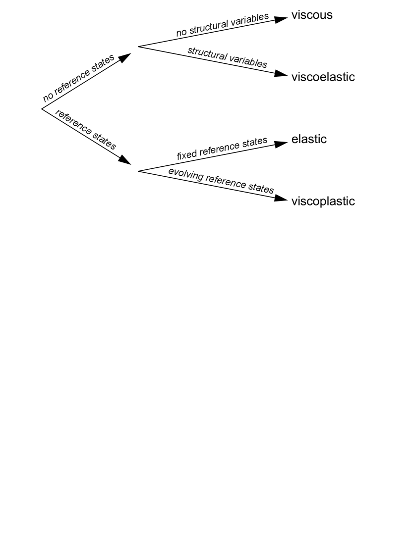
Figure 1: Attributes of rheological models.

The ideas of this paper naturally lead to a classification of rheological models, depending on whether or not we make use of reference states (see Fig. 1). From an abstract point of view, reference states occur when the Lie group providing the structure required to set up thermodynamics is not simply connected so that it can be written as the quotient of the universal covering group and a discrete group of reference states. In particular, we obtain a clear distinction between viscoplasticity and viscoelasticity, which often is not very transparent in the literature, in terms of reference states. In the absence of reference states we obtain the models of viscoelasticity which have been applied successfully to many complex fluids. The possibility of transitions between equivalent reference states is the hallmark of viscoplasticity.

Viscoplasticity is often defined as rate-dependent plasticity, where plasticity generally means the ability to change or deform permanently (in contrast to elasticity, which refers to the ability to change temporarily and revert back to the original form). These permanent changes occur by transitions from reference states to equivalent ones. Within the domain of a particular reference state, deformations are reversible and hence elastic. Only when a sufficiently high stress level is reached, transitions between equivalent reference states occur with a noticeable rate (in principle, transitions are possible even in the absence of stresses, but they are extraordinarily rare). This stress level is known as the yield point or, for anisotropic materials, as the yield surface. As yield is a matter of “noticeability,” phenomenological definitions of viscoplasticity based on this concept may not be ideal. The deformation behavior described by long-living reference states is often referred to a elastic-viscoplastic, whereas transitions at a noticeable rate lead to a plastic flow associated with a very large viscosity.

The deformation with respect to evolving reference states enters many models of viscoplasticity in which the total deformation is split into a plastic and an elastic part, where only the elastic part is used as a structural variable (see Leonov [14], Hütter and Tervoort [11] and references therein). Such a splitting corresponds directly to the factorization of a covering group. Usually, the relative or elastic deformation is treated by explicit variables, whereas the transition rate between reference states merely contributes to the rate of change of the relative deformation variable. The relative deformation measures used in previous phenomenological models of viscoplasticity correspond to moments of the configurational distribution function in the kinetic theory of the present paper, just as the conformation tensors of the Maxwell and Oldroyd models of viscoelasticity correspond to second moments of the connector vector of a Hookean dumbbell model in polymer kinetic theory [2]. Even if a kinetic theory on the quotient group does not treat reference states explicitly, the suggested analysis of the group theoretical background clearly shows the underlying existence of reference states and hence the viscoplastic nature of the models. Group theory thus helps to identify viscoplastic models, and the phenomena described by such models in a meaningful way are then recognized as viscoplastic.

Kinetic theories of viscoplasticity, such as the toy model employed for the purpose of illustration, are a promising starting point for deriving existing phenomenological models and for generalizing them, both for crystalline and for amorphous materials. They offer a link between detailed atomistic considerations [4, 1, 12] and phenomenological models [24, 22, 3]. For deriving kinetic theories by statistical mechanics [19, 17, 18, 20], it is important to realize the occurrence of discrete sets of reference states and of transition rates. The statistical mechanics of models with reference states should hence be expected to be based on Kramers-type formulas [13] for transition rates.

References

- Arsenlis et al. [2004] Arsenlis, A., Parks, D. M., Becker, R., Bulatov, V. V., 2004. On the evolution of crystallographic dislocation density in non-homogeneously deforming crystals. J. Mech. Phys. Solids 52, 1213–1246.
- Bird et al. [1987] Bird, R. B., Curtiss, C. F., Armstrong, R. C., Hassager, O., 1987. Kinetic Theory, 2nd Edition. Vol. 2 of Dynamics of Polymeric Liquids. Wiley, New York.
- Boyce et al. [1988] Boyce, M. C., Parks, D. M., Argon, A. S., 1988. Large inelastic deformation of glassy polymers. Part I: Rate dependent constitutive model. Mech. Mater. 7, 15–33.
- El-Azab [2000] El-Azab, A., 2000. Statistical mechanics treatment of the evolution of dislocation distributions in single cystals. Phys. Rev. B 61, 11956–11966.
- Eyring [1936] Eyring, H., 1936. Viscosity, plasticity, and diffusion as examples of absolute reaction rates. J. Chem. Phys. 4, 283–291.
- Gardiner [1990] Gardiner, C. W., 1990. Handbook of Stochastic Methods for Physics, Chemistry and the Natural Sciences, 2nd Edition. Springer Series in Synergetics, Volume 13. Springer, Berlin.
- Grmela and Öttinger [1997] Grmela, M., Öttinger, H. C., 1997. Dynamics and thermodynamics of complex fluids. I. Development of a general formalism. Phys. Rev. E 56, 6620–6632.
- Hamermesh [1989] Hamermesh, M., 1989. Group Theory and its Application to Physical Problems. Dover, New York.
- Hütter [2009] Hütter, M., 2009. Tensorial Orowan equation, the driving force for viscoplastic deformation, and the relation to the Peach-Koehler force. J. Mech. Phys. Solids ??, submitted.
- Hütter et al. [2009] Hütter, M., Grmela, M., Öttinger, H. C., 2009. What is behind the plastic strain rate? Rheol. Acta 48, 769–778.
- Hütter and Tervoort [2008] Hütter, M., Tervoort, T. A., 2008. Thermodynamic considerations on non-isothermal finite anisotropic elasto-viscoplasticity. J. Non-Newtonian Fluid Mech. 152, 53–65.
- Johnson et al. [2007] Johnson, W. L., Demetriou, M. D., Harmon, J. S., Lind, M. L., Samwer, K., 2007. Rheology and ultrasonic properties of metallic glass-forming liquids: A potential energy landscape perspective. MRS Bulletin 32, 644–650.
- Kramers [1940] Kramers, H. A., 1940. Brownian motion in a field of force and the diffusion model of chemical reactions. Physica 7, 284–304.
- Leonov [1976] Leonov, A. I., 1976. Nonequilibrium thermodynamics and rheology of viscoelastic polymer media. Rheol. Acta 15, 85–98.
- Marsden and Ratiu [1999] Marsden, J. E., Ratiu, T. S., 1999. Introduction to Mechanics and Symmetry, 2nd Edition. Texts in Applied Mathematics, Volume 17. Springer, New York.
- Öttinger [1996] Öttinger, H. C., 1996. Stochastic Processes in Polymeric Fluids: Tools and Examples for Developing Simulation Algorithms. Springer, Berlin.
- Öttinger [1998] Öttinger, H. C., 1998. General projection operator formalism for the dynamics and thermodynamics of complex fluids. Phys. Rev. E 57, 1416–1420.
- Öttinger [2000] Öttinger, H. C., 2000. Derivation of two-generator framework of nonequilibrium thermodynamics for quantum systems. Phys. Rev. E 62, 4720–4724.
- Öttinger [2005] Öttinger, H. C., 2005. Beyond Equilibrium Thermodynamics. Wiley, Hoboken.
- Öttinger [2007] Öttinger, H. C., 2007. Systematic coarse graining: ‘Four lessons and a caveat’ from nonequilibrium statistical mechanics. MRS Bulletin 32, 936–940.
- Öttinger and Grmela [1997] Öttinger, H. C., Grmela, M., 1997. Dynamics and thermodynamics of complex fluids. II. Illustrations of a general formalism. Phys. Rev. E 56, 6633–6655.
- Pan and Rice [1983] Pan, J., Rice, J. R., 1983. Rate sensitivity of plastic flow and implications for yield-surface vertices. Int. J. Solids Struct. 19, 973–987.
- Ree and Eyring [1955] Ree, T., Eyring, H., 1955. Theory of non-newtonian flow. I. Solid plastic systems. J. Appl. Phys. 26, 793–800.
- Rice [1971] Rice, J. R., 1971. Inelastic constitutive relations for solids: An internal-variable theory and its application to metal plasticity. J. Mech. Phys. Solids 19, 433–455.
- Rossmann [2002] Rossmann, W., 2002. Lie Groups: An Introduction Through Linear Groups. Oxford Graduate Texts in Mathematics, Volume 5. Oxford University Press, Oxford.
- Salmon [1988] Salmon, R., 1988. Hamiltonian fluid mechanics. Annu. Rev. Fluid Mech. 20, 225–256.