AROMA: Automatic Generation of Radio Maps for Localization Systems

Abstract

WLAN localization has become an active research field in recent years. Due to the wide WLAN deployment, WLAN localization provides ubiquitous coverage and adds to the value of the wireless network by providing the location of its users without using any additional hardware. However, WLAN localization systems usually require constructing a radio map, which is a major barrier of WLAN localization systems’ deployment. The radio map stores information about the signal strength from different signal strength streams at selected locations in the site of interest. Typical construction of a radio map involves measurements and calibrations making it a tedious and time-consuming operation.

In this paper, we present the design, implementation, and evaluation of the AROMA system that automatically constructs accurate active and passive radio maps for both device-based and device-free WLAN localization systems. AROMA has three main goals: high accuracy, low computational requirements, and minimum user overhead. To achieve high accuracy, AROMA uses 3D ray tracing enhanced with the uniform theory of diffraction (UTD) to model the electric field behavior and the human shadowing effect. AROMA also automates a number of routine tasks, such as importing building models and automatic sampling of the area of interest, to reduce the user’s overhead. Finally, AROMA uses a number of optimization techniques to reduce the computational requirements.

We present our system architecture and describe the details of its different components that allow AROMA to achieve its goals. We evaluate AROMA in two different testbeds. Our experiments show that the predicted signal strength differs from the measurements by a maximum average absolute error of 3.18 dBm achieving a maximum localization error of 2.44m for both the device-based and device-free cases. Our results also show that ignoring the effect of the UTD in the device-free case leads to significant degradation in accuracy up to more than 700%. We also relay lessons learned and give directions for future work.

1 Introduction

WLANs are installed primarily for providing wireless communications. However, recent research has shown that WLANs can be used in location determination in indoor environments, without using any extra hardware [3, 19, 26, 25, 13, 24]. Acquiring the location information for a tracked entity unleashes the possibility of various context-aware applications including location-aware information retrieval, indoor direction finding, and intrusion detection.

There are two classes of WLAN location determination systems: device-based, e.g. [3, 25] and device-free, e.g. [24, 13]. Device-based systems track the location of a WLAN-enabled device, such as a laptop or PDA. On the other hand, device-free systems do not require the entity being tracked to carry a device and depend on analyzing the effect of the tracked entity on the signal strength to estimate the entity’s position. Device-free localization systems are composed of a number of access points (APs) and monitoring points (MPs). The MPs, such as standard laptops and other wireless-enabled devices, monitor the APs signal strengths and have fixed locations.

Both device-based and device-free systems usually work in two phases: an offline training phase and an online location determination phase. During the offline phase, the system collects signal strengths received from different streams at different selected locations in the area of interest, and tabulates them into a so-called radio map. For device-based systems, each stream represents the signal strength from an AP to the tracked device. For device-free systems, each stream represents an (AP, MP) pair and the radio map tabulates the effect of the tracked entity on the fixed streams. The difference between active and passive radio maps’ construction is illustrated in Figure 1.

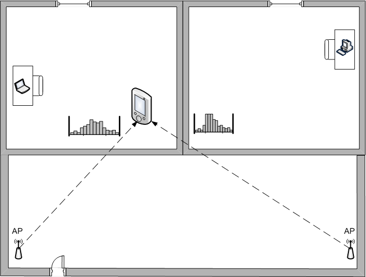
(a) Active

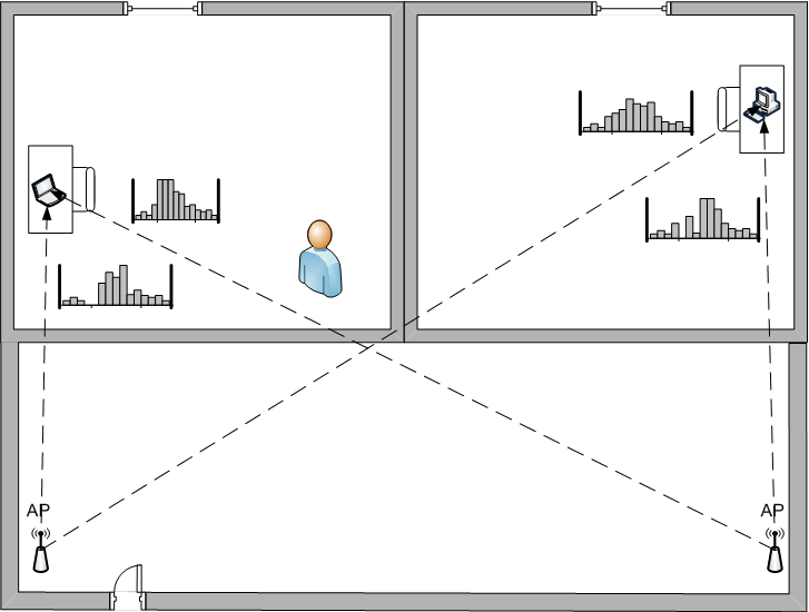
(b) Passive

Figure 1: Difference between active and passive radio maps construction. In a passive radio map, we have a histogram per raw data stream, as compared to a histogram per AP. Also, a user does not carry any device when constructing the passive radio map.

During the location determination phase, the system uses the information stored in the radio map to estimate the user’s location. Different location determination systems store different information in the radio map. For example, the Horus system [25] stores the signal strength distribution of the signal strength received from each AP, while the Radar system [3] stores the average signal strength received from each AP.

Current methods of radio maps’ construction use manual calibrations making it a tedious and time-consuming operation. Furthermore, each time the layout of the environment changes or different hardware is used, the whole process of constructing the radio map has to be repeated. In addition, the process of radio map construction gets more complicated, in the device-free case, when the number of tracked entities increases, since the radio map needs to take all the combination of the possible tracked entities’ locations into account. For example, for a radio map with $l$ locations and a system that wants to track up to $n$ entities, the radio map needs to store information about $l\choose n$ possibilities. This emphasizes the need for a method to automatically construct the radio maps for an area of interest.

In this paper we present the AROMA (Automatic generation of RadiO MAps) system which can automatically construct an accurate radio map for a given 3D area of interest. AROMA is unique in supporting automatic radio map generation for both device-based and device-free localization systems. To our knowledge, AROMA is the first system to consider radio map generation for device-free systems and the first to consider human effects in device-based systems. AROMA combines ray tracing with the uniform theory of diffraction [14] to model both the RF propagation and human shadowing effect. Ray tracing approximates the electromagnetic waves as a set of discrete ray tubes that propagate through the area of interest and that undergo attenuation, reflection, transmission and diffraction due to the complexity of an indoor environment. Although ray tracing has been used before in site-specific radio propagation prediction and several tools have been developed, e.g. [20, 22, 2, 12, 23], the main focus of such tools was the radio coverage problem, i.e. determining the coverage holes given the APs’ positions. This does not require high accuracy, and therefore, none of these tools account for the human shadowing effect on the RF signal. Existing papers on the human shadowing effect, e.g. [7], illustrate only the theory behind the modeling and not its application. On the other hand, propagation modeling for localization systems requires high accuracy, where variations in the predicted signal strength can lead to large localization errors. Therefore, the AROMA system has three main goals: (1) to automatically construct an accurate radio map for a site of interest, (2) to have efficient computations, and (3) to incur minimum overhead on the user.

We present the design of the AROMA system and give details about its different components and how they interact to achieve its goals. We also evaluate the system under two testbeds for the device-based and device-free cases.

The rest of the paper is organized as follows. Section 2 presents the details of the AROMA system. We evaluate the performance of the system under two different testbeds in Section 3. We discuss our experience while building the system in Section 4. In Section 5 we discuss related work. Finally, Section 6 concludes the paper and gives directions for future work.

2 The AROMA System

2.1 Overview

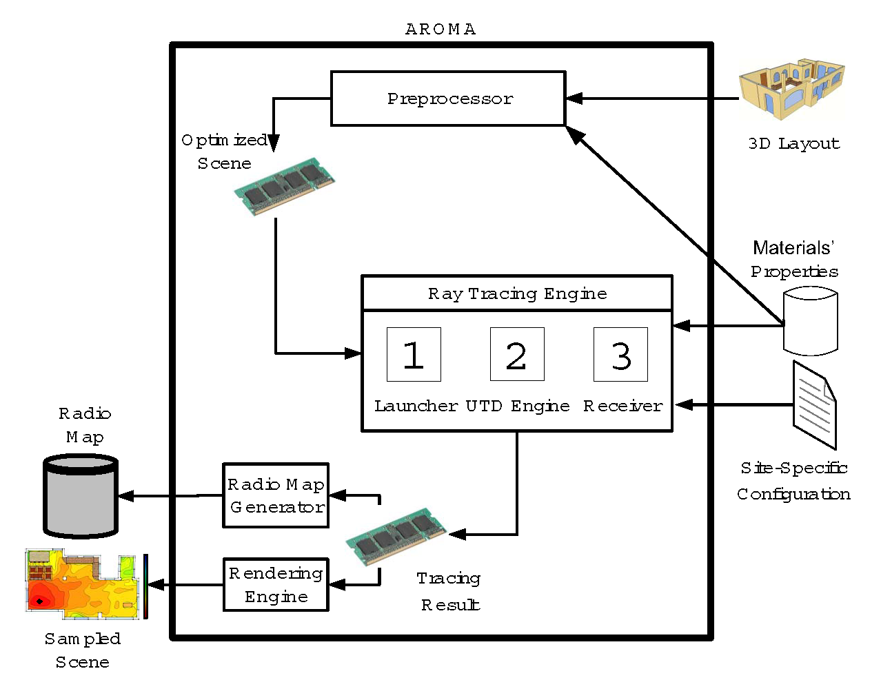
Figure 2: AROMA system architecture.

The AROMA System uses site-specific ray tracing, augmented with the uniform theory of diffraction (UTD), to predict the RF propagation in a 3D site. Figure 2 shows the architecture of the AROMA System. The input to AROMA is the 3D model of the site of interest which can be imported automatically from CAD tools or drawn using any free 3D modeling tool found in the market today such as Google SketchUp and Blender. The 3D manipulation of the site model is done using the jMonkeyEngine (jME) [18] which is a high performance open-source Java-based gaming engine.

Besides the 3D model, the user must provide the site-specific configuration. This includes the locations and antenna characteristics of the APs and MPs. The antenna characteristics include transmitting power, frequency, maximum gain and radiation pattern. The system comes with two pre-defined antenna radiation patterns: isotropic and half-wave dipole antenna. The user can also define a customized radiation pattern depending on the hardware used. The user has two options to specify the site-specific configuration:

1. Insert them manually using the UI tool.

2. Provide a configuration file with their locations and antenna characteristics.

The user has similar options when specifying the locations of the radio map cells.

AROMA comes with a built-in DB of the approximate values of the RF propagation properties of common building materials such as bricks and concrete. The user has the options of using this DB or providing customized values using the UI tool.

After providing the 3D model and the site-specific configuration, the user starts the system. The 3D model is first pre-processed to extract the edges in the scene. The Ray Tracing Engine is the core of the AROMA system and is composed of three modules: the Ray Launcher, the UTD Engine, and the Ray Receiver. The Ray Launcher samples the electromagnetic waves emitted from the the APs into a set of discrete ray tubes covering the area of interest uniformly and each having an associated electric field. The ray tubes propagate into the environment and undergo reflections, transmissions and diffractions. The Ray Tracing Engine handles the interactions of the ray tubes with the environment. The UTD Engine handles the changes in the electric field associated with the ray tubes resulting from these interactions. The contribution of each tube in the final received signal strength at the MPs can be found by the Ray Receiver. The tracing result is then processed by the Radio Map Generator to generate the radio map. A sampled scene with RF prediction levels rendered on its floor can also be generated by processing the tracing result by the Rendering Engine. The overall algorithm used in the AROMA system is briefed in Algorithm 1. Each component is explained in details in the next subsections.

Algorithm 1 Ray Tracer algorithm

  start preprocessing;

  for all access point AP do

     Queue $Q\leftarrow launchRays()$;

     for $i=1$ to depth step 1 do

        while $\neg empty(Q)$ do

           $ray\leftarrow dequeue(Q)$;

           $event\leftarrow interaction(ray,site)$;

           $process(event)$;

           $utd(event)$;

           if $receivable(receiver,ray)$ then

              $receive(receiver,ray)$;

           end if

        end while

     end for

  end for

  start postprocessing;

2.2 Pre-Processing

The pre-processor works on the 3D model to extract edges in the model and to assign different materials to the faces in the model. In addition it constructs data structures that helps in speeding up the computations.

2.2.1 Edge Detection

The 3D model is loaded in the tool as an array of tri-meshes. A tri-mesh is a set of triangles covering possibly non-contiguous surfaces. An edge in the model can be spread over multiple tri-meshes, which need to be merged for accurate modeling of wedge diffraction and for efficient computations. The edge detection module uses the hysteresis algorithm [1] to detect the edges in the 3D model. The algorithm consists of two phases. During the classification phase, each triangle side is assigned a weight which is the largest angle between the normals to any two adjacent triangles sharing that side. In the detection phase, a triangle side is considered an edge if it passes the hysteresis test, where two thresholds are defined. If the weight of the side is greater than the upper threshold, then the side is considered an edge. If it is lower than the lower threshold, the side is discarded. Other sides are considered edges if they neighbors an edge.

2.2.2 Bounding Capsules

The pre-processor encapsulates edges and wedges by bounding capsules (a swept sphere containing the object) and assigns them unique IDs to efficiently test for ray-edge intersection events. Bounding capsules has an advantage over bounding cylinders as a capsule and another object intersect if the distance between the capsule’s defining segment and some feature of the other object is smaller than the capsule’s radius [21]. Bounding capsules are also used to calculate intersections with the human bodies in the environment and to efficiently diffract rays around them.

2.2.3 Materials Detection

To handle different materials efficiently, the pre-processor assigns all edges that have the same material the same color. This makes the 3D model more efficient for processing by the jMonkeyEngine.

2.3 Ray Tracing Engine

2.3.1 Ray Launcher

APs are represented as point sources that emit electromagnetic waves having spherical wavefronts. These spherical wavefronts are divided into a number of ray tubes that cover them entirely and have equal area. Each ray tube is represented by a ray located at its center. The rays emitted from each AP must experience two forms of uniformity [6]:

1. Large scale uniformity: to guarantee unbiased coverage of rays in the 3D environment,

2. Small scale uniformity: to guarantee that the angular separation between rays is constant.

These conditions are satisfied by emitting rays through the vertices of an icosahedron whose center is the transmitter. An icosahedron has 12 vertices and the angular separation between rays emitted from its vertices equals $69^{\circ}$. To achieve a better angular resolution, the face of the icosahedron is divided into smaller triangles using a tessellation frequency N [20]. The rays are then emitted from the vertices of the formed triangles and the ray tubes are hexagonal in shape as shown in Figure 3. A good approximation for the angular separation between rays in this case is [6]:

$$\alpha=\frac{69.0{}^{\circ}}{N}$$ (1)

Section 4.4 discusses the values used for the ray tracing parameters.

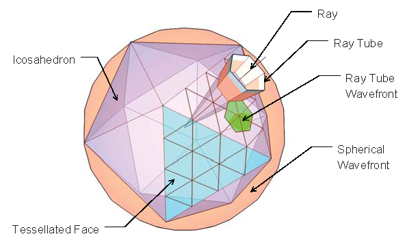
Figure 3: Ray launching by tessellating the faces of an icosahedron. The transmitter is located at the center of the icosahedron. Each icosahedron face is tessellated into smaller triangles using a tessellation frequency (N). Rays are launched passing through the vertices of the produced triangles.

2.3.2 Ray Tracer

The complex indoor environment causes the ray tubes to change their original direction through either reflection, transmission, or diffraction. This results in a phenomena known as multipath fading where the transmitted signal reaches a receiver via multiple paths.

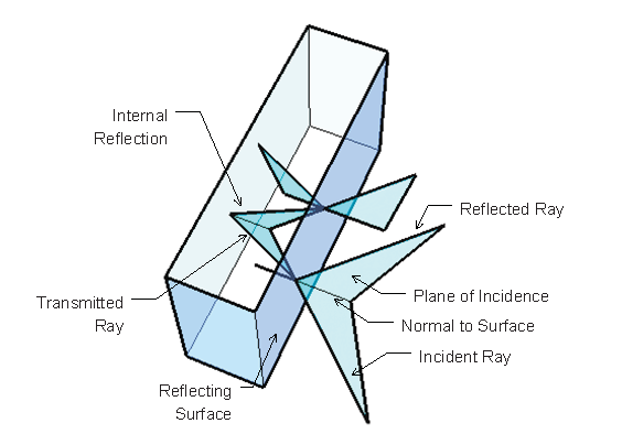
Figure 4: Reflection and transmission of rays. A ray incident on a surface experiences reflection and transmission. The transmitted ray suffers also from internal reflection and transmission.

Each ray is traced for different kinds of interactions with the 3D site. A ray incident on an object produces a reflected and a transmitted rays as shown in Figure 4. Reflected rays satisfy the laws of reflection:

1. The incident ray, reflected ray, and the normal to the reflecting surface are coplanar.

2. Angle of incidence equals the angle of reflection.

And the transmitted rays satisfy the laws of refraction:

1. The incident ray, refracted ray, and the normal to the reflecting surface are coplanar.

2. The ratio of the sines of the angles of incidence and refraction is equivalent to the opposite ratio of the indices of refraction (Snell’s Law).

   $$\frac{\sin\theta{}_{1}}{\sin\theta{}_{2}}=\frac{n{}_{2}}{n{}_{1}}$$ (2)

Where $\theta{}_{1}$ is the angle of incidence, $\theta{}_{2}$ is the angle of refraction, $n{}_{1}$ and $n{}_{2}$ are the refractive indices of the first and second mediums respectively.

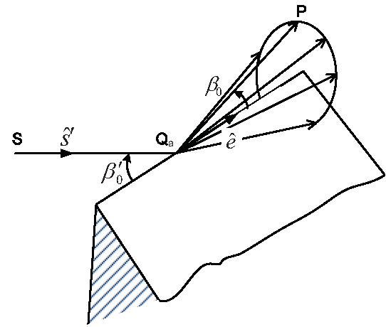
Figure 5: Wedge diffracion. A ray intersecting with an edge produces a set of diffracted rays forming a diffraction cone. $\beta_{0}$ is the angle between the incident ray and the edge, ${\hat{s}}^{{}^{\prime}}$ is the direction of the incident ray, $\hat{e}$ is the direction of the edge, and $\hat{s}$ is the direction of the diffracted ray. ${Q_{a}}$ is the point of intersection, and $P$ is any point in the space lying on the produced cone.

A ray incident on an edge produces a set of diffracted rays forming what is called a diffraction cone (as shown in Figure 5) obeying the law of diffraction:

A diffracted ray and the corresponding incident ray make equal angles with the edge at the point of diffraction, and they lie on opposite sides of the plane normal to the edge at the point of diffraction.

$$\sin{\beta}_{0}=|{\hat{s}}^{{}^{\prime}}\times\hat{e}|=|\hat{s}\times\hat{e}|$$ (3)

Where $\beta_{0}$ is the angle between the incident ray and the edge, ${\hat{s}}^{{}^{\prime}}$ is the direction of the incident ray, $\hat{e}$ is the direction of the edge, and $\hat{s}$ is the direction of the diffracted ray.

Each time the ray makes an interaction with the environment, its depth is incremented. The tracing of a ray ends in one of two cases:

1. The depth reaches a maximum user-defined value.

2. The power associated with the ray decreases below a defined minimum value.

2.3.3 UTD Engine

Electromagnetic waves are discretized using Geometrical Optics (GO) into a set of ray tubes. Each ray tube propagates in a direction identified by the ray located at its center, and has associated electric and magnetic fields orthogonal to each other and to the direction of propagation. GO can account for reflection and transmission [14]. The reflected and transmitted electric fields are related to the incident electric field using Fresnel’s Field Coefficients [4]. However, GO fails to account for the electric fields in the shadow regions which occur due to electric field diffraction. UTD addressed the GO deficiency which predicts zero electric field in human shadowed regions, and thus UTD is used in modeling wedge diffraction. Another reason for using UTD is that it overcomes the drawbacks of the Geometrical Theory of Diffraction (GTD), which is an extension of geometrical optics that accounts for diffraction [11]. GTD suffers from some problems [14], the most serious of them is that GTD predicts singular electric fields near the transition regions. In UTD, The diffracted electric field is related to the incident electric field using UTD diffraction coefficients [14].

The construction of device-free radio maps requires modeling of human’s body effect on RF signals. At microwave frequencies and higher, the human body constitutes an impassable reflector for electromagnetic waves. That is, incident waves are reflected and diffracted off the body, along other interactions with the surrounding environment. Previous work in human modeling has shown a strong correlation between the RF characteristics of the human body and a metallic circular cylinder [7] in indoor radio channels. Therefore, we use a metallic cylinder to model the human body with radius $0.15m$, and height $2m$ [7].

All equations related to the UTD Engine are illustrated in Appendix A.

2.3.4 Ray Receiver

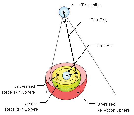
Figure 6: Reception sphere. The size of the reception sphere should be large enough to intersect only one ray from a given wavefront.

MPs are represented as point sinks. A ray is received if the MP lies within its ray tube. Alternatively, and for efficiency, we can consider a ray received if it lies within a certain distance from the MP. This distance depends on the size of the ray tube at the MP. The reception sphere model is based on this observation [20]. A sphere is formed around the MP such that at most one ray from a wavefront intersects with the sphere, as illustrated in Figure 6. The reception sphere radius equals to the radius of the circle circumscribed about the hexagonal wavefront of the ray tube. Different rays have different reception sphere radii calculated as:

$$r=\ \frac{\alpha\ l}{\sqrt{3}}$$ (4)

Where $\alpha$ is the angular separation between rays and $l$ is the total unfolded distance traveled by the ray till the perpendicular projection of the receiver on the ray path.

2.4 Post-Processing

2.4.1 Radio Map Generator

A radio map is constructed by dividing the area of interest into a number of locations, each location has a corresponding cell in the radio map. The user should provide a list of the radio map cell locations and the required type of radio map, i.e. active or passive radio map (Figure 1). As another option, the user can select a radio map spacing and the system can automatically generate the radio map locations.

2.4.2 Rendering Engine

The tracer can sample the site area to predict the signal strength across the entire site of interest. The tracing result are then color-shaded and layered over the site floor by the Rendering Engine. At the sampling step, an isotropic antenna is virtually positioned at each sampling point and the overall sampling result is then bi-cubically interpolated over the whole floor area (Figure 7).

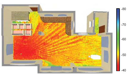
Figure 7: An example of the output of the rendering engine. At the sampling step, an isotropic antenna is virtually positioned at each sampling point and the overall sampling result is then bi-cubically interpolated over the whole floor area.

3 System Evaluation

Our validation is composed of two experiments: one for the device-based radio map generation and the other for the device-free radio map generation. We used two Cisco Aironet 1130G Series 802.11G Access Point and two D-Link DWL-G650 NICs. The system is currently implemented in the Windows OS. A NIC Query[15] driver that provides an API for user-level queries of NDIS[16] devices is used to collect the signal strength samples. We collected 60 samples for each location in each experiment. Each experiment has different configurations that will be illustrated in details in the next subsections.

3.1 Device-based Radio Map Generation

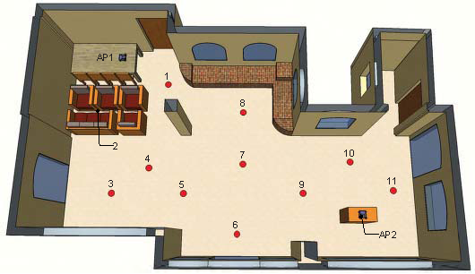
Figure 8: Device-based experiment layout. The figure highlights the locations of APs and radio map locations.

The experiment was conducted in a typical apartment with an area of $700{ft}^{2}$. The environment contains furniture and is composed of different materials, like bricks, concrete, wood and glass. We marked 11 different locations covering the entire area as shown in Figure 8. The APs’ configurations are summarized in Table 1.

$P_{t}$	$2mW$
$Antennagain(G_{max})$	$3.0dBi$
$Frequency(f)$	$2.4GHz$
Antenna Type	Isotropic

Table 1: APs’ configurations for the device-based experiment.

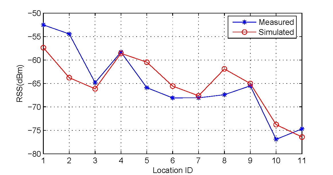
(a) RSS from AP1

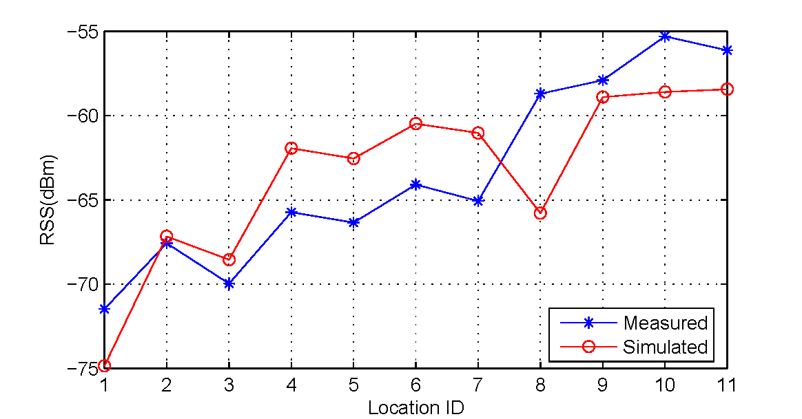
(b) RSS from AP2

Figure 9: Device-based experiment, measured vs. simulated RSS. Location ID refers to the IDs in Figure 8.

Figure 9 shows the simulated and measured values for the two APs. Table 2 summarizes the results. The figure shows that the tool gives the same trend as the measurements with a maximum average absolute error of less than 3.2 dBm for the two APs. This shows that the tool can be used to model more complex scenarios of behavior in a device-based setting.

3.2 Device-free Radio Map Generation

The experiment was held in the same environment as that of the device-based radio map experiment. 44 locations were chosen and are illustrated in Figure 10. A new location is introduced here, namely location 0, which represents the environment without the human. The APs’ configurations are summarized in Table 1.

Figure 11 shows the simulated versus measured RSS for the experiment. The results are summarized in Table 3. The results show that simulated values are close to the measured values with a maximum average absolute error of 2.17 dBm for all streams. The figure also shows that the human effect is maximum when the person is cutting the line-of-sight, e.g. locations 11, 34, and 35 in Figure 11(d). This is captured by both the tool and the actual measurements which shows that the tool can be used to model more complex scenarios of behavior in a device-free setting.

	AP1	AP2
RMSE	4.00 dBm	3.4 dBm
Average absolute error	3.2 dBm	3.1 dBm
Standard deviation	3.18	3.10

Table 2: Device-based experiment, measured vs. simulated results.

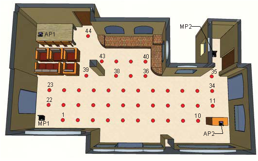
Figure 10: Device-free experiment layout. The figure highlights the locations of APs, MPs, and radio map locations.

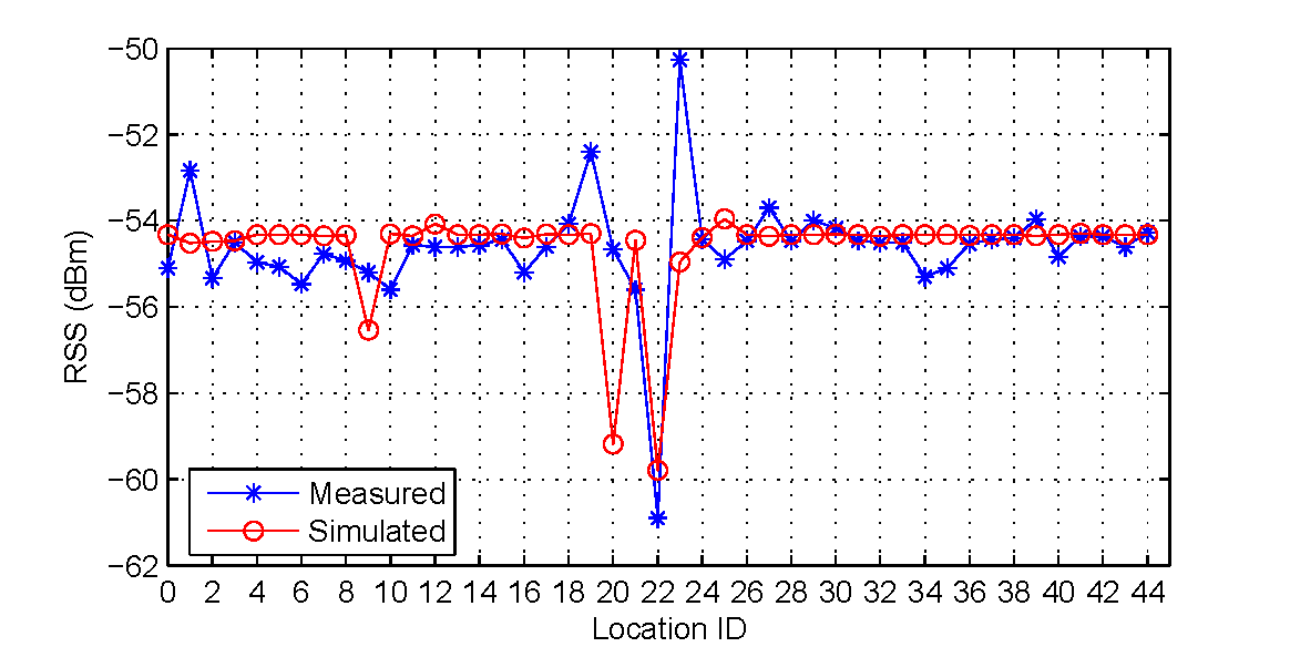
(a) RSS from AP1 by MP1

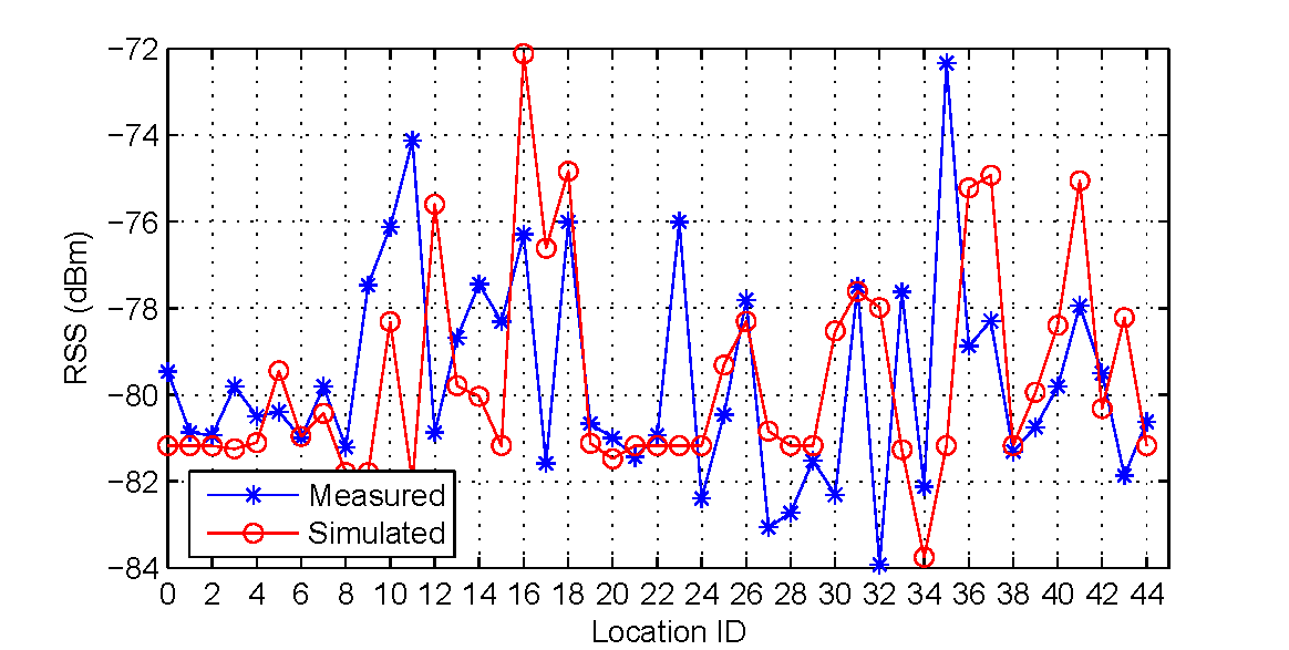
(b) RSS from AP1 by MP2

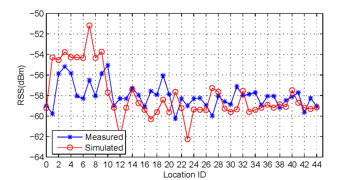
(c) RSS from AP2 by MP1

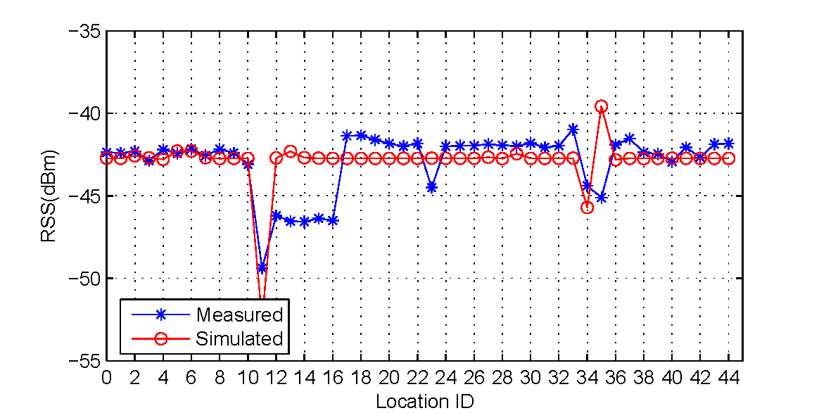
(d) RSS from AP2 by MP2

Figure 11: Device-free experiment, measured vs. simulated RSS. Location ID refers to the IDs in Figure 10.

		AP1	AP2
MP1	RMSE	1.19 dBm	2.11 dBm
	Avg. Abs. Err.	0.71 dBm	1.61 dBm
	Stdev	1.2	2.13
MP2	RMSE	3.02	1.75
	Avg. Abs. Err.	2.17 dBm	1.21 dBm
	Stdev	3.06	1.77

Table 3: Device-free experiment, measured vs. simulated results.

3.3 Localization Performance

In this section, we compare the performance of a simple nearest-neighbor localization classifier, similar to the Radar system [3], when trained by measured and simulated data. We divide the collected samples into two parts with a ratio of 2 to 1. The larger part is used as a training data for the measurements-based classifier and the other as a testing data for both types of classifiers.

The results are summarized in Table 4. For the device-based localization system, the mean distance error calculated for the measurement-based and simulation-based classifiers are 0.89m and 1.61m respectively. Similarly, for the device-free case, the mean distance error calculated for the measurement-based and simulation-based classifiers are 0.96m and 2.44m respectively. Note that since cross-validation is used to evaluate the measurement-based classifier, its accuracy is over estimated. Using an independent test set, the accuracy of the measurement-based classifier will be worse, while the accuracy of the simulation-based classifier will not be affected. Therefore, the difference between the measurement-based and simulation-based classifiers will be less.

Radio map	Measurements-based Classifier	Simulation-based Classifier
Device-based	$0.89m$	$1.61m$
Device-free	$0.96m$	$2.44m$

Table 4: Localization performance (mean distance error) for the device-based and device-free experiments.

3.4 Effect of Ignoring the UTD

In this section, we show the effect of not using the UTD engine, which is the common practice in previous work in the area of RF propagation. Turning off the UTD engine disables all the interaction with the human except for the attenuation effect, i.e. the signal is attenuated by a constant amount if the human is obstructing the signal. Figure 12 shows the results and Table 5 summarizes them. The results show that ignoring the contribution of the UTD engine degrades the performance significantly, up to 706%. This is specially true for MP2, where its location makes it significantly affected by the UTD effects (Figure 10).

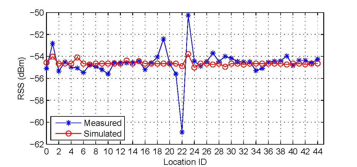
(a) RSS from AP1 by MP1

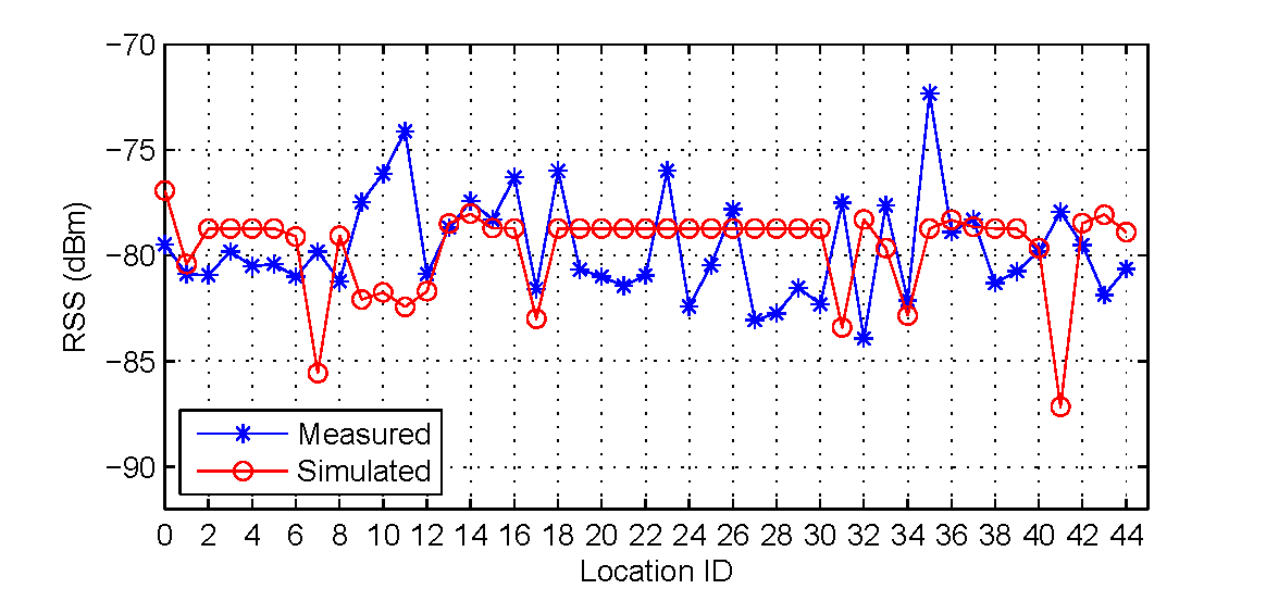
(b) RSS from AP1 by MP2

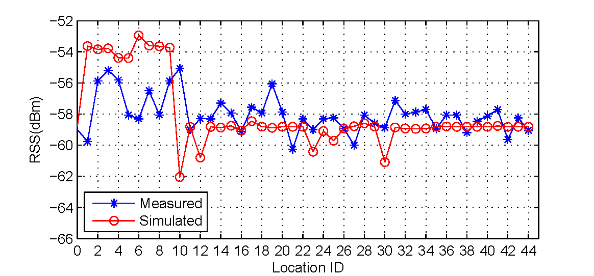
(c) RSS from AP2 by MP1

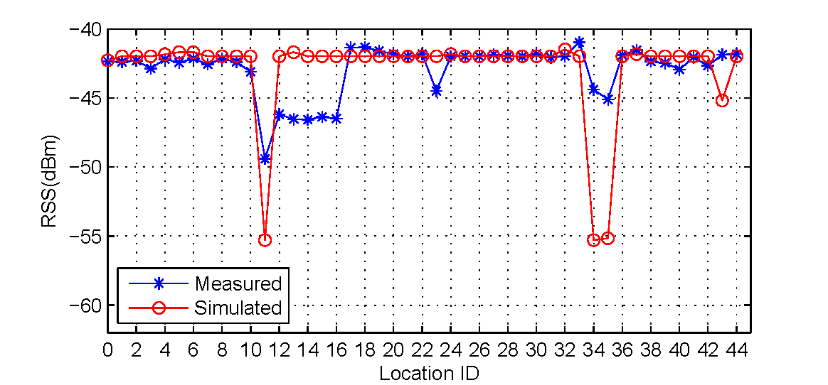
(d) RSS from AP2 by MP2

Figure 12: Device-free experiment when the UTD engine is not used, measured vs. simulated RSS.

4 Discussion

In this section, we discuss different aspects of the AROMA system and our experience while developing it.

4.1 Computational Efficiency

The AROMA system uses a number of techniques to reduce the computational overhead of ray tracing. Using bounding capsules, combining edges, and mapping materials to colors are all performed at the pre-processing stage to increase the efficiency of different modules while the ray tracing engine is running. In addition, the ray launcher’s parameters can be tuned for maximum accuracy and performance. Finally, the concept of reception sphere is used in the ray receiver to further reduce computational requirements.

4.2 Ease of Use

Our AROMA system contains a number of modules that enhance the user experience and automate common tasks. The UI module allows the user to use point-and-click to enter the locations of APs and MPs. Different wizards are provided for the user to enter the APs and MPs parameters, e.g. the antenna’s pattern, and materials properties. A database of different materials’ properties, along with a set of predefined antenna patterns are also included to reduce the overhead of entering this information. In addition, the user can configure the system to automatically select the radio map locations.

4.3 Prediction Precision

In a perfect world, the measured RSS should match the predicted RSS perfectly. There are different reasons for deviation of the predicted values from the measured ones. Extensive work has been done in the characterization of signal loss for various materials in indoor environments. However, in practice the physical and electrical characteristics of materials vary considerably from theory. This variance affects greatly the accuracy of signal prediction. In a similar manner, the human body is made up of water that causes the signal to attenuate. The amount of signal loss depends on the size of a human body and its orientation that varies considerably from one person to another.

In addition, there are always discrepancies between hardware characteristics and the characteristics included in its data sheet. The effect of these discrepancies is inevitable. The most influencing discrepancy is that resulting from the antennas radiation patterns and orientation. The difference between where the radio point location is selected and where the human is actually standing is another reason for deviation. In summary, the reasons of deviation of predicted values from the measurements include:

• Lacking of a perfect 3D model of the environment.

• Lacking of the precise electrical characteristics of the materials in the environment.

• Hardware discrepancies.

• UTD assumes diffraction off perfect conductors, yet the environment contains diverse dielectrics.

• Surrounding noise and imprecise human location.

		AP1	AP2
MP1	RMSE	2.87 dBm	5.91 dBm
	Avg. Abs. Err.	2.60 dBm	5.49 dBm
	% degradation	266%	241%
	Stdev	1.22	2.20
MP2	RMSE	11.53 dBm	10.19 dBm
	Avg. Abs. Err.	11.01 dBm	9.76 dBm
	% degradation	407%	706%
	Stdev	3.46	2.95

Table 5: Device-free experiment when the UTD engine is not used, measured vs. simulated results.

4.4 Ray Tracing Parameters

The ray tracing algorithm has two parameters namely: tessellation frequency of APs ($N$) and tracing depth ($d$). Throughout our experiments, we noticed that the results are not sensitive to the tracing depth. The reason behind this is that rays at higher depths have smaller power and thus make little contribution to the received signal. We used a tracing depth of 4 in our experiment. A tessellation frequency between 4 and 8 gives both good accuracy and efficient computations.

4.5 Radio Maps for Probabilistic Localization Systems

The localization results reported in this paper are for deterministic location determination systems that depend on storing the average RSS in the radio map. Probabilistic location determination systems, e.g. [25], store RSS distributions in the radio map. In order to generate a probability distribution, different approaches can be used: Perturbing the location of the device or human, for device-based and device-free systems respectively, leads to changing the generated radio map and hence can be used to estimate the probability distribution. Similarly, the locations and antenna patterns of APs and MPs and the state of doors and windows can be changed to achieve a similar effect. Another possibility is to develop models for the relation between the average RSS of a stream and its variance. Previous studies have reported that the higher the average RSS, the higher the variance [25]. This effect can be more accurately quantified and used.

4.6 Dynamic Radio Map Generation

The radio map can change also from time to time based on the environment conditions. To capture these changes, the antennas’ parameters and the building materials can be adjusted based on environment changes, such as temperature and/or humidity over the day or for a given semester in the year. Other effects that are dependent on the time of the day, such as human density, can also be included in the tool, e.g. by randomly placing humans in the area of interest based on the time of day.

Feeding the tool with a small number of tuning measurements from the environment can be used as another technique to change the system’s parameters to capture the changes in the environment.

4.7 Human Modeling

Currently, the AROMA system models the human as a perfectly conducting cylinder [7]. Although this gives good results, we believe that the system’s accuracy can be enhanced, especially for the device-free case, by having a better human model. The main drawback of the cylinder model is that it does not capture the effect of the user’s orientation. This is an area for ongoing work.

4.8 Other Uses

In this paper, we showed how the AROMA system can be used in constructing accurate radio maps for device-based and device-free localization systems. However, the AROMA system can also be used in a number of different applications. In addition to the traditional site planning, such as determining the placement of APs to maximize coverage and detect coverage holes, AROMA can be used to select the locations of APs and MPs for maximum combined coverage and localization accuracy. AROMA can be also used in the design of new algorithms for localization systems, especially for the challenging and open research area of device-free tracking and identification [24]. The system can be used to test the effect of the existence of different humans in the area on the constructed radio map and the effect of different instance of the same object. Another application for the system is in studying the effect of the new smart APs that have automatic power adjustment on the performance of localization systems.

5 Related Work

Indoor radio propagation has been an active field of research [20, 22, 2, 12, 23], especially for cellular networks. Seidel and Rappaport discuss different radio propagation models in [20]. Based on the ray-tracing technique, most authors model the propagation loss using the simple attenuation model:

$$P\left(d\right)=P\left(d_{0}\right)-10\times n\times{\log 10}\left(\frac{d}{d_{0}}\right)$$ (5)

Where $P\left(d\right)$ is the power at distance $d$ from the transmitter, $P\left(d_{0}\right)$ is the power at a reference distance, and $n(\geq 2)$ is the attenuation exponent.

The simple attenuation model requires extensive measurements in order to estimate a best-fit attenuation exponent that reduces the overall error for a certain site. In [9], Hills et al. report that an attenuation exponent of 2.60 results in the best fit in the buildings on the Carnegie Mellon University campus. Beside requiring extensive site-specific measurements to estimate its parameters, the model does not account for attenuation effects from typical environments, like doors, walls, and other different materials.

A more sophisticated model is the partition model. The partition model takes into consideration path loss caused by indoor partitions, like walls and doors. This simple model cannot give sufficient accuracy for localization systems. For example, the Radar system, which accounts for multiple wall attenuation effects along the direct path between transmitters and receivers, has a mean error of 3.4m [3]. As we show in Section 3 and Table 4, the AROMA system can give accuracy of 1.61 m in a similar environment. In addition, the proposed tools has a number of other uses as discussed in Section 4.

Another model that is closely related to the partition model is the site-specific model. The site-specific model behaves like the partition model, but it needs more site-specific parameters such as materials and geometrics. Ali et al. [8] introduced a novel model that relate the average path power to the site-specific parameters. However, such systems do not consider the human effect and their goal is to study coverage and not localization.

In [10], Biaz et al. presented ARIADNE, a dynamic device-based indoor radio map construction and device-based localization system. given a number of actual measurements, the system adapts to temporal changes of radio propagation. Global attenuation parameters are automatically estimated using simulated annealing search. The system requires site-specific measurements and does not handle the human effect or the device-free case. The results in Section 3.4 show that ignoring the human effect can lead to a performance degradation of more than 700%. In addition, the system does not consider the device-free case.

Different from these systems, the AROMA system is unique in supporting automatic radio map generation for both device-based and device-free localization systems. To our knowledge, AROMA is the first system to consider radio map generation for device-free systems and the first to consider human effects in device-based systems. AROMA follows a site-specific approach combined with the Uniform Theory of Diffraction (UTD) and multipath fading. In addition AROMA targets high accuracy for the constructed radio maps, which is needed for localization system. AROMA’s performance, in terms of both predicted signal strength and localization accuracy, are discussed in Section 3.

6 Conclusion

This paper introduced AROMA, a system capable of generating site-specific radio maps for device-based and device-free localization systems. AROMA combines 3D RF propagation with human body-scattering effects to achieve high accuracy. We described the different components of the AROMOA system and how they interact with each other.

We evaluated the system in two different testbeds. The results show that AROMA can achieve high accuracy with a maximum average absolute error of 3.18 dBm. We also evaluated the performance of the system with typical localization systems. Using the radio map generated by the AROMA system, we achieved 1.61m mean error for the device-based case and 2.44m for the more challenging device-free case. Our results also showed that the UTD significantly enhances the performance in the device-free case by more than 700%.

We also relayed our experience gained while developing the system. As part of our ongoing work, we are experimenting with different human models. Using the system for developing new algorithms for multiple entity tracking and identification for the device-free case is a possible research area. We are also looking at different techniques for generating dynamic radio maps and probabilistic radio maps.

Our experience with the AROMA system showed that it achieves its goals of:

• High accuracy: through modeling of the human and combining geometrical optics with the uniform theory of diffraction.

• Low computational requirements: through the use of pre-processing, bounding capsules and reception spheres.

• Minimal user overhead: through automating common tasks, providing default databases for antenna patterns and building materials, and providing a friendly user interface .

Moreover, the proposed tool can be used with a wide set of different applications including site planning for both coverage and localization, studying new smart APs with dynamic power and channel adjustment, and designing new localization algorithms, among others.

Appendix A RF Propagation

Our propagation model uses GO to predict the electric fields at different observation points. It takes into account the electric field characteristics like phase shift and polarization to make the prediction more accurate. The GO is capable of modeling direct, reflected and transmitted electric fields only. However, the reflection and transmission modeled by GO is for perfect electrically conducting (PEC) surfaces only, while a typical 3D environment consists mainly of non-PEC surfaces. A derivation of an expression for the reflected and transmitted electric fields for a non-PEC surface is provided. We assume that all antennas are vertically polarized and that the emitted waves have spherical wavefronts. Spherical coordinates are used in describing the electric field direction and polarization. Most of the equations in this section are taken from [14].

A.1 Electric Field Propagation

For a spherical wavefront, both radii of curvature are equal ($\rho_{1}=\rho_{2}=\rho$). The expression describing the propagation of the electric field for a general ray tube at a distance $s$ is

$$E\left(s\right)=E(0)\frac{\rho}{(\rho+s)}e^{-jks}$$ (6)

Where

• $E(0)$ gives the field amplitude, phase and polarization at the reference point $s=0$.

• $s$ is the distance along the ray path from the reference point $s=0$.

• $e^{-jks}$ gives the phase shift along the ray path.

• $k$ is the wave number and equals $\frac{2\pi}{\lambda}$

• $\rho$ is the principal radius of curvature of the ray tube at the reference point $s=0$.

The radius of curvature at distance $s$ becomes:

$${\rho}_{s}=\rho+s$$ (7)

And the polarization vector remains the same as the reference point.

A.2 Electric Field Reflection and Transmission for non-PEC surfaces

Since most surfaces in an indoor environment are non-PEC, a fraction of the electric field incident on the surface reflects off the surface and the rest transmits through it. The ratio of these fractions depends on the characteristics of both mediums as well as the angle of incidence of the incident ray.

Consider a ray tube propagating in the free space from some source. The ray tube impacts a smooth surface at a point $Q_{r}$. This ray tube is completely described by its central ray vector ${\hat{s}}^{i}$, principal radii of curvature ${\rho}^{i}_{1}$ and ${\rho}^{i}_{2}$ at the selected reference point $Q_{s}$, and its initial electric field is $E^{i}(Q_{s})$ at the reference point $Q_{s}$.

The incident electric field $E^{i}$ at $Q_{r}$ can be resolved into two components parallel (${\hat{e}}^{i}_{\parallel}$) and perpendicular (${\hat{e}}^{i}_{\bot}$) to the plane of incidence. Similarly, the reflected and transmitted electric fields are resolved into two similar components as shown in Figure 13.

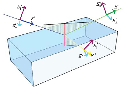
Figure 13: Resolution of electric fields.

The ratio of the amplitudes of the reflected and the transmitted electric fields is given by Fresnel reflection ($\Gamma$) and transmission (${T}$) coefficients. Fresnel coefficients depend on the polarization of the incident field. For a field polarized in the direction perpendicular to the plane of incidence, Fresnel coefficients are [4]

$${\Gamma}_{\bot}{=}\frac{{{E}}^{{r}}_{\bot}}{{{E}}^{{i}}_{\bot}}{=}\frac{{{n}}_{{2}}{\cos{\theta}^{{i}}\ }{-}{{n}}_{{1}}{\cos{\theta}^{{t}}\ }}{{{n}}_{{2}}{\cos{\theta}^{{i}}\ }{+}{{n}}_{{1}}{\cos{\theta}^{{t}}\ }}$$ (8)

$${{T}}_{\bot}{=}\frac{{{E}}^{{t}}_{\bot}}{{{E}}^{{i}}_{\bot}}{=}\frac{{2}{{n}}_{{2}}{\cos{\theta}^{{i}}\ }}{{{n}}_{{2}}{\cos{\theta}^{{i}}\ }{+}{{n}}_{{1}}{\cos{\theta}^{{t}}\ }}$$ (9)

While for a field polarized in the direction parallel to the plane of incidence, Fresnel coefficients are :

$${\Gamma}_{\parallel}{=}\frac{{{E}}^{{r}}_{\parallel}}{{{E}}^{{i}}_{\parallel}}{=}\frac{{-}{{n}}_{{1}}{\cos{\theta}^{{i}}\ }{+}{{n}}_{{1}}{\cos{\theta}^{{t}}\ }}{{{n}}_{{1}}{\cos{\theta}^{{i}}\ }{+}{{n}}_{{2}}{\cos{\theta}^{{t}}\ }}$$ (10)

$${{T}}_{\bot}{=}\frac{{{E}}^{{t}}_{\bot}}{{{E}}^{{i}}_{\bot}}{=}\frac{{2}{{n}}_{{2}}{\cos{\theta}^{{i}}\ }}{{{n}}_{{1}}{\cos{\theta}^{{i}}\ }{+}{{n}}_{{2}}{\cos{\theta}^{{t}}\ }}$$ (11)

Where

• $n_{1}$ is the absolute refractive index of the first medium.

• $n_{2}$ is the absolute refractive index of the second medium.

• $\theta^{i}$ is the angle of incidence.

• $\theta^{t}$ is the angle of transmission obtained from Snell’s Law 2.

The reflected field can be expressed in terms of the incident field and Fresnel reflection coefficients as

$$E^{r}=\left(E^{i}\cdot{\hat{e}}^{i}_{\parallel}\right){\Gamma}_{\parallel}{\hat{e}}^{r}_{\parallel}+\left(E^{i}\cdot{\hat{e}}^{i}_{\bot}\right){\Gamma}_{\bot}{\hat{e}}^{r}_{\bot}=E^{i}_{\parallel}{\Gamma}_{\parallel}{\hat{e}}^{r}_{\parallel}+E^{i}_{\bot}{\Gamma}_{\bot}{\hat{e}}^{r}_{\bot}$$ (12)

Similarly, the transmitted field can be expressed in terms of the incident field and Fresnel transmission coefficients as

$$E^{t}=\left(E^{i}\cdot{\hat{e}}^{i}_{\parallel}\right){{T}}_{\parallel}{\hat{e}}^{t}_{\parallel}+\left(E^{i}\cdot{\hat{e}}^{i}_{\bot}\right){{T}}_{\bot}{\hat{e}}^{t}_{\bot}=E^{i}_{\parallel}{{T}}_{\parallel}{\hat{e}}^{t}_{\parallel}+E^{i}_{\bot}{{T}}_{\bot}{\hat{e}}^{t}_{\bot}$$ (13)

A negative reflection coefficient means an increase in the phase shift by $180^{\circ}$.

By the summation of the two components using vector sum, the amplitude and the polarization of the resultant the reflected or the transmitted field is obtained.

The incident ray tube is spherical, ${\rho}^{i}_{1}={\rho}^{i}_{2}=\rho$, and all surfaces are assumed planar. The radii of curvature of the reflected and transmitted ray tubes then reduce to

$${\rho}^{r,t}_{1}={\rho}^{r,t}_{2}=\rho_{s}$$ (14)

A.3 Wedge Diffraction

A shadow region is the area that a GO ray can’t reach due to the presence of obstacles in its path. A shadow boundary is a boundary that defines the shadow region. 14 shows that there exist shadow regions for direct and reflected rays. GO is not sufficient to model these regions since it predicts Zero electric field in the shadow regions. Our model uses the Uniform Theory of Diffraction (UTD) to model wedge diffraction because of its ability to accurately predict the electric field in the shadow regions as well as its ability to give a non singular solution at the transition regions.

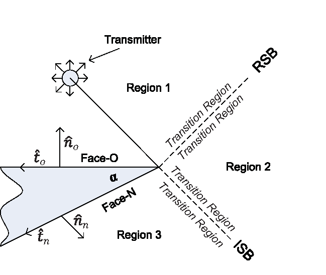
Figure 14: Shadow regions.

Figure 14 shows the geometry of a wedge. A wedge consists of two faces, O-face and N-face, and an edge. Each face has unit tangent and normal vectors. Tangents are directed away from the edge while normals are directed towards the outside of the wedge. The inner angle of the wedge is $\alpha$.

The plane of incidence is defined by ${\hat{s}}^{{}^{\prime}}$ and $\hat{e}$, while the plane of diffraction is defined by $\hat{s}$ and $\hat{e}$.

The incident electric field is resolved into two components parallel (${\widehat{\beta}}^{{}^{\prime}}_{0}$) and perpendicular (${\hat{\varphi}}^{{}^{\prime}}$) to the plane of incidence. The diffracted electric field is also resolved into two components parallel ($\widehat{\beta}$) and perpendicular ($\hat{\varphi}$) to the plane of diffraction.

A.3.1 Diffracted Electric Field

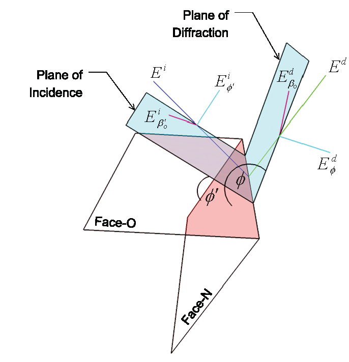
Figure 15: Resolution of electric fields.

Using figure 15, the incident electric field can be expressed as

$$E^{i}=E^{i}_{{\beta}^{{}^{\prime}}_{o}}{\widehat{\beta}}^{{}^{\prime}}_{0}+E^{i}_{\phi^{{}^{\prime}}}{\hat{\phi}}^{{}^{\prime}}$$ (15)

and the diffracted electric field can be expressed as

$$E^{d}=E^{d}_{{\beta}_{0}}{\widehat{\beta}}_{0}+E^{d}_{\phi}\hat{\phi}$$ (16)

The diffracted electric field at a distance $s$ on the path of the diffracted ray is given by

$$E^{d}=D.E^{i}.A\left(s\right)e^{-jks}$$ (17)

Where :

• D is the UTD diffraction coefficient.

  $$D=\left[\begin{array}[]{cc}-D_{s}&0\\ 0&-D_{h}\end{array}\right]$$ (18)

• A(s) is the spreading factor defined by:

  $$A\left(s\right)=\sqrt{\frac{\rho}{s\left(\rho+s\right)}}$$ (19)

• $\rho$ is the radius of curvature of the incident ray tube at the point of intersection with the edge.

A.3.2 UTD Diffraction Coefficients for PEC wedges

$$D_{s,h}\left(L^{i},L^{ro},L^{rn},\phi,\phi^{{}^{\prime}},{\beta}_{0},n\right)=D_{1}+D_{2}+R_{s,h}(D_{3}+D_{4})$$ (20)

Where $R_{s,h}$ are the reflection coefficients of the wedge at the edge. For a PEC surface $R_{s}=-1$ and $R_{h}=1$.

The components of the diffraction coefficients are given by

$$D_{1}=\frac{-e^{-j\frac{\pi}{4}}}{2n\sqrt{2\pi k}{\sin{\beta}_{0}\ }}{\cot\left[\frac{\pi+(\phi-\phi^{{}^{\prime}})}{2n}\right]F\left[kL^{i}a^{+}(\phi-\phi^{{}^{\prime}})\right]\ }$$ (21)

$$D_{2}=\frac{-e^{-j\frac{\pi}{4}}}{2n\sqrt{2\pi k}{\sin{\beta}_{0}\ }}{\cot\left[\frac{\pi-(\phi-\phi^{{}^{\prime}})}{2n}\right]F\left[kL^{i}a^{-}(\phi-\phi^{{}^{\prime}})\right]\ }$$ (22)

$$D_{3}=\frac{-e^{-j\frac{\pi}{4}}}{2n\sqrt{2\pi k}{\sin{\beta}_{0}\ }}{\cot\left[\frac{\pi+(\phi+\phi^{{}^{\prime}})}{2n}\right]F\left[kL^{rn}a^{+}(\phi+\phi^{{}^{\prime}})\right]\ }$$ (23)

$$D_{4}=\frac{-e^{-j\frac{\pi}{4}}}{2n\sqrt{2\pi k}{\sin{\beta}_{0}\ }}{\cot\left[\frac{\pi-(\phi+\phi^{{}^{\prime}})}{2n}\right]F\left[kL^{ro}a^{-}(\phi+\phi^{{}^{\prime}})\right]\ }$$ (24)

The functions a$\pm$ are defined as:

$$a^{\pm}\left({\beta}^{\pm}\right)=2{{\cos}^{{2}}\left(\frac{2n\pi N^{\pm}-{\beta}^{\pm}}{2}\right)\ }$$ (25)

The meaning and values of the parameters included can be obtained from [14].

A.3.3 UTD Diffraction Coefficients for non-PEC wedges

A number of heuristics were made to derive an expression for the diffraction coefficients for non-PEC surfaces. One of these heuristics uses Fresnel reflection and transmission coefficients as follows [22]

$$D_{s}\left(L^{i},L^{ro},L^{rn},\phi,\phi^{{}^{\prime}},{\beta}_{0},n\right)=D_{1}+D_{2}+{\Gamma}^{{n}}_{\parallel}D_{3}+{\Gamma}^{{o}}_{\parallel}D_{4}$$ (26)

$$D_{h}\left(L^{i},L^{ro},L^{rn},\phi,\phi^{{}^{\prime}},{\beta}_{0},n\right)=D_{1}+D_{2}+{\Gamma}^{{n}}_{\bot}D_{3}+{\Gamma}^{{o}}_{\bot}D_{4}$$ (27)

Where

• ${\Gamma}^{{o}}_{\parallel}$ and ${\Gamma}^{{n}}_{\parallel}$ are Fresnel’s reflection coefficients for parallel polarization of the o-Face and n-Face respectively.

• ${\Gamma}^{{o}}_{\bot}$ and ${\Gamma}^{{n}}_{\bot}$ are Fresnel’s reflection coefficients for perpendicular polarization of the o-Face and n-Face respectively.

Appendix B Human Modeling

In order to predict the human body-scattering effects in the indoor environment, a UTD-based propagation model is used. In the model, the human body is approximated with a perfect conducting circular cylinder[7] of radius 0.20 m, and height of 2 m. At microwave frequencies and higher, the human body constitutes a perfectly conducting and impassible reflector for electromagnetic waves [7].

B.1 Geometrical Configuration

An incident ray on a cylindrical surface may be either reflected or diffracted, according to the location of intersection between the ray and the cylindrical surface. A ray that falls tangential to the cylinder grazes the surface in the same plane of incidence. An extension of the incident ray beyond the point of grazing at the convex surface of the cylinder defines the Shadow Boundary (SB), which splits the space outside the surface into the lit and shadow regions [14].

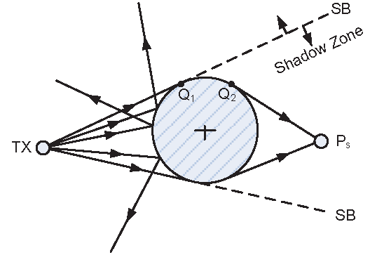
Figure 16: Geometrical configuration of the human shadowing problem.

Regions in the vicinity of the shadow boundary are called the transition regions. It is at the transition regions where the GO and GTD model fails as the incident field drops to zero, and the predicted field becomes infinite, and thus UTD was introduced [14]. Reflected rays from the cylinder falls in the lit region, while grazing rays detach from the surface into diffracted rays and fall in the shadow zone, which is the non-illuminated exterior region of the cylinder. A grazing ray path is determined by the shortest distance from the ray source to an observation point $P_{s}$, and creeping on the cylindrical surface [14].

B.2 Reflection Off a Cylindrical Surface

The UTD expression of the field reflected off a cylindrical surface from an incident electric field is given by [14]:

$$E^{r}\left(p\right)=E^{i}\left(Q_{r}\right)\cdot R_{s,h}\cdot A\left(s\right)\cdot e^{-jks^{r}}$$ (28)

Where:

• $E^{i}\left(Q_{r}\right)$ is the electric field incident to the cylinder at $Q_{r}$.

• $R_{s,h}$ are the soft and hard UTD reflection coefficients.

• $A\left(s\right)$ is the 3-D spreading factor of reflection.

• $e^{-jks^{r}}$ is the phase shift of the reflected field.

• $s^{r}$ is the distance between reflection point and observation point.

The soft and hard reflection coefficients are calculated from the following expression [14]:

$$R_{s,h}=-\sqrt{\frac{-4}{\xi}}\cdot e^{-j\pi/4}\cdot e^{-j{\xi}^{3}/12}\left[\frac{-F(X_{p})}{2\xi\sqrt{\pi}}+\left\{\begin{array}[]{c}p^{*}(\xi)\\ q^{*}(\xi)\end{array}\right\}\right]$$ (29)

Where:

• $p^{*}(\xi)$ and $q^{*}\left(\xi\right)$ are the soft and hard Fock scattering functions.

• $F(X_{p})$ is the UTD reflection transition function which ensures that fields surrounding the transition regions remains bounded.

• $X_{p}{(}\geq 0)$ is the transition function parameter, which is defined from [17]:

$$X_{p}=2kL_{p}{\cos}^{2}\left({\theta}^{i}\right)$$ (30)

Where $\xi(\leq 0)$ is the Fock parameter. It is defined from [17]:

$$\xi=-2m\left(Q_{r}\right){\cos}({\theta}^{i})$$ (31)

Where $m\left(Q_{r}\right)$ is the curvature parameter at the reflection point. It is calculated as [14]:

$$m\left(Q_{r}\right)={\left[\frac{ka_{t}(Q_{r})}{2}\right]}^{1/3}$$ (32)

Where $a_{t}(Q_{r})$ is the radius of curvature of the surface in the plane of incidence at $Q_{r}$. Computation-friendly expressions for the transition and the scattering functions can be found in [14], and [5].

$L_{p}$ is the 3-D distance parameter, which is calculated from [17]:

$$L_{p}=\frac{{\rho}^{i}_{1}{\rho}^{i}_{2}}{\left({\rho}^{i}_{1}+s^{r}\right)\left({\rho}^{i}_{2}+s^{r}\right)}\cdot\frac{s^{r}\left({\rho}^{r}_{2}+s^{r}\right)}{{\rho}^{r}_{2}}$$ (33)

Where:

• ${\rho}^{i}_{1}$ (${\rho}^{i}_{2}$) is the radius of curvature of the incident wave in (transverse to) the plane of incidence.

• ${\rho}^{r}_{2}$ is the radius of curvature of the reflected wave transverse to the plane of reflection.

In our implementation, waves are assumed to be spherical. In that case, ${\rho}^{i}_{1}={\rho}^{i}_{2}=s^{i}$ where $s^{i}$ is the total unfolded distance from the transmitter to the point of reflection. The reflected wavefront radii of curvature are calculated from [14]:

$$\frac{1}{{\rho}^{r}_{1,2}}=\frac{1}{s^{i}}+\frac{1}{f_{1,2}}$$ (34)

Where:

$$f_{1,2}=\frac{1}{\cos(\theta^{i})}\left[\frac{\sin^{2}(\theta_{2})}{a_{1}}+\frac{\sin^{2}(\theta_{1})}{a_{2}}\right]\\ \pm{\left[\frac{1}{\cos^{2}(\theta^{i})}\left(\frac{\sin^{2}(\theta_{2})}{a_{1}}+\frac{\sin^{2}(\theta_{1})}{a_{2}}\right)-\frac{4}{a_{1}a_{2}}\right]}^{1/2}$$ (35)

The terms $a_{1}$and $a_{2}$ are the principal radii of curvature of the surface at the incidence point. They measure how the surface bends by different amounts in different directions at a given point. In the case of a circular cylinder, $a_{1}=radius$ and $a_{2}=infinity$, hence the previous expression reduces to:

$$f_{1,2}=\frac{1}{{\cos}({\theta}^{i})}\left[\frac{{{\sin}}^{{2}}({\theta}_{2})}{a_{1}}\right]\pm{\left[\frac{1}{{{\cos}}^{{2}}({\theta}^{i})}\left(\frac{{{\sin}}^{{2}}({\theta}_{2})}{a_{1}}\right)\right]}^{1/2}$$ (36)

The quantities ${{\sin}}^{{2}}({\theta}_{1})$ and ${{\sin}}^{{2}}({\theta}_{2})$ are calculated from [14]:

$${{\sin}^{{2}}\left({\theta}_{1}\right)\ }={{\cos}^{{2}}\left(\alpha\right)\ }+{{\sin}}^{{2}}(\alpha){\ }{{\cos}}^{{2}}(\theta^{i})$$ (37)

$${{\sin}^{{2}}\left({\theta}_{2}\right)\ }={{\sin}^{{2}}\left(\alpha\right)\ }+{{\cos}}^{{2}}(\alpha){\ }{{\cos}}^{{2}}(\theta^{i})$$ (38)

Where $\alpha$ is the angle between the principal plane of the surface at the point of incidence and the plane of incidence as shown in Figure 17.

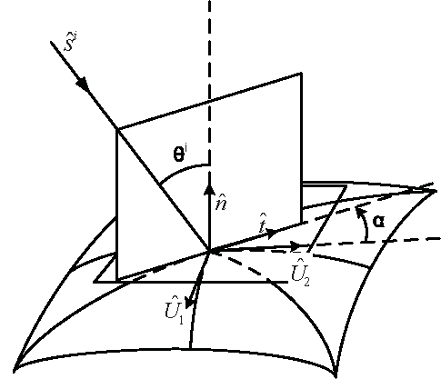
Figure 17: Principal directions at the point of incidence.

The value of $\alpha$ is calculated from [17]:

$$t_{1}=-{\hat{s}}^{i}\cdot{\hat{U}}_{1}$$ (39)

$$t_{2}=-{\hat{s}}^{i}\cdot{\hat{U}}_{2}$$ (40)

$$\alpha=\left|{\tan^{-1}\frac{t_{1}}{t_{2}}\ }\right|$$ (41)

Where ${\hat{U}}_{1}$ and ${\hat{U}}_{2}$ are the principal directions of the surface at the point of incidence. In the case of a cylindrical surface, ${\hat{U}}_{2}$ is parallel to the cylinder generator, and ${\hat{U}}_{1}$ is perpendicular to ${\hat{U}}_{2}$.

Finally, the reflected spherical wave front radii are calculated as:

$${\rho}^{r}_{1,2}=\frac{\rho^{r}_{1}+\rho^{r}_{2}}{2}$$ (42)

When an incident field reflects from a cylindrical surface, the reflected field amplitude varies from that of the incident field. The 3-D spreading factor governs the amplitude variation of the reflected field in 3D. It is calculated from [17]:

$$A\left(s\right)=\sqrt{\frac{{\rho}^{r}_{1}{\rho}^{r}_{2}}{\left({\rho}^{r}_{1}+s^{r}\right)\left({\rho}^{r}_{2}+s^{r}\right)}}$$ (43)

B.3 Diffraction Off a Cylindrical Surface

An incident tangential ray at $Q_{1}$ creeps the cylinder surface and detaches at $Q_{2}$. The location of $Q_{2}$ depends on the location of the observation point so that the total distance from the point of incidence to the observation point, including the creeping distance, is minimal.

The field diffracted from a cylindrical surface is given by [17]:

$$E^{d}\left(p\right)=E^{i}\left(Q_{1}\right)\cdot T_{s,h}\cdot EC\cdot A\left(s\right)\cdot e^{-jks^{r}}$$ (44)

Where:

• $E^{i}\left(Q_{1}\right)$ is the incident field on the cylinder at $Q_{1}$.

• $T_{s,h}$ are the soft and hard UTD diffraction coefficient.

• $A\left(s\right)=\sqrt{\frac{\rho^{r}_{2}}{s^{r}\left(\rho^{r}_{2}+s^{r}\right)}}$ is the 3-D spreading factor of diffraction.

• $EC=\sqrt{\frac{\rho^{i}_{2}}{\rho^{i}_{2}+t}}$ is the conservation of energy term in the case of spherical waves, where $t$ is the creep distance along the surface from $Q_{1}$ to $Q_{2}$.

The soft and hard UTD diffraction coefficients are given by [17]:

$$T_{s,h}=-\sqrt{m(Q_{1})m(Q_{2})}\cdot\sqrt{\frac{2}{k}}\cdot e^{-j\pi/4}\cdot e^{-jk}\\ \cdot\left[\frac{-F(X_{d})}{2\xi\sqrt{\pi}}+\left\{\begin{array}[]{c}p^{*}(\xi)\\ q^{*}(\xi)\end{array}\right\}\right]$$ (45)

Where:

• $F(X_{d})$ is the diffraction transition function.

• $X_{d}=\frac{kL_{d}\xi^{2}}{2m\left(Q_{1}\right)m(Q_{2})}$ is the transition function argument.

• $L_{d}$ is the 3-D distance parameter.

• $\xi=\int_{t}{\frac{m(Q_{t})}{a_{t}}}$ is the Fock parameter.

Transition and Fock functions are computed as described in the previous section.

The two radii of curvature of the diffracted wave at the observation point are calculated from [17]:

$$\rho^{r}_{1}=\rho^{i}_{b}+s^{r}+t\rho^{r}_{2}=s^{r}$$ (46)

Where:

• $t$ is the creeping distance.

• $s^{r}$ is the distance between the observation point and the detachment point $Q_{2}$.

• $\rho^{i}_{b}$ is the radius of curvature of the incident wave in the plane transverse to the incident plane, which is calculated from [17]:

$$\frac{1}{\rho^{i}_{b}}=\frac{\sin^{2}(\alpha)}{\rho^{i}_{1}}+\frac{\cos^{2}(\alpha)}{\rho^{i}_{2}}$$ (47)

As we assume spherical waves, that is $\rho^{i}_{1}=\rho^{i}_{2}=s^{i}$, the previous equation reduces to:

$$\rho^{i}_{b}=\rho^{i}_{1}=\rho^{i}_{2}$$ (48)

The final radii of curvature of the diffracted ray are then calculated as the average of its two radii of curvature.

References

- [1] H. A., M. K., and G. M. Mesh Edge Detection. Technical Report 351, Swiss Federal Institute of Technology, 2000.
- [2] G. Athanasiadou and A. Nix. A Novel 3-d Indoor Ray-Tracing Propagation Model : the Path Generator and Evaluation of Narrow-band and Wide-band Predictions. In IEEE Transactions on Vehicular Technology, volume 49(4), pages 1152–1168. IEEE, July 2000.
- [3] P. Bahl and V. N. Padmanabhan. RADAR: An In-Building RF-based User Location and Tracking System. In IEEE INFOCOM 2000, volume 2, pages 775–784. IEEE, March 2000.
- [4] M. Born and E. Wolf. Principles of Optics: Electromagnetic Theory of Propagation, Interference and Diffraction of Light (7th Edition). Cambridge University Press, 7th edition, 1999.
- [5] W. Burnside, R. Marhefka, and N. Wang. Computer Programs, Subroutines and Functions for the Short Course on the Modern Geometrical Theory of Diffraction. In Appendices for the Short Course on Applications of the Modern Geometrical Theory of Difraction. Ohio State University, 1984.
- [6] D. G., P. N., and R. T. S. An Advanced 3d Ray Launching Method for Wireless Propagation Prediction. In IEEE Vehicular Technology Conference 47th, 1997.
- [7] M. Ghaddar, L. Talbi, T. Denid, and A. Charbonneau. Modeling Human Body Effects for Indoor Radio Channel using UTD. In Electrical and Computer Engineering, 2004. Canadian Conference on. IEEE, 2004.
- [8] M. Hassan-Ali and K. Pahlavan. A new statistical model for site-specific indoor radio propagation prediction based on geometric optics and geometric probability. In Wireless Communications, IEEE Transactions on, volume 1, pages 112–124, 1 2002.
- [9] A. Hills, J. Schlegel, and B. Jenkins. Estimating signal strengths in the design of an indoor wireless network. In Wireless Communications, IEEE Transactions on, volume 3, pages 17–19, 1 2004.
- [10] Y. Ji and S. Biaz. ARIADNE: A Dynamic Indoor Signal Map Construction and Localization System. In in MobiSys 2006: Proceedings of the 4th international conference on Mobile systems, applications and services, pages 151–164. ACM Press, 2006.
- [11] J. B. KELLER. Geometrical theory of diffraction. J. Opt. Soc. Am., 52(2):116–130, 1962.
- [12] M. Lawton and J. McGeehan. The Application of a Deterministic Ray Launching Algorithm for the Prediction of Radio Channel Characteristics in Small-Cell Environments. In IEEE Transactions on Vehicular Technology, volume 43(4), pages 955–968. IEEE, November 1994.
- [13] Y. M., M. M., and A. A. Device-free Passive Localization. Technical Report CSH860, Department of Computer Science, University of Maryland, 2007.
- [14] D. A. Mcnamara, C. W. I. Pistorius, and J. A. G. Malherbe. Introduction to the Uniform Geometrical Theory of Diffraction. Artech House Publishers, 1990.
- [15] Microsoft. NDISProt. Online.
- [16] Microsoft. Overview of NDIS Network Interfaces. Online.
- [17] P. P.H, B. W.D, and M. R.J. A Uniform GTD Analysis of the Diffraction of Electromagnetic waves by a Smooth Convex Surface. In IEEE Trans. Antennas Propagat, volume AP-28, pages 631–642. IEEE, 1980.
- [18] M. Powell. jMonkeyEngine. Online.
- [19] T. Roos, P. Myllymaki, H. Tirri, P. Misikangas, and J. Sievanen. A Probabilistic Approach to WLAN User Location Estimation. In International Journal of Wireless Information Networks, volume 9(3), July 2002.
- [20] S. Seidel and T. Rappaport. Site-Specific Propagation Prediction for Wireless In-Building Personal Communication System Design. In IEEE Trans. Vehicular Technology, volume 43, pages 879–891, 1994.
- [21] J. M. V. Verth and L. M. Bishop. ESSENTIAL MATHEMATICS FOR GAMES AND INTERACTIVE APPLICATIONS. Morgan Kaufmann, second edition, 2004.
- [22] Y. Wang. Site-Specific Modeling of Indoor Radio Wave Propagation. PhD thesis, Waterloo, Ontario, Canada, 2000.
- [23] C. Yang, B. Wu, and C. Ko. A Ray-Tracing Method for Modeling Indoor Wave Propagation and Penetration. In IEEE Transactions on Antennas and Propagation, volume 46, pages 907–919. IEEE, June 1998.
- [24] M. Youssef, M. Mah, and A. Agrawala. Challenges: Device-free Passive Localization for Wireless Environments. In MobiCom ’07: Proceedings of the 13th annual ACM international conference on Mobile computing and networking, pages 222–229. ACM, 2007.
- [25] M. A. Youssef and A. Agrawala. The Horus WLAN Location Determination System. In Communication Networks and Distributed Systems Modeling and Simulation Conference, pages 205–218, 2005.
- [26] M. A. Youssef, A. Agrawala, and Udaya. WLAN location determination via clustering and probability distributions. In Pervasive Computing and Communications, 2003. (PerCom 2003). Proceedings of the First IEEE International Conference on, pages 143–150, 2003.