New parametrization for the nuclear covariant energy density functional with point-coupling interaction

Abstract

A new parametrization PC-PK1 for the nuclear covariant energy density functional with nonlinear point-coupling interaction is proposed by fitting to observables of 60 selected spherical nuclei, including the binding energies, charge radii and empirical pairing gaps. The success of PC-PK1 is illustrated in the description for infinite nuclear matter and finite nuclei including the ground-state and low-lying excited states. Particularly, PC-PK1 provides good description for isospin dependence of binding energy along either the isotopic or the isotonic chains, which makes it reliable for application in exotic nuclei. The predictive power of PC-PK1 is also illustrated for the nuclear low-lying excitation states in a five-dimensional collective Hamiltonian in which the parameters are determined by constrained calculations for triaxial shapes.

I Introduction

In the past years, the unstable nuclear beams have extended our knowledge of nuclear physics from the stable nuclei to the unstable nuclei far from the stability line — so-called “exotic nuclei”. Extensive research in this area shows a lot of entirely unexpected features and novel aspects of nuclear structure such as the halo phenomenon Tanihata et al. (1985); Meng and Ring (1996, 1998), the disappearance of traditional magic numbers and the occurrence of new ones Ozawa et al. (2000). The exotic nuclei play important roles in nuclear astrophysics, since their properties are crucial to stellar nucleosynthesis. To understand the physics in exotic nuclei, it becomes very important to find a reliable theory and improve the reliability for predicting the properties of more exotic nuclei close to proton and neutron drip lines.

Nuclear energy density functional (EDF) theory Bender et al. (2003) has played an important role in a self-consistent description of nuclei. With a few parameters, EDF theory is able to give a satisfactory description for the ground state properties of spherical and deformed nuclei all over the nuclide chart. Detailed discussion on the EDF theory can be seen in Ref. Fayans et al. (2000) for nonrelativistic representations and in Refs. Vretenar et al. (2005); Meng et al. (2006) for relativistic ones.

There exist a number of attractive features in the covariant EDF theory, especially in its practical applications of self-consistent relativistic mean-field (RMF) framework Vretenar et al. (2005); Meng et al. (2006). The most obvious one is the natural inclusion of the nucleon spin degree of freedom and the resulting nuclear spin-orbit potential that emerges automatically with the empirical strength in a covariant way. The relativistic effects are responsible for the empirical existence of approximate pseudospin symmetry in the nuclear single-particle spectra Ginocchio (2005). Moreover, a covariant treatment of nuclear matter provides a distinction between scalar and four-vector nucleon self energies, leading to a natural saturation mechanism.

The most widely used RMF framework is based on the finite-range meson-exchange representation (RMF-FR), in which the nucleus is described as a system of Dirac nucleons which interact with each other via the exchange of mesons. The isoscalar-scalar $\sigma$ meson, the isoscalar-vector $\omega$ meson, and the isovector-vector $\rho$ meson build the minimal set of meson fields that, together with the electromagnetic field, is necessary for a description of bulk and single-particle nuclear properties. Moreover, a quantitative treatment of nuclear matter and finite nuclei needs a medium dependence of effective mean-field interactions, which can be introduced by including nonlinear meson self-interaction terms in the Lagrangian or by assuming explicit density dependence for the meson-nucleon couplings. Of course, at the energy characteristic for nuclear binding and low-lying excited states, the heavy-meson exchange ($\sigma$, $\omega$, $\rho$) is just a convenient representation of the effective nuclear interaction.

Since the exchange of heavy mesons is associated with short-distance dynamics that cannot be resolved at low energies, as an alternative, the relativistic point-coupling (RMF-PC) model Nikolaus et al. (1992); Bürvenich et al. (2002) is proposed by using the zero-range point-coupling interaction instead of the meson exchange, i.e., in each channel (scalar-isoscalar, vector-isoscalar, scalar-isovector, and vector-isovector) meson exchange is replaced by the corresponding local four-point (contact) interaction between nucleons. Analogously, in the case of contact interactions, the medium effects can be taken into account by including higher-order (nonlinear coupling) interaction terms or by assuming a density dependence of strength parameters for the coupling interactions.

In recent years, the RMF-PC model has attracted more and more attentions due to the following advantages. Firstly, it avoids the possible physical constrains introduced by explicit usage of the Klein-Gordon equation to describe mean meson fields, especially the fictitious $\sigma$ meson. Secondly, it is possible to study the role of naturalness Friar et al. (1996); Manohar and Georgi (1984) in effective theories for nuclear structure related problems. Thirdly, it provides more opportunities to investigate its relationship to the nonrelativistic approaches Sulaksono et al. (2003). Finally, it is relatively easy to study the effects beyond mean-field for the nuclear low-lying collective excited states.

In practical application of the RMF-PC model, the most widely used nonlinear coupling parameterizations include PC-LA Nikolaus et al. (1992) and PC-F1 Bürvenich et al. (2002). PC-LA is determined by the ground-state observables of ${}^{16}\rm O$, ${}^{88}\rm Sr$, and ${}^{208}\rm Pb$. Due to the explicit omission of the pairing interaction, the pairing effects are not included in the fitting procedure. Moreover, the test for naturalness in Ref. Friar et al. (1996) shows that only six of the nine coupling constants are natural. As an improvement, PC-F1 is optimized to observables of 17 spherical nuclei including open-shell nuclei, and the pairing correlation is considered through a standard BCS approach in the fitting procedure. Furthermore, all the coupling constants of PC-F1 are turned out to be natural Bürvenich et al. (2002). However, the isospin dependence of binding energy given by PC-F1 along either the isotopic or the isotonic chains deviates from the data remarkably.

Recently, a density-dependent parametrization DD-PC1 is proposed from the equation of state (EOS) of nuclear matter and the masses of 64 axially deformed nuclei in the mass regions $A\simeq 150-180$ and $A\simeq 230-250$ Nikšić et al. (2008). Although it reproduces the binding energies, deformations, and charge radii of deformed nuclei quite well, the differences between the predicted binding energies and the corresponding data are somewhat large for spherical nuclei.

Therefore, it is necessary to have a new parametrization for the nuclear covariant energy density functional with point-coupling interaction to describe both the nuclear matter and finite nuclei properties. In this work, a new parametrization PC-PK1 with nonlinear coupling interactions is proposed. In Sec. II, the theoretical framework for the relativistic point-coupling model is briefly outlined. The numerical details are given in Sec. III. In Sec. IV-VII, a series of illustrative descriptions for the nuclear matter, spherical nuclei, deformed nuclei as well as the nuclear excited properties are presented. Finally, a summary is given in Sec. VIII.

II Theoretical framework

The basic building blocks of RMF theory with point-coupling vertices are

$$(\bar{\psi}{\cal O}\Gamma\psi),~{}~{}~{}~{}~{}{\cal O}\in\{1,\vec{\tau}\},~{}~{}~{}~{}~{}\Gamma\in\{1,\gamma_{\mu},\gamma_{5},\gamma_{5}\gamma_{\mu},\sigma_{\mu\nu}\},$$ (1)

where $\psi$ is Dirac spinor field of nucleon, $\vec{\tau}$ is the isospin Pauli matrix, and $\Gamma$ generally denotes the $4\times 4$ Dirac matrices. There are ten such building blocks characterized by their transformation characteristics in isospin and Minkowski space. In this paper, vectors in the isospin space are denoted by arrows and the space vectors by bold type. Greek indices $\mu$ and $\nu$ run over the Minkowski indices $0$, $1$, $2$, and $3$.

A general effective Lagrangian can be written as a power series in $\bar{\psi}{\cal O}\Gamma\psi$ and their derivatives. We start with the following Lagrangian density of the point-coupling model

$${\cal L}={\cal L}^{\rm free}+{\cal L}^{\rm 4f}+{\cal L}^{\rm hot}+{\cal L}^{\rm der}+{\cal L}^{\rm em},$$ (2)

which is divided as the Lagrangian density for free nucleons ${\cal L}^{\rm free}$,

$${\cal L}^{\rm free}=\bar{\psi}(i\gamma_{\mu}\partial^{\mu}-m)\psi,$$ (3)

the four-fermion point-coupling terms ${\cal L}^{\rm 4f}$,

$${\cal L}^{\rm 4f} = -\frac{1}{2}\alpha_{S}(\bar{\psi}\psi)(\bar{\psi}\psi)-\frac{1}{2}\alpha_{V}(\bar{\psi}\gamma_{\mu}\psi)(\bar{\psi}\gamma^{\mu}\psi)$$ (4)

$$-\frac{1}{2}\alpha_{TS}(\bar{\psi}\vec{\tau}\psi)(\bar{\psi}\vec{\tau}\psi)-\frac{1}{2}\alpha_{TV}(\bar{\psi}\vec{\tau}\gamma_{\mu}\psi)(\bar{\psi}\vec{\tau}\gamma^{\mu}\psi),$$

the higher order terms ${\cal L}^{\rm hot}$ which are responsible for the effects of medium dependence,

$${\cal L}^{\rm hot}=-\frac{1}{3}\beta_{S}(\bar{\psi}\psi)^{3}-\frac{1}{4}\gamma_{S}(\bar{\psi}\psi)^{4}-\frac{1}{4}\gamma_{V}[(\bar{\psi}\gamma_{\mu}\psi)(\bar{\psi}\gamma^{\mu}\psi)]^{2},$$ (5)

the gradient terms ${\cal L}^{\rm der}$ which are included to simulate the effects of finite-range,

$${\cal L}^{\rm der} = -\frac{1}{2}\delta_{S}\partial_{\nu}(\bar{\psi}\psi)\partial^{\nu}(\bar{\psi}\psi)-\frac{1}{2}\delta_{V}\partial_{\nu}(\bar{\psi}\gamma_{\mu}\psi)\partial^{\nu}(\bar{\psi}\gamma^{\mu}\psi)$$ (6)

$$-\frac{1}{2}\delta_{TS}\partial_{\nu}(\bar{\psi}\vec{\tau}\psi)\partial^{\nu}(\bar{\psi}\vec{\tau}\psi)-\frac{1}{2}\delta_{TV}\partial_{\nu}(\bar{\psi}\vec{\tau}\gamma_{\mu}\psi)\partial^{\nu}(\bar{\psi}\vec{\tau}\gamma_{\mu}\psi),$$

and the electromagnetic interaction terms ${\cal L}^{\rm em}$,

$${\cal L}^{\rm em}=-\frac{1}{4}F^{\mu\nu}F_{\mu\nu}-e\frac{1-\tau_{3}}{2}\bar{\psi}\gamma^{\mu}\psi A_{\mu}.$$ (7)

For the Lagrangian density in Eq. (2), $m$ is the nucleon mass and $e$ is the charge unit for protons. $A_{\mu}$ and $F_{\mu\nu}$ are respectively the four-vector potential and field strength tensor of the electromagnetic field. There are totally 11 coupling constants, $\alpha_{S}$, $\alpha_{V}$, $\alpha_{TS}$, $\alpha_{TV}$, $\beta_{S}$, $\gamma_{S}$, $\gamma_{V}$, $\delta_{S}$, $\delta_{V}$, $\delta_{TS}$, and $\delta_{TV}$, in which $\alpha$ refers to the four-fermion term, $\beta$ and $\gamma$ respectively the third- and fourth-order terms, and $\delta$ the derivative couplings. The subscripts $S$, $V$, and $T$ respectively indicate the symmetries of the couplings, i.e., $S$ stands for scalar, $V$ for vector, and $T$ for isovector.

From former experience Bürvenich et al. (2002), we neglect the isovector-scalar channel in Eq. (2) since a fit including the isovector-scalar interaction does not improve the description of nuclear ground-state properties. Consequently, there are nine free parameters in the present RMF-PC model, which are comparable with those in the RMF-FR model. Furthermore, the pseudoscalar $\gamma_{5}$ and pseudovector $\gamma_{5}\gamma_{\mu}$ channels are also neglected in Eq. (2) since they do not contribute at the Hartree level due to parity conservation in nuclei.

Similar to the RMF-FR case, the mean-field approximation leads to the replacement of the operators $\bar{\psi}(\hat{{\cal O}}\Gamma)_{i}\psi$ in Eq. (2) by their expectation values which become bilinear forms of the nucleon Dirac spinor $\psi_{k}$,

$$\bar{\psi}(\hat{{\cal O}}\Gamma)_{i}\psi\rightarrow\langle\Phi|\bar{\psi}(\hat{{\cal O}}\Gamma)_{i}\psi|\Phi\rangle=\sum\limits_{k}v_{k}^{2}\bar{\psi}_{k}(\hat{{\cal O}}\Gamma)_{i}\psi_{k},$$ (8)

where $i$ indicates $S$, $V$, and $TV$. The sum $\sum$ runs over only positive energy states with the occupation probabilities $v_{k}^{2}$, i.e., the “no-sea” approximation. Based on these approximations, one finds the energy density functional for a nuclear system

$$E_{\rm DF}[{\bm{\tau}},\rho_{S},j^{\mu}_{i},A_{\mu}]=\int d^{3}r~{}{\mathcal{E}(\bm{r}}),$$ (9)

with the energy density

$$\mathcal{E}(\bm{r})=\mathcal{E}^{\rm kin}(\bm{r})+\mathcal{E}^{\rm int}(\bm{r})+\mathcal{E}^{\rm em}(\bm{r}),$$ (10)

which is composed of a kinetic part

$$\mathcal{E}^{\rm kin}(\bm{r})=\sum_{k}\,v_{k}^{2}~{}{\psi^{\dagger}_{k}(\bm{r})\left(\bm{\alpha}\cdot\bm{p}+\beta m\right)\psi_{k}(\bm{r})},$$ (11)

an interaction part

$$\mathcal{E}^{\rm int}(\bm{r}) = \frac{\alpha_{S}}{2}\rho_{S}^{2}+\frac{\beta_{S}}{3}\rho_{S}^{3}+\frac{\gamma_{S}}{4}\rho_{S}^{4}+\frac{\delta_{S}}{2}\rho_{S}\triangle\rho_{S}$$

$$+\frac{\alpha_{V}}{2}j_{\mu}j^{\mu}+\frac{\gamma_{V}}{4}(j_{\mu}j^{\mu})^{2}+\frac{\delta_{V}}{2}j_{\mu}\triangle j^{\mu}$$

$$+\frac{\alpha_{TV}}{2}\vec{j}^{\mu}_{TV}\cdot(\vec{j}_{TV})_{\mu}+\frac{\delta_{TV}}{2}\vec{j}^{\mu}_{TV}\cdot\triangle(\vec{j}_{TV})_{\mu},$$

with the local densities and currents

$$\rho_{S}(\bm{r}) = \sum_{k}v^{2}_{k}\bar{\psi}_{k}(\bm{r})\psi_{k}(\bm{r}),$$ (13a)

$$j^{\mu}_{V}(\bm{r}) = \sum_{k}v^{2}_{k}\bar{\psi}_{k}(\bm{r})\gamma^{\mu}\psi_{k}(\bm{r}),$$ (13b)

$$\vec{j}^{\mu}_{TV}(\bm{r}) = \sum_{k}v^{2}_{k}\bar{\psi}_{k}(\bm{r})\vec{\tau}\gamma^{\mu}\psi_{k}(\bm{r}),$$ (13c)

and an electromagnetic part

$$\mathcal{E}^{\rm em}(\bm{r})=\frac{1}{4}F_{\mu\nu}F^{\mu\nu}-F^{0\mu}\partial_{0}A_{\mu}+eA_{\mu}j^{\mu}_{p}.$$ (14)

Minimizing the energy density functional Eq. (9) with respect to $\bar{\psi}_{k}$, one obtains the Dirac equation for the single nucleons

$$[\gamma_{\mu}(i\partial^{\mu}-V^{\mu})-(m+S)]\psi_{k}=0.$$ (15)

The single-particle effective Hamiltonian contains local scalar $S(\bm{r})$ and vector $V^{\mu}(\bm{r})$ potentials,

$$S(\bm{r})=\Sigma_{S},\quad V^{\mu}(\bm{r})=\Sigma^{\mu}+\vec{\tau}\cdot\vec{\Sigma}^{\mu}_{TV},$$ (16)

where the nucleon scalar-isoscalar $\Sigma_{S}$, vector-isoscalar $\Sigma^{\mu}$, and vector-isovector $\vec{\Sigma}^{\mu}_{TV}$ self-energies are given in terms of the various densities,

$$\Sigma_{S} = \alpha_{S}\rho_{S}+\beta_{S}\rho^{2}_{S}+\gamma_{S}\rho^{3}_{S}+\delta_{S}\triangle\rho_{S},$$ (17a)

$$\Sigma^{\mu} = \alpha_{V}j^{\mu}_{V}+\gamma_{V}(j^{\mu}_{V})^{3}+\delta_{V}\triangle j^{\mu}_{V}+eA^{\mu},$$ (17b)

$$\vec{\Sigma}^{\mu}_{TV} = \alpha_{TV}\vec{j}^{\mu}_{TV}+\delta_{TV}\triangle\vec{j}^{\mu}_{TV}.$$ (17c)

For a system with time reversal invariance, the space-like components of the currents $\bm{j}_{i}$ in Eq. (13) and the vector potential $\bm{V}(\bm{r})$ in Eq. (16) vanish. Furthermore, one can assume that the nucleon single-particle states do not mix isospin, i.e., the single-particle states are eigenstates of $\tau_{3}$. Therefore only the third component of isovector potentials $\vec{\Sigma}^{\mu}_{TV}$ survives. The Coulomb field $A_{0}$ is determined by Poisson’s equation.

In addition to the self-consistent mean-field potentials, for open-shell nuclei, pairing correlations are taken into account by the BCS method with a smooth cutoff factor $f_{k}$ to simulate the effects of finite-range Krieger et al. (1990); Bender et al. (2000a), i.e., we have to add to the functional Eq. (9) a pairing energy term of the form depending on the pairing tensor $\kappa$,

$$E_{\rm pair}[\kappa,\kappa^{*}]=\sum_{kk^{\prime}>0}f_{k}f_{k^{\prime}}\langle k{\bar{k}}|V^{pp}|k^{\prime}{\bar{k}}^{\prime}\rangle\kappa^{\ast}_{k}\kappa_{k^{\prime}},$$ (18)

with the smooth cut-off weight factor

$$f_{k}=\frac{1}{1+\exp[(\epsilon_{k}-\epsilon_{F}-\Delta E_{\tau})/\mu_{\tau}]},$$ (19)

where $\epsilon_{k}$ is the eigenvalue of the self-consistent single-particle field, and $\epsilon_{F}$ is the chemical potential determined by the particle number, $\langle\Phi|\hat{N}_{\tau}|\Phi\rangle=N_{\tau}$, with $N_{\tau}$ the particle number of neutron or proton. The cut-off parameters $\Delta E_{\tau}$ and $\mu_{\tau}=\Delta E_{\tau}/10$ are chosen in such a way that $2\displaystyle\sum_{k>0}f_{k}=N_{\tau}+1.65N^{2/3}_{\tau}$ Bender et al. (2000a).

In the following calculations, a density-independent $\delta$-force in the pairing channel is adopted. Thus, the pairing energy is given by

$$E_{\rm pair}[\kappa,\kappa^{*}]=-\sum_{\tau=n,p}\dfrac{V_{\tau}}{4}\int d^{3}r\kappa^{\ast}_{\tau}(\bm{r})\kappa_{\tau}(\bm{r}),$$ (20)

where $V_{\tau}$ is the constant pairing strength and the pairing tensor $\kappa(\bm{r})$ reads

$$\kappa(\bm{r})=-2\sum_{k>0}f_{k}u_{k}v_{k}|\psi_{k}(\bm{r})|^{2}.$$ (21)

The pairing strength parameters $V_{\tau}$ can be adjusted by fitting the average single-particle pairing gap

$$\langle\Delta\rangle\equiv\frac{\sum_{k}f_{k}u_{k}v_{k}\Delta_{k}}{\sum_{k}f_{k}u_{k}v_{k}}$$ (22)

to the data obtained with a five-point formula.

As the translational symmetry is broken in the mean-field approximation, proper treatment of center-of-mass (c.m.) motion is very important and here the c.m. correction energy is calculated by microscopic c.m. correction

$$E^{\rm mic}_{\rm c.m.}=-\frac{1}{2mA}\langle\hat{\bm{P}}^{2}_{\rm c.m.}\rangle,$$ (23)

with $A$ mass number and $\hat{\bm{P}}_{\rm c.m.}=\sum_{i}^{A}\hat{\bm{p}}_{i}$ the total momentum in the c.m. frame. It has been shown that the microscopic c.m. correction provides more reasonable and reliable results than phenomenological ones Bender et al. (2000b); Long et al. (2004); Zhao et al. (2009).

Therefore, the total energy for the nuclear system becomes

$$E_{\rm tot}=E_{\rm DF}[\bm{\tau},\rho_{S},j^{\mu}_{i},A_{\mu}]+E_{\rm pair}[\kappa,\kappa^{*}]+E^{\rm mic}_{\rm c.m.}.$$ (24)

III Numerical details

In this work, a series of calculations have been performed for both the spherical and deformed nuclei. The Dirac equation for nucleons is solved in a three-dimensional harmonic oscillator basis Gambhir et al. (1990). For spherical calculations, by increasing the fermionic shells from $N_{f}=20$ to $N_{f}=22$, the binding energy, charge radius, and neutron skin thickness in ${}^{208}\rm Pb$ change by 0.003%, 0.007%, and 0.1% respectively. For ${}^{240}\rm U$, the binding energy changes by 0.001% from the axially deformed calculation with $N_{f}=16$ to $N_{f}=18$. Therefore, a basis of 20 major oscillator shells is used in the spherical calculations and 16 shells in the axially deformed cases. The triaxial calculations are performed with $N_{f}=12$, which, for Nd isotopes, provides an accuracy of 0.04% for binding energies in comparison with the calculations with $N_{f}=14$. To achieve an accuracy of $\sim 100$ keV in the description of both the fission barrier and the energy of the isomer state in ${}^{240}\rm Pu$, a basis of 20 oscillator shells has been adopted in both the axial and triaxial calculations.

In order to determine the parameters of Lagrangian density in Eq. (2) and the pairing strength in Eq. (20), a multiparameter fitting to both the binding energies and charge radii for selected spherical nuclei is performed with the Levenberg-Marquardt method Press et al. (1992). As usual, the masses of neutron and proton are fixed as 939 MeV. The corresponding data Audi et al. (2003); De Vries et al. (1987); Nadjakov et al. (1994) for selected spherical nuclei used in the fitting procedure are listed in Table LABEL:Tabel:mass and 3. The empirical neutron pairing gaps for ${}^{122}\rm Sn$, ${}^{124}\rm Sn$, and ${}^{200}\rm Pb$ as well as the proton ones for ${}^{92}\rm Mo$, ${}^{136}\rm Xe$, and ${}^{144}\rm Sm$ obtained with five-point formula are also employed to constrain the pairing strengths.

With the experimental observable $O_{i}^{\rm exp}$ and the calculated value $O_{i}^{\rm cal}$, by minimizing the square deviation

$$\chi^{2}({\bf a})=\sum\limits_{i}^{N}\left[\frac{O_{i}^{\rm exp}-O_{i}^{\rm cal}({\bf a})}{\omega_{i}}\right]^{2},$$ (25)

the ensemble of parameters $\bf a$ can be obtained. Furthermore, in order to balance the influence of different observables, the weight $\omega_{i}$ is introduced for binding energies, charge radii, and empirical pairing gaps respectively. The corresponding weight $\omega_{i}$ is roughly determined by the desired accuracy. Here the weights $\omega_{i}$ are respectively $1.00$ MeV for binding energies, $0.02$ fm for charge radii, and $0.05$ MeV for empirical pairing gaps. A new parameter set PC-PK1, which contains the nine coupling constants in Eq. (2) and the pairing strength in Eq. (20), is obtained and listed in Table 1.

By scaling the coupling constants in accordance with the QCD-based Lagrangian, the naturalness in effective theories can be investigated Friar et al. (1996); Manohar and Georgi (1984). According to the QCD-based Lagrangian Manohar and Georgi (1984),

$${\cal L}\sim-c_{ln}\left[\frac{\bar{\psi}\psi}{f^{2}_{\pi}\Lambda}\right]^{l}\left[\frac{\partial^{\mu}}{\Lambda}\right]^{n}f^{2}_{\pi}\Lambda^{2},$$ (26)

with $\psi$ the nucleon field, $f_{\pi}=92.5~{}\rm MeV$ the pion decay constant, and $\Lambda=770~{}\rm MeV$ a generic QCD large-mass scale respectively, by taking into account the role of chiral symmetry in weakening $N$-body forces by $\Delta=l+n-2\geqslant 0$ Weinberg (1979, 1990), it has been found that six of the nine coupling constants in PC-LA and all of them in PC-F1 are natural, i.e., the QCD-scaled coupling constants $c_{ln}$ are of order unity Friar et al. (1996); Bürvenich et al. (2002).

Similarly, the nine coupling constants of PC-PK1 are also tested for the naturalness and all the dimensionless coefficients $c_{ln}$ are of order $1$, as shown in the last column of Table 1, which indicates that all the coupling constants in PC-PK1 are natural.

Tables LABEL:Tabel:mass and 3 list respectively the binding energies and charge radii for nuclei selected in the determination of PC-PK1, PC-F1, PC-LA, and NL3* Lalazissis et al. (2009) effective interactions. The corresponding root mean square (rms) deviation $\Delta$ together with the root of relative square (rrs) deviation $\delta$ for the binding energy and charge radius are given in the last two rows of Table LABEL:Tabel:mass and 3, respectively. Compared with the other effective interactions, the newly obtained PC-PK1 provides a much better description for the experimental binding energies and the same good description for the charge radii.

IV Nuclear matter properties

In this section, we will present the saturation properties and the equation of state (EOS) for nuclear matter in the covariant EDF with PC-PK1. The results will be compared with the corresponding empirical values as well as the predictions with PC-LA, PC-F1, DD-PC1, NL3*, and PK1 Long et al. (2004).

IV.1 Saturation properties

The saturation properties, including the binding energy per nucleon $E/A$, saturation density $\rho_{0}$, incompressibility $K_{0}$, nucleon effective mass $M^{\ast}_{D}$ and $M^{\ast}_{L}$, symmetry energy $E_{\rm sym}$, as well as the characteristics $L$ and $K_{\rm asy}$ for the density dependence of $E_{\rm sym}$ will be investigated.

There are several kinds of nucleon effective mass Jaminon and Mahaux (1989); van Dalen et al. (2005). Here we mainly focus on the Dirac mass and Landau mass. The Dirac mass $M_{D}^{\ast}$ is defined through the nucleon scalar self-energy in the Dirac equation, i.e., $M_{D}^{\ast}=M+\Sigma_{S}$. It is directly related to the spin-orbit potential in finite nuclei and is thus a genuine relativistic quantity without nonrelativistic correspondence. While the Landau mass $M^{\ast}_{L}=pdp/dE$ is related to the density of state both in relativistic and non-relativistic models. In relativistic models, the relation between the Dirac mass and the Landau mass is $M^{\ast}_{L}=\sqrt{p_{F}^{2}+M^{\ast 2}_{D}}$, where $p_{F}$ is the Fermi momentum.

The density dependence of the nuclear symmetry energy is very important to understand the properties of exotic nuclei with extreme isospin values, in particular the slope $L\equiv 3\rho_{0}(dE_{\rm sym}/d\rho)_{\rho=\rho_{0}}$ and curvature $K_{\rm sym}\equiv 9\rho_{0}^{2}(d^{2}E_{\rm sym}/d^{2}\rho)_{\rho=\rho_{0}}$ of the symmetry energy at the saturation density $\rho_{0}$. In Refs. Prakash and Bedell (1985); Baran et al. (2002), the isospin-dependent part, $K_{\rm asy}\approx K_{\rm sym}-6L$, in the isobaric incompressibility $K(\delta)=K_{0}+K_{\rm asy}\delta^{2}$ (with $\delta\equiv(\rho_{n}-\rho_{p})/\rho$), is often used to characterize the density dependence of the symmetry energy as both $L$ and $K_{\rm asy}$ can be extracted from the experiment empirically (see Ref. Chen et al. (2007) and references therein).

In Table 4, the saturation properties for nuclear matter, including the binding energy per nucleon $E/A$, saturation density $\rho_{0}$, incompressibility $K_{0}$, nucleon effective mass $M^{\ast}_{D}$ and $M^{\ast}_{L}$, symmetry energy $E_{\rm sym}$, as well as the characteristics $L$ and $K_{\rm asy}$ for the density dependence of $E_{\rm sym}$, predicted by PC-PK1 are listed in comparison with those by both point-coupling DD-PC1, PC-F1, PC-LA and meson exchange NL3*, PK1 sets. In general, PC-PK1 gives good description for the saturation properties of nuclear matter. In particular, the predicted values for binding energy per nucleon and density at the saturation point are $-16.12~{}\rm MeV$ and $0.154~{}\rm fm^{-3}$, which agree well with the empirical values $-16\pm 1~{}\rm MeV$ and $0.166\pm 0.018~{}\rm fm^{-3}$ Brockmann and Machleidt (1990), respectively. Moreover, the incompressibility given by PC-PK1 is $238$ MeV.

For the effective masses, all the effective interactions give reasonable values between $0.55$ and $0.60$ for the Dirac mass $M_{D}^{\ast}/M$ Marketin et al. (2007) as required by the spin-orbit splitting data in finite nuclei, but smaller Landau masses $M_{L}^{\ast}/M$ compared with the empirical constraint $0.8\pm 0.1$ Reinhard (1999), implying that they would give a small single-particle level density at the Fermi energy in finite nuclei as compared with data.

The symmetry energies in the calculations with the nonlinear effective interactions PC-F1, PC-LA, NL3* and PK1 are always larger than the empirical value (around 32 MeV) by around 16-18%, which is reduced to 11% for PC-PK1. Therefore all the interactions would predict large neutron skin thicknesses in finite nuclei except DD-PC1, which is adjusted by fixing $E_{\rm sym}=33~{}\rm MeV$. Moreover, the empirical $L$ ($88\pm 25~{}\rm MeV$) Chen et al. (2007) and $K_{\rm asy}$ ($-550\pm 100~{}\rm MeV$) Li et al. (2007) have been reproduced quite well by PC-PK1.

IV.2 Equation of state

In Fig. 1, the binding energy per nucleon $E/A$ for nuclear matter as a function of the baryon density $\rho_{B}$ given by PC-PK1 is shown in comparison with those by DD-PC1, PC-F1, PC-LA, NL3*, and PK1. All the effective interactions predict the similar $E/A$ behavior with density below $\rho_{B}=0.20$ fm^-3 due to the constraints from the properties of the finite nuclei. Divergence appears at supra-saturation densities, especially for the results given by PC-LA. It implies that the properties of finite nuclei are not sufficient in the determination of EDF to describe the EOS at supra-saturation densities that are directly related to the maximal mass of neutron star. The prediction by PC-PK1 is consistent with those by PK1 and PC-F1, while softer than those by NL3*. The ab-initio variational calculation for the symmetric nuclear matter Akmal et al. (1998) is also given for comparison, which coincides with the relativistic EOS with density below $\rho_{B}=0.20$ fm^-3 but predicts softer EOS behavior at supra-saturation densities than the relativistic ones, except those given by PC-LA and DD-PC1. One should note that DD-PC1 has been adjusted to the EOS given by ab-initio variational calculations Nikšić et al. (2008).

V Spherical Nuclei

In this section, we will present the binding energies, two-neutron separation energies, single-particle levels, charge radii and neutron skin thicknesses for selected spherical isotopes and isotones in different mass regions in the covariant EDF with PC-PK1. The results will be compared with the corresponding data available as well as the predictions with DD-PC1, PC-F1, PC-LA, and NL3* sets.

V.1 Binding energy

The binding energies for the Ca, Ni, Sn, and Pb isotopes are calculated with PC-PK1 and their deviations from the data Audi et al. (2003) are shown in Fig. 2 in comparison with those with DD-PC1, PC-F1, PC-LA, and NL3*. The calculation with PC-PK1 reproduces the experimental binding energies within $1$ MeV for the Ca isotopes and $2$ MeV for both Sn and Pb isotopes. For Ni isotopes, although remarkable improvement is achieved by PC-PK1 in comparison with results by the other interactions, there is still an underestimation of $2.4-5.2$ MeV for the even-even ${}^{58-64}\rm Ni$. Former investigations have shown that these nuclei are soft against deformation Hilaire and Girod (2007). Therefore, the dynamic correlation energies gained by restoration of rotational symmetry and configuration mixing are expected to reduce these deviations. Similarly, the underestimations of the binding energies for neutron-deficient Pb isotopes can also be improved by configuration mixing, as demonstrated in the non-relativistic calculations for the even-even ${}^{182-194}\rm Pb$ Bender et al. (2004a). For the spherical Ca and Sn isotopes, the energies gained from the restoration of rotational symmetry and configuration mixing are expected to be much smaller as illustrated in the systematic beyond mean-field studies Bender et al. (2006); Yao et al. (2010a). Therefore, the inclusion of these energies will not change significantly the discrepancy between the mean-field results and the corresponding data for such spherical isotopes..

The binding energies for the isotonic chains are very important to examine the balance between the Coulomb field and the isovector channel of the Lagrangian density in Eq. (2). Here the binding energies for the $N=20$, $N=50$, $N=82$, and $N=126$ isotones are calculated with PC-PK1 and their deviations from the data Audi et al. (2003) are shown in Fig. 3 in comparison with those with DD-PC1, PC-F1, PC-LA ,and NL3*. In general, PC-PK1 improves the overall agreement with data in comparison with the other interactions, especially for $N=82$ and $N=126$ isotones. The deviations are within $1$ MeV for $N=82$ isotones and $2$ MeV for both $N=20$ and $N=50$ isotones. A remarkable improvement in the binding energies as well as proper isospin dependence for $N=126$ is found in the calculations with PC-PK1. In short, PC-PK1 provides better prediction for not only the binding energies but also its isospin dependence.

V.2 Two-neutron separation energy

From the binding energies, one can extract the two-neutron separation energies, $S_{2n}=E_{B}(N,Z)-E_{B}(N-2,Z)$. In Fig. 4, the two-neutron separation energies for even-even O, Ca, Ni, and Sn isotopes predicted by PC-PK1 are shown in comparison with data Audi et al. (2003) and those by DD-PC1, PC-F1, PC-LA, and NL3*. Generally speaking, similar as the other interactions, the calculation with PC-PK1 reproduces the experimental two-neutron separation energies quite well. For the oxygen isotopic chain, all the effective interactions predict the last bound neutron-rich nucleus as ${}^{28}\rm O$ contrary to experiment in which ${}^{24}\rm O$ is so far the last bound neutron-rich nucleus. One can also find that the deviations are large for the even-even ${}^{58-68}\rm Ni$ which can be attributed to the underestimation of binding energies as shown in Fig. 2. Moreover, visible deviations between different predictions can be seen in the neutron-rich Sn isotopes, which requires future experimental confirmation.

V.3 Single-particle level

In Figs. 5, 6, the calculated single-particle energies for ${}^{16}\rm O$, ${}^{40}\rm Ca$, ${}^{132}\rm Sn$, and ${}^{208}\rm Pb$ by PC-PK1 are shown in comparison with data Isakov et al. (2002) and those by DD-PC1, PC-F1, PC-LA, and NL3*. The experimental values are extracted from the single-nucleon separation energies or excitation energies Isakov et al. (2002). The theoretical single-particle energies are the eigenvalues of the Dirac equation for nucleon. It should be kept in mind that the calculations are performed by neglecting particle-vibration coupling Litvinova and Ring (2006).

In Figs. 5, 6, it is clearly shown that the single-particle levels near the magic numbers and the corresponding shell gaps given by PC-PK1 are in good agreement with the experimental values. In particular for ${}^{16}\rm O$ and ${}^{40}\rm Ca$, both the experimental proton and neutron single-particle spectra are well reproduced by PC-PK1. For ${}^{132}\rm Sn$ and ${}^{208}\rm Pb$, the empirical levels close to the Fermi surface are also reproduced well. Moreover, the spurious shells at $Z=58$ (${}^{132}\rm Sn$) and $Z=92$ (${}^{208}\rm Pb$) are found for all the effective interactions, which may be improved by the inclusion of $\rho$-tensor couplings Long et al. (2007).

V.4 Charge radii and neutron skin thicknesses

In Fig. 7, the charge radii for Sn and Pb isotopes predicted by PC-PK1 are shown in comparison with data De Vries et al. (1987); Nadjakov et al. (1994) and those by DD-PC1, PC-F1, PC-LA, and NL3*. It is seen that all the effective interactions reproduce the observed charge radii of Sn isotopes quite well (within 0.3%). For the Pb isotopes, the kink in the charge radii has been excellently reproduced by all the effective interactions. Quantitatively, the observed charge radii of Pb isotopes are reproduced by the calculations with DD-PC1, PC-F1, and NL3* within $\sim 0.3\%$, while the calculations with PC-LA within $\sim 0.5\%$.

In Fig. 8, the neutron skin thicknesses for Sn isotopes and ${}^{208}\rm Pb$ predicted by PC-PK1 are shown in comparison with data Krasznahorkay et al. (2004); Clark et al. (2003) and those by DD-PC1, PC-F1, PC-LA, and NL3*. For Sn isotopes, although PC-PK1 slightly overestimates the neutron skin thickness in comparison with DD-PC1, it nicely reproduces the isotopic trend. For ${}^{208}\rm Pb$, all the interactions except DD-PC1 give similar neutron skin thicknesses which are larger than the data deduced from antiprotonic atoms Trzcińska et al. (2001), polarized proton scattering Ray (1979); Hoffmann et al. (1981), elastic proton scattering Starodubsky and Hintz (1994), proton-nucleus elastic scattering Clark et al. (2003), and agree within the experimental error bar with that from inelastic $\alpha$ scattering Krasznahorkay et al. (1994). The slightly overestimated neutron skin thicknesses are due to the enhanced symmetry energies for nuclear matter shown in Table 4. In overall, the DD-PC1 parametrization provides better description of experimental charge radii and neutron skin thickness due to its smaller symmetry energy at saturation density.

VI Deformed nuclei

In this section, we will focus on the description of the binding energies and deformations for selected well-deformed even-even nuclei. In order to investigate the fission barrier, a constrained calculation is also carried out by taking ${}^{240}\rm Pu$ as an example.

VI.1 Binding energy and deformation

The binding energies and quadrupole deformations of the ground states for Yb and U isotopes are investigated in axially deformed code with PC-PK1 in comparison with those with DD-PC1 and PC-F1.

In the upper panels of Fig. 9, the deviations of the calculated binding energies with PC-PK1, DD-PC1, and PC-F1 from the data Audi et al. (2003) are shown as circles, triangles, and squares respectively.

Before taking into account the rotational correction for the binding energies, a systematical underestimate of the binding energies around $3$ MeV for both Yb and U isotopes is found for PC-PK1. For PC-F1, the difference between the calculated and the observed binding energy decreases monotonically with the isospin values, i.e., around $1\sim-3$ MeV for Yb isotopes and $-2\sim-5$ MeV for U isotopes. As almost all the isotopes shown in Fig 9 are used to adjust the parameters, the predicted binding energies by DD-PC1 are in good agreement with the data (within $1$ MeV).

After taking into account the energy correction due to the restoration of rotational symmetry in the cranking approximation Girod and Grammaticos (1979), the calculated results by PC-PK1 (filled circles) reproduces the data quite well for both Yb and U isotopes, and the deviations are within $1$ MeV. While the differences between the corrected binding energies given by PC-F1 (filled squares) and data are still large. Since DD-PC1 is adjusted to the binding energies of 64 well-deformed nuclei, the rotational correction energy is not considered in the corresponding calculations. The energy correction due to the restoration of rotational symmetry can be taken into account with the microscopic treatment of angular momentum projection or the cranking approximation Ring and Schuck (1980). It is noted that difference between the cranking approximation and the angular momentum projection exists (for example, it reaches $1$ MeV in ²⁴⁰Pu) Bender et al. (2004b). For simplicity of systematic calculations, only the cranking approximation is used here.

In the lower panels of Fig. 9, the calculated quadrupole deformations for the ground states by PC-PK1, DD-PC1, and PC-F1 are given in comparison with the corresponding data Raman et al. (2001). It shows that the deformations and their corresponding evolutions with neutron number for both Yb and U isotopes are well reproduced by PC-PK1, DD-PC1, and PC-F1.

VI.2 Fission barrier

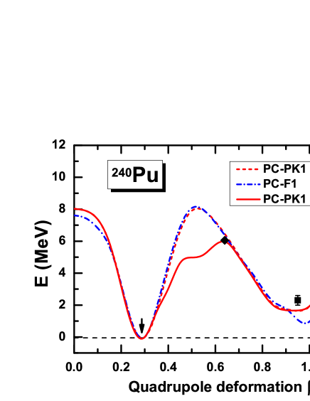
Figure 10: (Color online) The potential energy curves for ${}^{240}\rm Pu$ as functions of the quadrupole deformation $\beta_{2}$ in the calculations with PC-PK1. The dashed and solid lines correspond to the axial results and the triaxial results, i.e., the minima for each $\beta$ for the potential energy surface (PES) in the $\beta-\gamma$ plane, respectively. For comparison, the axially-symmetric result given by PC-F1 is also included as dot-dashed line. The data for the ground-state deformation Raman et al. (2001), the barrier height RIP (2006), and the energy of the fission isomer Bjørnholm and Lynn (1980) are respectively indicated by an arrow, a diamond, and a square. To guide the eyes, the diamond and square are respectively set at $\beta_{2}=0.64$ and $\beta_{2}=0.95$.

In Fig. 10, the potential energy curves for ${}^{240}\rm Pu$ as functions of the quadrupole deformation $\beta_{2}$ are shown. The dashed and solid lines correspond to the axially-symmetric and the triaxial calculations with PC-PK1, respectively. In the case of triaxial calculation, the solid line refers to the minima for each $\beta$ for the potential energy surface (PES) in the $\beta-\gamma$ plane. For comparison, the axially-symmetric result given by PC-F1 is also included.

It is found that the PC-PK1 provides not only a good description for the deformation of the ground state Raman et al. (2001) but also the energy difference between the ground-state and the shape isomeric state Bjørnholm and Lynn (1980). Furthermore, after including the triaxiality, as shown in Fig 10, the fission barrier given by PC-PK1 is in agreement with the empirical value RIP (2006). It should be noted that the pairing correlation plays an important role in the description of fission barrier. Discussion on the dependence of the fission barrier height on the pairing correlations can be found in Ref. Karatzikos et al. (2010).

VII Nuclear excited properties

As a test of the new parameter set PC-PK1 in the description of nuclear spectroscopic properties for low-lying excitation states, the collective excitation spectra and transition probabilities in ${}^{150}\rm Nd$ as well as the characteristic collective observables for Nd isotopes will be calculated starting from a five-dimensional collective Hamiltonian in which the parameters are determined by constrained self-consistent RMF calculations for triaxial shapes Nikšić et al. (2009); Li et al. (2009a, b).

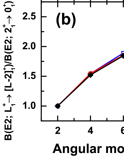
Figure 11: (Color online) The predicted excitation energies (upper panel) and $B(E2;L^{+}_{1}\rightarrow[L-2]^{+}_{1})$ values (lower panel) for the yrast states in ${}^{150}\rm Nd$ by PC-PK1 in comparison with data NND (http://www.nndc.bnl.gov/); LBN (http://ie.lbl.gov/toi.html) and those by DD-PC1 and PC-F1. The energies and $B(E2)$ values are respectively normalized to $E(2^{+}_{1})$ and $B(E2;2^{+}_{1}\rightarrow 0^{+}_{1})$.

In Fig. 11, the excitation energies and $B(E2;L^{+}_{1}\rightarrow[L-2]^{+}_{1})$ values for the yrast states in ${}^{150}\rm Nd$ predicted by PC-PK1 are shown in comparison with data NND (http://www.nndc.bnl.gov/); LBN (http://ie.lbl.gov/toi.html) and those by DD-PC1 and PC-F1. It can be seen that all the effective interactions provide similar excitation energies and intraband $B(E2)$ values for the yrast band and reproduce the data quite well.

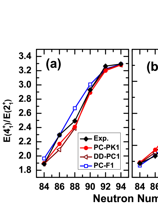
Figure 12: (Color online) The predicted characteristic collective observables $R_{4/2}=E(4^{+}_{1})/E(2^{+}_{1})$ and $B(E2;2^{+}_{1}\rightarrow 0^{+}_{1})$ (in W.u.) for Nd isotopes by PC-PK1 in comparison with data NND (http://www.nndc.bnl.gov/); LBN (http://ie.lbl.gov/toi.html) and those by DD-PC1 and PC-F1.

In Fig. 12, the characteristic collective observables $R_{4/2}=E(4^{+}_{1})/E(2^{+}_{1})$ and $B(E2;2^{+}_{1}\rightarrow 0^{+}_{1})$ for Nd isotopes given by PC-PK1 are shown in comparison with data NND (http://www.nndc.bnl.gov/); LBN (http://ie.lbl.gov/toi.html) and those by DD-PC1 and PC-F1. It is found that all the parameter sets reproduce the data quite well. In particular, the calculations reproduce in detail the rapid increase of $R_{4/2}$ and $B(E2)$ with the neutron number, i.e., from $R_{4/2}\sim 1.9$ and $B(E2)<30$ W.u. in near spherical ${}^{144}\rm Nd$ to $R_{4/2}\sim 3.3$ and $B(E2)>150$ W.u. in well-deformed ${}^{152}\rm Nd$.

It shows clearly that the new effective interaction PC-PK1 can provide a good description not only for the ground state properties in spherical and deformed nuclei but also for the nuclear spectroscopic properties of low-lying excitation states.

VIII Summary

In summary, a new parametrization PC-PK1 for the nuclear covariant energy density functional with nonlinear point-coupling interaction has been proposed by fitting to observables of 60 selected spherical nuclei, including the binding energies, charge radii and empirical pairing gaps. By scaling the coupling constants in PC-PK1 in accordance with the QCD-based Lagrangian, it is found that all the nine parameters are natural. The success of PC-PK1 has been illustrated through the description for infinite nuclear matter and finite nuclei including the ground-state and low-lying excited states.

For the spherical nuclei, PC-PK1 can provide better descriptions for the binding energies in comparison with DD-PC1, PC-F1, PC-LA, and NL3* sets. For neutron skin thicknesses, the DD-PC1 provides better description as compared with the other effective interactions due to its smaller symmetry energy at saturation density.

Taking Yb and U isotopes as examples, it is found that the PC-PK1 reproduces the deformations and their corresponding evolutions with neutron number quite well. After taking into account the rotational correction energy in the cranking approximation, the binding energies given by PC-PK1 are in very good agreement with data within 1 MeV, which indicates that PC-PK1 achieves the same quality as DD-PC1 in the description for deformed nuclei. Moreover, PC-PK1 provides good description for isospin dependence of binding energy along either the isotopic or the isotonic chains, which makes it reliable for application in exotic nuclei. It is noted that the rotational correction energy evaluated using the cranking approximation may differ from that using angular momentum projection.

Constrained calculations have also been performed for ${}^{240}\rm Pu$ in order to investigate the fission barrier. It is found that the PC-PK1 provides not only a good description for the deformation of the ground state Raman et al. (2001) but also the energy difference between the ground-state and the shape isomeric state Bjørnholm and Lynn (1980). Furthermore, after including the triaxiality, the fission barrier given by PC-PK1 is in agreement with the empirical value RIP (2006).

The predictive power of the PC-PK1 is also illustrated in the description for the collective excitation spectra and transition probabilities in ${}^{150}\rm Nd$ as well as the characteristic collective observables for Nd isotopes in a five-dimensional collective Hamiltonian in which the parameters are determined by constrained calculations for triaxial shapes. There are also many extensions of nuclear covariant energy density functional theory beyond mean-field using projection techniques Yao et al. (2009) and generator coordinate methods Nikšić et al. (2006); Yao et al. (2010b). More microscopic analysis of nuclear low-lying states in context of these frameworks with PC-PK1 is in progress.

The density-dependent parametrization DD-PC1 is determined mainly from the masses of deformed nuclei and the EOS of nuclear matter. However, the calculations of the rearrangement terms for the density-dependent parametrization can be nontrivial in some cases, in particular for RPA calculations. Here the nonlinear parametrization PC-PK1 has been optimized to the masses, charge radii and empirical pairing gaps for selected 60 spherical nuclei. It has been illustrated that the PC-PK1 can provide very good descriptions for both spherical and deformed nuclei. Therefore, the non-linear parametrization is very useful as it combines the simplicity with very good predictions for many nuclear properties.

Table 1: The point-coupling constants and pairing strengths of PC-PK1 set. The corresponding QCD-scaled coupling constants $c_{ln}$ are given in the last column as well.

Coupling Constant	Value	Dimension	$c_{ln}$
$~{}\alpha_{S}$	$-3.96291\times 10^{-4}$	${\rm MeV}^{-2}$	-1.695
$~{}\beta_{S}$	$8.6653\times 10^{-11}$	${\rm MeV}^{-5}$	1.628
$~{}\gamma_{S}$	$-3.80724\times 10^{-17}$	${\rm MeV}^{-8}$	-3.535
$~{}\delta_{S}$	$-1.09108\times 10^{-10}$	${\rm MeV}^{-4}$	-0.277
$~{}\alpha_{V}$	$2.6904\times 10^{-4}$	${\rm MeV}^{-2}$	1.151
$~{}\gamma_{V}$	$-3.64219\times 10^{-18}$	${\rm MeV}^{-8}$	-0.338
$~{}\delta_{V}$	$-4.32619\times 10^{-10}$	${\rm MeV}^{-4}$	-1.097
$~{}\alpha_{TV}$	$2.95018\times 10^{-5}$	${\rm MeV}^{-2}$	0.505
$~{}\delta_{TV}$	$-4.11112\times 10^{-10}$	${\rm MeV}^{-4}$	-4.171
$~{}V_{n}$	$-349.5$	${\rm MeV~{}fm}^{3}$
$~{}V_{p}$	$-330$	${\rm MeV~{}fm}^{3}$

Table 2: The calculated binding energies (in MeV) for selected spherical nuclei by PC-PK1 in comparison with the data Audi et al. (2003) and those by DD-PC1 Nikšić et al. (2008), PC-F1 Bürvenich et al. (2002), PC-LA Nikolaus et al. (1992), and NL3* Lalazissis et al. (2009). The bold-faced quantities denote that the experimental values of the corresponding nuclei are used in the parametrization fitting. The root mean square (rms) deviation $\displaystyle\Delta=\sum\limits_{i}^{N}\sqrt{(E_{i}^{\rm exp}-E_{i}^{\rm cal})^{2}/N}$ and the root of relative square (rrs) deviation $\displaystyle\delta=\sum\limits_{i}^{N}\sqrt{\frac{(E_{i}^{\rm exp}-E_{i}^{\rm cal})^{2}/(E_{i}^{\rm exp})^{2}}{N}}$ are respectively listed in the last two rows.

Nuclei	Exp.	PC-PK1	DD-PC1	PC-F1	PC-LA	NL3*
${}^{16}\rm O$	127.619	127.280	128.527	127.691	127.407	128.112
${}^{18}\rm O$	139.806	140.223	141.145	140.028	140.356	140.504
${}^{20}\rm O$	151.370	151.962	152.790	151.606	152.228	151.955
${}^{22}\rm O$	162.026	162.285	163.141	162.054	162.665	161.990
${}^{18}\rm Ne$	132.143	132.088	132.923	132.216	132.317	132.494
${}^{20}\rm Mg$	134.468	134.563	135.141	134.613	134.992	134.786
${}^{34}\rm Si$	283.429	284.727	285.967	285.067	283.989	283.236
${}^{36}\rm S$	308.714	308.374	309.305	308.973	307.221	306.086
${}^{38}\rm Ar$	327.342	327.107	328.691	328.540	326.755	325.379
${}^{36}\rm Ca$	281.360	281.412	281.878	282.001	280.454	279.579
${}^{38}\rm Ca$	313.122	313.230	314.501	314.415	312.901	311.669
${}^{40}\rm Ca$	342.052	343.060	345.113	345.041	343.202	341.578
${}^{42}\rm Ca$	361.896	363.142	365.143	364.411	363.685	361.547
${}^{44}\rm Ca$	380.960	381.915	383.967	382.748	382.789	380.246
${}^{46}\rm Ca$	398.769	399.451	401.668	400.060	400.627	397.718
${}^{48}\rm Ca$	415.990	415.492	417.973	416.085	416.969	413.616
${}^{50}\rm Ca$	427.490	426.937	428.660	427.302	426.883	424.445
${}^{42}\rm Ti$	346.905	348.024	349.848	349.701	348.626	346.539
${}^{50}\rm Ti$	437.781	436.445	437.761	436.171	437.223	434.389
${}^{56}\rm Ni$	483.992	483.669	481.447	480.758	481.826	481.058
${}^{58}\rm Ni$	506.458	503.636	502.587	501.646	502.623	501.342
${}^{72}\rm Ni$	613.169	614.875	617.071	614.646	614.486	612.561
${}^{84}\rm Se$	727.343	725.732	728.792	726.609	727.605	724.965
${}^{86}\rm Kr$	749.234	747.939	751.050	749.427	750.313	747.055
${}^{88}\rm Sr$	768.468	767.138	770.240	769.143	769.742	766.225
${}^{90}\rm Zr$	783.892	783.033	785.806	785.348	785.565	782.336
${}^{92}\rm Mo$	796.508	796.148	798.308	798.191	798.719	795.788
${}^{94}\rm Ru$	806.848	807.034	808.575	808.731	809.695	807.019
${}^{98}\rm Cd$	821.067	822.765	823.162	823.668	825.580	823.347
${}^{100}\rm Sn$	824.794	827.715	827.609	828.156	830.582	828.529
${}^{106}\rm Sn$	893.868	892.323	893.469	893.370	895.447	893.873
${}^{108}\rm Sn$	914.626	913.179	914.627	914.236	916.165	914.665
${}^{112}\rm Sn$	953.532	951.831	953.922	953.367	954.258	952.866
${}^{116}\rm Sn$	988.684	987.601	990.019	989.326	989.016	987.920
${}^{120}\rm Sn$	1020.546	1020.415	1022.902	1021.704	1020.767	1020.014
${}^{122}\rm Sn$	1035.529	1035.860	1038.417	1036.755	1035.794	1035.116
${}^{124}\rm Sn$	1049.963	1050.715	1053.402	1051.160	1050.327	1049.631
${}^{126}\rm Sn$	1063.889	1064.993	1067.877	1064.978	1064.381	1063.560
${}^{128}\rm Sn$	1077.346	1078.688	1081.835	1078.234	1077.945	1076.885
${}^{130}\rm Sn$	1090.293	1091.774	1095.253	1090.930	1090.993	1089.566
${}^{132}\rm Sn$	1102.851	1104.202	1108.096	1103.057	1103.484	1101.551
${}^{134}\rm Sn$	1109.235	1109.253	1112.253	1107.330	1106.707	1106.027
${}^{134}\rm Te$	1123.434	1124.205	1128.176	1124.193	1124.613	1122.859
${}^{136}\rm Xe$	1141.878	1142.621	1146.587	1143.601	1143.997	1142.480
${}^{138}\rm Ba$	1158.292	1159.381	1163.283	1161.245	1161.575	1160.331
${}^{140}\rm Ce$	1172.692	1174.054	1177.868	1176.722	1176.953	1175.954
${}^{142}\rm Nd$	1185.141	1185.938	1189.537	1189.138	1189.292	1188.002
${}^{144}\rm Sm$	1195.736	1195.736	1199.024	1199.353	1199.420	1198.079
${}^{146}\rm Gd$	1204.435	1203.712	1206.614	1207.635	1207.687	1206.449
${}^{148}\rm Dy$	1210.780	1209.974	1212.454	1214.117	1214.258	1213.186
${}^{150}\rm Er$	1215.331	1214.624	1216.686	1218.943	1219.236	1218.343
${}^{206}\rm Hg$	1621.049	1621.321	1623.820	1620.353	1616.956	1621.515
${}^{200}\rm Pb$	1576.354	1574.885	1577.817	1575.666	1575.769	1578.189
${}^{202}\rm Pb$	1592.187	1591.172	1594.139	1591.675	1591.240	1593.909
${}^{204}\rm Pb$	1607.506	1607.068	1610.026	1607.325	1606.187	1609.199
${}^{206}\rm Pb$	1622.324	1622.525	1625.385	1622.563	1620.490	1624.008
${}^{208}\rm Pb$	1636.430	1637.438	1640.008	1637.241	1633.865	1638.237
${}^{210}\rm Pb$	1645.552	1645.449	1648.272	1644.793	1641.484	1645.954
${}^{212}\rm Pb$	1654.514	1653.425	1656.428	1652.275	1648.887	1653.546
${}^{214}\rm Pb$	1663.291	1661.397	1664.481	1659.697	1656.073	1661.056
${}^{210}\rm Po$	1645.212	1646.703	1649.441	1647.760	1644.643	1648.995
${}^{212}\rm Rn$	1652.497	1654.632	1657.476	1656.863	1653.921	1658.319
${}^{214}\rm Ra$	1658.315	1661.172	1664.092	1664.512	1661.709	1666.174
${}^{216}\rm Th$	1662.689	1666.248	1669.244	1670.649	1667.967	1672.505
${}^{218}\rm U$	1665.648	1669.602	1672.733	1675.109	1672.491	1677.091
$\Delta$		1.33	3.09	2.60	2.64	2.88
$\delta$		0.18%	0.45%	0.32%	0.30%	0.34%

Table 2: (Continued).

Table 3: The calculated charge radii (in fm) for selected spherical nuclei by PC-PK1 in comparison with data De Vries et al. (1987); Nadjakov et al. (1994) and those by DD-PC1 Nikšić et al. (2008), PC-F1 Bürvenich et al. (2002), PC-LA Nikolaus et al. (1992), and NL3* Lalazissis et al. (2009). The bold-faced quantities denote that the experimental values of the corresponding nuclei are used in the parametrization fitting. The root mean square (rms) deviation $\displaystyle\Delta=\sum\limits_{i}^{N}\sqrt{(r_{i}^{\rm exp}-r_{i}^{\rm cal})^{2}/N}$ and the root of relative square (rrs) deviation $\displaystyle\delta=\sum\limits_{i}^{N}\sqrt{\frac{(r_{i}^{\rm exp}-r_{i}^{\rm cal})^{2}/(r_{i}^{\rm exp})^{2}}{N}}$ are respectively listed in the last two rows.

Nuclei	Exp.	PC-PK1	DD-PC1	PC-F1	PC-LA	NL3*
${}^{16}\rm O$	2.737	2.7677	2.7472	2.7633	2.7528	2.7352
${}^{40}\rm Ca$	3.4852	3.4815	3.4566	3.4777	3.4678	3.4704
${}^{42}\rm Ca$	3.5125	3.4805	3.4626	3.4778	3.4729	3.4672
${}^{44}\rm Ca$	3.5231	3.4826	3.4709	3.4809	3.4810	3.4672
${}^{46}\rm Ca$	3.5022	3.4865	3.4806	3.4860	3.4912	3.4693
${}^{48}\rm Ca$	3.4837	3.4890	3.4895	3.4906	3.5023	3.4705
${}^{50}\rm Ti$	3.573	3.5558	3.5696	3.5664	3.5868	3.5442
${}^{58}\rm Ni$	3.7827	3.7372	3.7761	3.7645	3.8065	3.7399
${}^{88}\rm Sr$	4.2036	4.2247	4.2231	4.2269	4.2379	4.2159
${}^{90}\rm Zr$	4.2720	4.2695	4.2664	4.2724	4.2847	4.2636
${}^{92}\rm Mo$	4.3170	4.3125	4.3140	4.3192	4.3333	4.3087
${}^{112}\rm Sn$	4.5957	4.5801	4.5894	4.5870	4.6044	4.5753
${}^{116}\rm Sn$	4.6257	4.6121	4.6174	4.6168	4.6307	4.6039
${}^{122}\rm Sn$	4.6633	4.6561	4.6579	4.6549	4.6728	4.6430
${}^{124}\rm Sn$	4.6739	4.6694	4.6714	4.6677	4.6864	4.6554
${}^{138}\rm Ba$	4.8348	4.8508	4.8511	4.8494	4.8667	4.8369
${}^{140}\rm Ce$	4.8774	4.8879	4.8879	4.8871	4.9037	4.8748
${}^{144}\rm Sm$	4.9525	4.9544	4.9521	4.9547	4.9676	4.9484
${}^{202}\rm Pb$	5.4772	5.4908	5.4869	5.4892	5.4996	5.4825
${}^{204}\rm Pb$	5.4861	5.5005	5.4962	5.4987	5.5112	5.4916
${}^{206}\rm Pb$	5.4946	5.5098	5.5049	5.5078	5.5200	5.5004
${}^{208}\rm Pb$	5.5046	5.5185	5.5129	5.5162	5.5279	5.5087
${}^{214}\rm Pb$	5.5622	5.5798	5.5711	5.5762	5.5813	5.5699
$\Delta$		0.019	0.019	0.017	0.023	0.022
$\delta$		0.53%	0.51%	0.45%	0.55%	0.60%

Table 4: The predicted saturation properties for nuclear matter by PC-PK1 in comparison with those by DD-PC1, PC-F1, PC-LA, NL3*, and PK1.

	PC-PK1	DD-PC1	PC-F1	PC-LA	NL3*	PK1
$\rho_{0}$ $\rm(fm^{-3})$	0.154	0.152	0.151	0.148	0.150	0.148
$E/A\rm(MeV)$	-16.12	-16.06	-16.17	-16.13	-16.31	-16.27
$M_{D}^{\ast}/M$	0.59	0.58	0.61	0.58	0.59	0.60
$M_{L}^{\ast}/M$	0.65	0.64	0.67	0.64	0.65	0.66
$K_{0}\rm(MeV)$	238	230	255	264	258	283
$E_{\rm sym}\rm(MeV)$	35.6	33	37.8	37.2	38.7	37.6
$L\rm(MeV)$	113	70	117	108	123	116
$K_{\rm asy}\rm(MeV)$	-583	-528	-627	-709	-630	-641

Figure 1: (Color online) The binding energy per nucleon $E/A$ for nuclear matter as a function of the baryon density $\rho_{B}$ given by PC-PK1, DD-PC1, PC-F1, PC-LA, NL3*, and PK1. The shaded area indicates the empirical value Brockmann and Machleidt (1990) and the filled diamonds present the microscopic results of the ab-initio variational calculation Akmal et al. (1998).

Figure 2: (Color online) Deviations of the calculated binding energies for Ca, Ni, Sn, and Pb isotopes by PC-PK1 from the data Audi et al. (2003) in comparison with those by DD-PC1, PC-F1, PC-LA, and NL3*.

Figure 3: (Color online) Same as Fig. 2 but for the N=20, N=50, N=82 and N=126 isotones.

Figure 4: (Color online) The calculated two-neutron separation energies for O, Ca, Ni, and Sn isotopes by PC-PK1 in comparison with data Audi et al. (2003) and those by DD-PC1, PC-F1, PC-LA, and NL3*.

Figure 5: (Color online) The calculated single-particle energies for ${}^{16}\rm O$ and ${}^{40}\rm Ca$ by PC-PK1 in comparison with data Isakov et al. (2002) and those by DD-PC1, PC-F1, PC-LA, and NL3*.

Figure 6: (Color online) Same as Fig. 5 but for ${}^{132}\rm Sn$ and ${}^{208}\rm Pb$.

Figure 7: (Color online) The calculated charge radii for Sn and Pb isotopes by the PC-PK1 in comparison with data De Vries et al. (1987); Nadjakov et al. (1994) and those by DD-PC1, PC-F1, PC-LA, and NL3*.

Figure 8: (Color online) The calculated neutron skin thicknesses for Sn isotopes and ${}^{208}\rm Pb$ by PC-PK1 in comparison with data Krasznahorkay et al. (2004); Clark et al. (2003) and those by DD-PC1, PC-F1, PC-LA, and NL3*. In the lower panel, the data for ${}^{208}\rm Pb$ deduced from antiprotonic atoms Trzcińska et al. (2001), polarized proton scattering Ray (1979); Hoffmann et al. (1981), elastic proton scattering Starodubsky and Hintz (1994), inelastic $\alpha$ scattering Krasznahorkay et al. (1994), and proton-nucleus elastic scattering Clark et al. (2003) are shown from left to right respectively.

Figure 9: (Color online) Deviations of the calculated binding energies from the data Audi et al. (2003) for Yb and U isotopes in axially deformed code by PC-PK1, DD-PC1 and PC-F1 (upper panel) as well as the corresponding calculated ground-state deformations in comparison with data Raman et al. (2001) (lower panel). The filled circles and squares in the upper panels correspond to the rotational corrected ones given by PC-PK1 and PC-F1 respectively.