Fate of non-Fermi liquid behavior in QED₃ at finite chemical potential

Abstract

The damping rate of two-dimensional massless Dirac fermions exhibit non-Fermi liquid behavior, $\propto\varepsilon^{1/2}$, due to gauge field at zero temperature and zero chemical potential. We study the fate of this behavior at finite chemical potential. We fist calculate explicitly the temporal and spatial components of vacuum polarization functions. The analytical expressions imply that the temporal component of gauge field develops a static screening length at finite chemical potential while the transverse component remains long-ranged owing to gauge invariance. We then calculate the fermion damping rate and show that the temporal gauge field leads to normal Fermi liquid behavior but the transverse gauge field leads to non-Fermi liquid behavior $\propto\varepsilon^{2/3}$ at zero temperature. This energy-dependence is more regular than $\propto\varepsilon^{1/2}$ and does not change as chemical potential varies.

I Introduction

The damping rate of fermions due to interaction with gauge fields is a physical quantity of broad interests. Studying this quantity can help us to judge whether an interacting fermion system displays non-Fermi liquid behavior or not. According to Landau, for any normal Fermi liquid to be stable, the fermion excitations must have a sufficiently long lifetime, which means that the fermion damping rate should vanish faster than energy $\varepsilon$ does as $\varepsilon\rightarrow 0$. At the low-energy regime, the fermion damping rate can be written in the form $\mathrm{Im}\Sigma(\varepsilon)\propto\varepsilon^{z}$. The system with exponent $z>1$ is a normal Fermi liquid, while system with $z\leq 1$ corresponds to a non-Fermi liquid. In conventional metals, the Coulomb interaction between electrons is always statically screened and can only lead to normal Fermi liquid behavior. Since the work of Holstein and coworkers Holstein , it has been known that the unscreened gauge field can give rise to non-Fermi liquid behavior. The unusual, non-Fermi liquid like, fermion damping rate caused by gauge field has attracted great attention in the past twenty years because an emergent gauge field is found to play important roles in a number of strongly correlated electron systems Varma2002 ; Reizer89 ; Lee89 ; Blok93 ; GanWong ; Polchinski ; Lee05 . In particle physics, this problem has also been discussed extensively in various gauge theories, including four-dimensional QCD Pisarski and four-dimensional QED Lebellac ; Blaizot .

Here we are particularly interested in the unusual properties of massless Dirac fermions. In some planar correlated electron systems, including $d$-wave high temperature superconductor Lee05 and graphene Castro , the valence band and conduction band touch only at discrete Dirac points. This is illustrated in Fig.1(a). The states in the lower valence band are fully occupied, while those in the upper conduction band are fully empty. The low-energy fermions excited from the lower band have a linear spectrum and hence can be described by massless Dirac fermions, which satisfy the relativistic Dirac equation Lee05 ; Castro . The interaction of massless Dirac fermions with an abelian gauge field in two spatial dimensions defines the three-dimensional quantum electrodynamics (QED₃). This field theory is usually studied by particle physicists as a toy model of QCD₄ since it is known to exhibit dynamical chiral symmetry breaking Appelquist88 and confinement Maris95 . In condensed matter physics, with proper modification, it serves as an effective low-energy theory of high temperature superconductors Affleck ; Kim97 ; Franz ; Kim99 and some spin-1/2 Kagome spin liquids Ran07 . In the realistic applications, chiral symmetry breaking and confinement in QED₃ correspond to the long-range Neel order in two-dimensional quantum Heisenberg antiferromagnet Kim99 .

Recently, we studied the damping rate of massless Dirac fermions due to gauge field in QED₃ in the absence of chiral symmetry breaking and confinement WangLiu . It diverges at both zero and finite temperatures when it is calculated using the straightforward perturbative expansion approach. Once the fermion damping effect and the dynamical screening effect of gauge field are self-consistently coupled, the fermion damping rate is then well-defined and behaves as $\mathrm{Im}\Sigma(\varepsilon)\propto\varepsilon^{1/2}$ at zero temperature WangLiu . This damping rate vanishes slower than $\varepsilon$ does in the $\varepsilon\rightarrow 0$ limit and thus displays non-Fermi liquid behavior.

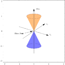
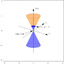
Figure 1: (a) The half-filling state with lower band being fully occupied and upper band fully empty. (b) At finite chemical potential $\mu$, the Fermi surface is finite.

This result was obtained in the so-called half-filling ground state depicted in Fig.1(a). In realistic condensed matter systems, the fermion density already can be continuously turned, either by chemical doping Lee05 or by adjusting a bias voltage Castro . When the fermion density grows from the Dirac point, a small but finite Fermi surface will emerge, as shown in Fig.1(b). To describe this process, the commonly used strategy is to introduce a chemical potential $\mu$, which defines the energy difference between the new Fermi surface and the Dirac point. The systems at zero and finite $\mu$ may have quite different properties. Indeed, there might be a quantum phase transition as the chemical potential varies Sachdev , with $\mu=0$ being the quantum critical point.

When the fermion density becomes sufficiently large, the interacting fermion system finally develops a large Fermi surface with low-energy fermionic excitations satisfying the non-relativistic Schrodinger equation. Historically, before the energy gap of high temperature cuprate superconductor was confirmed to have a $d$-wave symmetry, the fermion-gauge system with large Fermi surface had been studied intensively Varma2002 ; Lee89 ; Blok93 ; GanWong ; Polchinski ; Lee05 . The damping rate of non-relativistic fermions was calculated by various methods, including straightforward perturbation expansion Lee89 ; Blok93 , renormalization group approach GanWong , and Eliashberg theory Polchinski . Most of these studies found that $\mathrm{Im}\Sigma(\varepsilon)\propto\varepsilon^{2/3}$ at zero temperature. The exponent in the energy dependence of damping rate is quite different from that in QED₃ of massless Dirac fermions at $\mu=0$. The difference is presumably owing to the difference between a large Fermi surface and discrete Fermi points.

As $\mu$ grows from $\mu=0$ to a large value, the fermion damping rate will undergo a crossover from $\propto\varepsilon^{1/2}$ to $\propto\varepsilon^{2/3}$. A question naturally arises: Does the exponent $z$ appearing in $\varepsilon^{z}$ vary continuously from $1/2$ to $2/3$ or change abruptly at some critical value $\mu_{c}$?

In this paper, we study how the fermion damping rate varies with growing chemical potential $\mu$ by calculating the $\mu$-dependence of fermion self-energy. As usual, the gauge field is decoupled to longitudinal and transverse components. From the vacuum polarization functions at finite $\mu$, we know that the longitudinal component becomes short-ranged (massive) due to static Debye screening effect, but the transverse part remains long-ranged (massless) because of the gauge invariance. In this case, the transverse component of gauge field dominates and should be able to produce non-Fermi liquid behaviors. However, with increasing fermion density, the dynamical screening effect becomes stronger and hence may lead to less singular behavior than that at small $\mu$.

After explicit computation, we found that the transverse damping rate of Dirac fermions at zero temperature behaves as $\mathrm{Im}\Sigma_{\mathrm{T}}(\xi_{\mathbf{k}})\propto\mu^{-1/3}\xi_{\mathbf{k}}^{2/3}$, while the longitudinal contribution is $\mathrm{Im}\Sigma_{\mathrm{L}}(\xi_{\mathbf{k}})\propto\left(\xi_{\mathbf{k}}^{2}/\mu\right)\ln\left(\xi_{\mathbf{k}}/\mu\right)$, where $\xi_{\mathbf{k}}$ is the fermion energy in the on-shell approximation. Thus the total fermion damping rate is $\propto\mu^{-1/3}\xi_{\mathbf{k}}^{2/3}$, which is certainly non-Fermi liquid behavior. We also considered the fixed momentum approximation and obtained the same results, i.e., the fermion damping rate behaves as $\propto\mu^{-1/3}\varepsilon^{2/3}$ at zero temperature.

These results imply that the fermion damping rate suddenly becomes $\propto\varepsilon^{2/3}$ from $\propto\varepsilon^{1/2}$ once the chemical potential $\mu$ departs from zero. As $\mu$ grows, the energy-dependence of fermion damping rate does not change but its coefficient decreases. Therefore, although the Dirac fermions are always not well-defined in the sense of Landau quasiparticle, their lifetime increases slowly with growing fermion density.

The paper is organized as follows. The Lagrangian and some relevant quantities are defined In Sec. II. The full expressions of polarization functions from massless Dirac fermions at finite chemical potential are calculated in Sec. III and the fermion damping rate is calculated in Sec. IV. We summarize the results and briefly discuss the physical implications in Sec.V. The polarization functions at zero temperature are shown in the Appendix.

II Lagrangian and Feynman rules of QED₃ at finite chemical potential

We start from the following general Lagrangian of QED₃

$$\mathcal{L}=\sum_{i=1}^{N}\Psi_{i}^{\dagger}\left(\partial_{\tau}-\mu-iea_{0}-i\mathbf{\sigma}\cdot\left(\mathbf{\partial}-ie\mathbf{a}\right)\right)\Psi_{i}-\frac{1}{4}F^{2}.$$ (1)

This is the general Lagrangian for QED defined in (2+1)-dimensional space-time. As a well-defined relativistic quantum field theory, there is surely an explicit Maxwell term for the gauge field. As discussed in the Introduction, this is a very interesting and widely studied field theory in the context of particle physics. When applied to strongly correlated electron systems, it usually needs to be modified properly. If the effective QED₃ theory is derived by considering the phase fluctuations in underdoped high temperature superconductors, then normally the Maxwell term is present Franz . However, if the effective QED₃ theory is obtained by the slave-particle treatment of t-J model, there is no Maxwell term in the Lagrangian and the gauge field can have its dynamics only after integrating out the matter fields Affleck ; Kim97 . We will first consider the general action with the Maxwell term and briefly discuss the case without such term at the end of Sec.IV.

Here, we adopt the two-component representation of spinor field, with $\mathbf{\sigma}$ being the Pauli matrices. The Dirac fermion flavor $N$ is taken to be large so that we can use the $1/N$ expansion. The theory is defined at finite chemical potential $\mu$. The aim of this paper is to study how the fermion damping rate depends on $\mu$. For simplicity, we take $\hbar=c=k_{B}=1$ throughout the whole paper.

At finite temperature, the Matsubara propagator of massless Dirac fermion is

$$G_{0}\left(i\varepsilon_{n},\mathbf{k}\right)=\frac{1}{i\varepsilon_{n}+\mu-\mathbf{\sigma}\cdot\mathbf{k}},$$ (2)

where $\varepsilon_{n}=(2n+1)\pi T$ with $n$ being integer. After analytic continuation, the retarded propagator is

$$G_{0}(\varepsilon,\mathbf{k})=\frac{1}{\varepsilon+\mu-\mathbf{\sigma}\cdot\mathbf{k}+i\delta}.$$ (3)

At finite temperature, the temporal and spatial components of gauge field decouple and now it is convenient to work in the Coulomb gauge $k_{i}a_{i}=0$. In the imaginary time formalism, the propagator for the gauge field can now be written as

$$D_{00}\left(i\omega_{m},\mathbf{q}\right) = \frac{1}{|\mathbf{q}|^{2}+\Pi_{00}(i\omega_{m},\mathbf{q})},$$ (4)

$$D_{ij}\left(i\omega_{m},\mathbf{q}\right) = \left(\delta_{ij}-\frac{q_{i}q_{j}}{\mathbf{q}^{2}}\right)\frac{1}{|\mathbf{q}|^{2}\ +\omega_{m}^{2}+\Pi_{\bot}\left(i\omega_{m},\mathbf{q}\right)},$$

(5)

where $\omega_{m}=2m\pi T$ for bosonic modes with $m$ being integers. The vacuum polarization functions $\Pi_{00}(\omega_{m},\mathbf{q})$ and $\Pi_{\bot}(\omega_{m},\mathbf{q})$ come from the one-loop bubble diagram of Dirac fermions to the leading order of $1/N$ expansion. In particular, the polarization function appearing in the spatial component is given by

$$\Pi_{\bot}(i\omega_{m},\mathbf{q})=\Pi_{ii}(i\omega_{m},\mathbf{q})-\frac{\omega_{m}^{2}}{\mathbf{q}^{2}}\Pi_{00}(i\omega_{m},\mathbf{q}).$$ (6)

The functions $\Pi_{00}(i\omega_{m},\mathbf{q})$ and $\Pi_{ii}(i\omega_{m},\mathbf{q})$ are defined as

$$\Pi_{00}(i\omega_{m},\mathbf{q}) = -Ne^{2}T\sum_{i\varepsilon_{n}}\int\frac{d^{2}k}{(2\pi)^{2}}$$ (7)

$$\times\mathrm{Tr}[G_{0}(i\varepsilon_{n},\mathbf{k})G_{0}(i\varepsilon_{n}+i\omega_{m},\mathbf{q}+\mathbf{k})],$$

$$\Pi_{ii}(i\omega_{m},\mathbf{q}) = Ne^{2}T\sum_{i\varepsilon_{n}}\int\frac{d^{2}k}{(2\pi)^{2}}$$

$$\times\mathrm{Tr}[\sigma_{i}G_{0}(i\varepsilon_{n},\mathbf{k})\sigma_{i}G_{0}(i\varepsilon_{n}+i\omega_{m},\mathbf{q}+\mathbf{k})].$$

When we calculate the fermion damping rate, we need the real and imaginary parts of the retarded polarization functions. They can be obtained by straightforward computation, which will be given in the next section.

The fermion damping rate can be calculated by the standard finite temperature field theory technique Giuliani . To the lowest order of $1/N$ expansion, the self-energy of Dirac fermion is given by

$$\Sigma(i\varepsilon_{n},\mathbf{k})=\Sigma_{\mathrm{L}}(i\varepsilon_{n},\mathbf{k})+\Sigma_{\mathrm{T}}(i\varepsilon_{n},\mathbf{k}),$$ (9)

where

$$\Sigma_{\mathrm{L}}(i\varepsilon_{n},\mathbf{k}) = -e^{2}T\sum_{i\omega_{m}}\frac{1}{2}\mathrm{Tr}\Big{[}\mathbf{1}\cdot\int\frac{d^{2}\mathbf{q}}{(2\pi)^{2}}$$ (10)

$$\times G_{0}(i\varepsilon_{n}+i\omega_{m},\mathbf{k+q})D_{00}(i\omega_{m},\mathbf{q})\Big{]},$$

$$\Sigma_{\mathrm{T}}(i\varepsilon_{n},\mathbf{k}) = e^{2}T\sum_{i\omega_{m}}\frac{1}{2}\mathrm{Tr}\Big{[}\mathbf{1}\cdot\int\frac{d^{2}\mathbf{q}}{(2\pi)^{2}}$$

$$\times\sigma_{i}G_{0}(i\varepsilon_{n}+i\omega_{m},\mathbf{k+q})\sigma_{j}D_{ij}(i\omega_{m},\mathbf{q})\Big{]},$$

are the contributions from the longitudinal and transverse components of the gauge field, respectively. The damping rate of massless Dirac fermion will be obtained by making analytic continuation, $i\varepsilon_{n}\rightarrow\varepsilon+i\delta$, as

$$\Sigma(\varepsilon,\mathbf{k})=\Sigma_{\mathrm{L}}(\varepsilon,\mathbf{k})+\Sigma_{\mathrm{T}}(\varepsilon,\mathbf{k}),$$ (12)

and then taking the imaginary part, $\mathrm{Im}\Sigma(\varepsilon,\mathbf{k})$.

When the Fermi level lies exactly at the Dirac point, the states below the point are all occupied while the states beyond it are all empty (see Fig.1(a)). In this state, the chemical potential is usually defined as zero, $\mu=0$. In a previous paper, we studied the Dirac fermion damping rate and found that it behaves as $\mathrm{Im}\Sigma(\varepsilon)\propto\varepsilon^{1/2}$ at zero temperature, which is a typical non-Fermi liquid behavior. Once the fermion density increases starting from the Dirac point, the system develops a finite chemical potential $\mu$ (Fig.1(b)). Now the system has a finite but small Fermi surface. The density of states of fermions at the Fermi level has a finite quantity. Therefore, at finite $\mu$, the gauge field may lead to very different behaviors for the fermion damping rate.

In order to know how fermion damping rate varies with $\mu$, we will explicitly calculate the fermion self-energy. To this end, we first calculate the polarization functions $\Pi_{00}(i\omega_{m},\mathbf{q})$ and $\Pi_{ii}(i\omega_{m},\mathbf{q})$.

III Computation of polarization functions

The polarization functions contributed by the massless Dirac fermions deserve careful exploration since they determine or are directly related to many important physical quantities. For instance, the dynamical screening effect of collective particle-hole excitations on the gauge or Coulomb interaction between Dirac fermions can only be studied by the polarization functions. Physically, such effect describes the damping of gauge boson in the many-body background composed of massless Dirac fermions. In addition, according to the Kubo formula in transport theory, various conductivities are all given by their corresponding current-current correlation functions, which in form are analogous to the polarization functions.

In this section, we briefly outline the computational steps and present the complete expressions for polarization functions $\Pi_{00}$ and $\Pi_{\bot}$ in the presence of finite chemical potential at both zero and finite temperature. The analytical expressions will be useful to any work that relies on the properties of polarization functions of two-dimensional Dirac fermions.

III.1 Temporal component $\Pi_{00}(\omega,\mathbf{q},T)$

To calculate the temporal component of polarization function $\Pi_{00}(i\omega_{m},\mathbf{q})$, we first introduce the spectral representation

$$G_{0}\left(i\varepsilon_{n},\mathbf{k}\right)=-\int_{-\infty}^{+\infty}\frac{d\omega_{1}}{\pi}\frac{\mathrm{Im}\left[G_{0}(\omega_{1},\mathbf{k})\right]}{i\varepsilon_{n}-\omega_{1}}$$ (13)

and then sum over the frequency, which yields

$$\Pi_{00}\left(i\omega_{m},\mathbf{q}\right) = -Ne^{2}\int\frac{d^{2}\mathbf{k}}{(2\pi)^{2}}\mathrm{Tr}\left[\int_{-\infty}^{+\infty}\frac{d\omega_{1}}{\pi}\mathrm{Im}\left[G_{0}(\omega_{1},\mathbf{k})\right]\int_{-\infty}^{+\infty}\frac{d\omega_{2}}{\pi}\mathrm{Im}\left[G_{0}(\omega_{2},\mathbf{k+q})\right]\right]$$ (14)

$$\times\frac{n_{F}(\omega_{1})-n_{F}(\omega_{2})}{\omega_{1}-\omega_{2}+i\omega_{m}}.$$

It is convenient to make the analytic continuation $i\omega_{m}\rightarrow\omega+i\delta$ at this stage:

$$\frac{1}{\omega_{1}-\omega_{2}+i\omega_{n}}\rightarrow\frac{1}{\omega_{1}-\omega_{2}+\omega+i\delta}=P\frac{1}{\omega_{1}-\omega_{2}+\omega}-i\pi\delta(\omega_{1}-\omega_{2}+\omega).$$ (15)

The imaginary part of the retarded polarization function is

$$\mathrm{Im}\Pi_{00}(\omega,\mathbf{q}) = N\pi e^{2}\int\frac{d^{2}\mathbf{k}}{(2\pi)^{2}}\mathrm{Tr}\left[\int_{-\infty}^{+\infty}\frac{d\omega_{1}}{\pi}\mathrm{Im}\left[G_{0}(\omega_{1},\mathbf{k})\right]\int_{-\infty}^{+\infty}\frac{d\omega_{2}}{\pi}\mathrm{Im}\left[G_{0}\left(\omega_{2},\mathbf{k+q}\right)\right]\right]$$ (16)

$$\times\left[n_{F}(\omega_{1})-n_{F}(\omega_{2})\right]\delta\left(\omega_{1}-\omega_{2}+\omega\right).$$

Here the imaginary part of retarded fermion Green function is given by

$$\mathrm{Im}\left[G_{0}(\omega,\mathbf{k})\right] = \mathrm{Im}\left[\frac{1}{\omega+\mu-\mathbf{\sigma}\cdot\mathbf{k}+i\delta}\right]$$ (17)

$$= \mathrm{Im}\left[\frac{\omega+\mu+\mathbf{\sigma}\cdot\mathbf{k}}{\left(\omega+\mu\right)^{2}-\left|\mathbf{k}\right|^{2}+i\mathrm{sgn}\left(\omega+\mu\right)\delta}\right]$$

$$= -\pi\mathrm{sgn}(\omega+\mu)\left(\omega+\mu+\mathbf{\sigma\cdot k}\right)\delta\left((\omega+\mu)^{2}-|\mathbf{k}|^{2}\right)$$

$$= -\pi\mathrm{sgn}(\omega+\mu)\left(\omega+\mu+\mathbf{\sigma\cdot k}\right)\frac{1}{2|\mathbf{k}|}\left[\delta\left(\omega+\mu+|\mathbf{k}|\right)+\delta\left(\omega+\mu-|\mathbf{k}|\right)\right].$$

After tedious computation, we finally have

$$\mathrm{Im}\Pi_{00}\left(\omega,\mathbf{q},T\right)\\ =\left\{\begin{array}[]{ll}\sum_{\alpha=\pm 1}\mathrm{sgn}(\omega)\frac{Ne^{2}}{8\pi}\frac{|\mathbf{q}|^{2}}{\sqrt{\omega^{2}-|\mathbf{q}|^{2}}}\int_{-1}^{1}dx\sqrt{1-x^{2}}\left[\delta_{\alpha,1}-\frac{1}{1+e^{\frac{|\mathbf{q}|x+|\omega|-2\alpha\mu}{2T}}}\right]\\ \hskip 256.0748pt\mbox{when}\qquad|\omega|>|\mathbf{q}|,\\ \\ \sum_{\alpha=\pm 1}\mathrm{sgn}(\omega)\frac{Ne^{2}}{8\pi}\frac{|\mathbf{q}|^{2}}{\sqrt{|\mathbf{q}|^{2}-\omega^{2}}}\int_{1}^{+\infty}dx\left[\frac{\sqrt{x^{2}-1}}{1+e^{\frac{|\mathbf{q}|x-|\omega|-2\alpha\mu}{2T}}}-\frac{\sqrt{x^{2}-1}}{1+e^{\frac{|\mathbf{q}|x+|\omega|-2\alpha\mu}{2T}}}\right]\\ \hskip 256.0748pt\mbox{when}\quad|\omega|<|\mathbf{q}|.\end{array}\right.$$ (18)

We now calculate the real part of temporal component of polarization function. The whole computation is much more complicated than the imaginary part. From Eq.(14) and Eq.(15), we have

$$\mathrm{Re}\Pi_{00}\left(\omega,\mathbf{q},T\right) = -Ne^{2}P\int\frac{d^{2}\mathbf{k}}{(2\pi)^{2}}\mathrm{Tr}\left[\int_{-\infty}^{+\infty}\frac{d\omega_{1}}{\pi}\mathrm{Im}\left[G_{0}\left(\omega_{1},\mathbf{k}\right)\right]\int_{-\infty}^{+\infty}\frac{d\omega_{2}}{\pi}\mathrm{Im}\left[G_{0}(\omega_{2},\mathbf{k+q})\right]\right]$$ (19)

$$\times\frac{n_{F}(\omega_{1})-n_{F}(\omega_{2})}{\omega_{1}-\omega_{2}+\omega}$$

$$= -Ne^{2}\int\frac{d^{2}\mathbf{k}}{(2\pi)^{2}}\mathrm{Tr}\left[\int_{-\infty}^{+\infty}\frac{d\omega_{1}}{\pi}\mathrm{Im}\left[G_{0}\left(\omega_{1},\mathbf{k}\right)\right]n_{F}(\omega_{1})P\int_{-\infty}^{+\infty}\frac{d\omega_{2}}{\pi}\frac{\mathrm{Im}\left[G_{0}(\omega_{2},\mathbf{k+q})\right]}{\omega_{1}+\omega-\omega_{2}}\right]$$

$$-Ne^{2}\int\frac{d^{2}\mathbf{k}}{(2\pi)^{2}}\mathrm{Tr}\left[\int_{-\infty}^{+\infty}\frac{d\omega_{2}}{\pi}\mathrm{Im}\left[G_{0}(\omega_{2},\mathbf{k+q})\right]n_{F}(\omega_{2})P\int_{-\infty}^{+\infty}\frac{d\omega_{1}}{\pi}\frac{\mathrm{Im}\left[G_{0}(\omega_{1},\mathbf{k})\right]}{\omega_{2}-\omega-\omega_{1}}\right].$$

Using the Krames-Kronig relation

$$\mathrm{Re}\left[G_{0}(\omega,\mathbf{k})\right]=-P\int_{-\infty}^{+\infty}\frac{d\omega^{\prime}}{\pi}\frac{\mathrm{Im}\left[G_{0}(\omega^{\prime},\mathbf{k})\right]}{\omega-\omega^{\prime}},$$ (20)

the above expression can now be converted to

$$\mathrm{Re}\Pi_{00}(\omega,\mathbf{q},T) = Ne^{2}\int\frac{d^{2}\mathbf{k}}{(2\pi)^{2}}\int_{-\infty}^{+\infty}\frac{d\omega_{1}}{\pi}n_{F}(\omega_{1})\mathrm{Tr}\left[\mathrm{Im}\left[G_{0}(\omega_{1},\mathbf{k})\right]\mathrm{Re}\left[G_{0}(\omega_{1}+\omega,\mathbf{k+q})\right]\right]$$ (21)

$$+Ne^{2}\int\frac{d^{2}\mathbf{k}}{(2\pi)^{2}}\int_{-\infty}^{+\infty}\frac{d\omega_{1}}{\pi}n_{F}(\omega_{1})\mathrm{Tr}\left[\mathrm{Im}\left[G_{0}(\omega_{1},\mathbf{k+q})\right]\mathrm{Re}\left[G_{0}(\omega_{1}-\omega,\mathbf{k})\right]\right],$$

where

$$\mathrm{Re}G_{0}\left(\omega,\mathbf{k}\right)=\left(\omega+\mu+\mathbf{\sigma\cdot k}\right)P\frac{1}{\left(\omega+\mu\right)^{2}-\left|\mathbf{k}\right|^{2}}.$$ (22)

From this equation, we obtain the following expression:

$$\mathrm{Re}\Pi_{00}\left(\omega,\mathbf{q},T\right)=-\frac{Ne^{2}}{2\pi}\int_{0}^{+\infty}d|\mathbf{k}|+\left\{\begin{array}[]{ll}\sum_{\alpha=\pm 1}\left\{\frac{Ne^{2}T\ln\left(1+e^{\frac{\alpha\mu}{T}}\right)}{2\pi}-\frac{Ne^{2}}{8\pi}\frac{|\mathbf{q}|^{2}}{\sqrt{\omega^{2}-|\mathbf{q}|^{2}}}\int_{1}^{+\infty}dx\sqrt{x^{2}-1}\right.\\ \left.\times\left[\frac{1}{1+e^{\frac{\left||\mathbf{q}|x-|\omega|\right|-2\alpha\mu}{2T}}}-\frac{1}{1+e^{\frac{|\mathbf{q}|x+|\omega|-2\alpha\mu}{2T}}}\right]\right\}\\ \hskip 142.26378pt\mbox{when}\quad|\omega|>|\mathbf{q}|,\\ \\ \sum_{\alpha\pm 1}\left\{\frac{Ne^{2}T\ln\left(1+e^{\frac{\alpha\mu}{T}}\right)}{2\pi}+\frac{Ne^{2}}{8\pi}\frac{|\mathbf{q}|^{2}}{\sqrt{|\mathbf{q}|^{2}-\omega^{2}}}\int_{-1}^{1}dx\sqrt{1-x^{2}}\right.\\ \left.\times\left[\delta_{\alpha,1}-\frac{1}{1+e^{\frac{\left||\mathbf{q}|x+|\omega|\right|-2\alpha\mu}{2T}}}\right]\right\}\\ \hskip 142.26378pt\mbox{when}\quad|\omega|<|\mathbf{q}|.\end{array}\right.$$ (23)

Notice there appears a divergent term

$$I_{\mathrm{Singular}}=-\frac{Ne^{2}}{2\pi}\int_{0}^{+\infty}d|\mathbf{k}|.$$ (24)

To remove this divergence, here we employ the regularization scheme that was proposed in Franz02 . This scheme states that the gauge field must remain massless so that it should satisfy

$$\Pi_{\mu\nu}\left(\omega\rightarrow 0,|\mathbf{q}|\rightarrow 0,\mu=0,T=0\right)=0.$$ (25)

Now the polarization function can be re-defined as

$$\Pi_{\mu\nu}(\omega,\mathbf{q},T)-\Pi_{\mu\nu}\left(\omega\rightarrow 0,|\mathbf{q}|\rightarrow 0,\mu=0,T=0\right).$$ (26)

After this regularization, the singular term can be simply dropped from $\mathrm{Re}\Pi_{00}\left(\omega,\mathbf{q},T\right)$.

III.2 Transverse component $\Pi_{\bot}\left(\omega,\mathbf{q},T\right)$

Proceeding as we have done in the above, we found that the imaginary and real parts of $\Pi_{ii}\left(\omega,\mathbf{q},T\right)$ have the expressions:

$$\mathrm{Im}\Pi_{ii}\left(\omega,\mathbf{q},T\right)=\left\{\begin{array}[]{ll}\sum_{\alpha=\pm 1}\left\{-\mathrm{sgn}(\omega)\frac{Ne^{2}}{8\pi}\frac{|\mathbf{q}|^{2}}{\sqrt{\omega^{2}-|\mathbf{q}|^{2}}}\int_{-1}^{1}dx\sqrt{1-x^{2}}\left[\delta_{\alpha,1}-\frac{1}{1+e^{\frac{|\mathbf{q}|x+|\omega|-2\alpha\mu}{2T}}}\right]\right.\\ \left.-\mathrm{sgn}(\omega)\frac{Ne^{2}}{8\pi}\sqrt{\omega^{2}-|\mathbf{q}|^{2}}\int_{-1}^{1}dx\frac{1}{\sqrt{1-x^{2}}}\left[\delta_{\alpha,1}-\frac{1}{1+e^{\frac{|\mathbf{q}|x+|\omega|-2\alpha\mu}{2T}}}\right]\right\}\\ \hskip 256.0748pt\mbox{when}\qquad|\omega|>|\mathbf{q}|,\\ \\ \sum_{\alpha=\pm 1}\left\{-\mathrm{sgn}(\omega)\frac{Ne^{2}}{8\pi}\frac{|\mathbf{q}|^{2}}{\sqrt{|\mathbf{q}|^{2}-\omega^{2}}}\int_{1}^{+\infty}dx\left[\frac{\sqrt{x^{2}-1}}{1+e^{\frac{|\mathbf{q}|x-|\omega|-2\alpha\mu}{2T}}}-\frac{\sqrt{x^{2}-1}}{1+e^{\frac{|\mathbf{q}|x+|\omega|-2\alpha\mu}{2T}}}\right]\right.\\ \left.-\mathrm{sgn}(\omega)\frac{Ne^{2}}{8\pi}\sqrt{|\mathbf{q}|^{2}-\omega^{2}}\int_{1}^{+\infty}dx\frac{1}{\sqrt{x^{2}-1}}\left[\frac{1}{1+e^{\frac{|\mathbf{q}|x-|\omega|-2\alpha\mu}{2T}}}-\frac{1}{1+e^{\frac{|\mathbf{q}|x+|\omega|-2\alpha\mu}{2T}}}\right]\right\}\\ \hskip 256.0748pt\mbox{when}\qquad|\omega|<|\mathbf{q}|.\end{array}\right.$$

$$\mathrm{Re}\Pi_{ii}\left(\omega,\mathbf{q},T\right)=\left\{\begin{array}[]{ll}\sum_{\alpha=\pm 1}\left\{\frac{Ne^{2}}{8\pi}\frac{|\mathbf{q}|^{2}}{\sqrt{\omega^{2}-|\mathbf{q}|^{2}}}\int_{1}^{+\infty}dx\left[\frac{\sqrt{x^{2}-1}}{1+e^{\frac{\left||\mathbf{q}|x-|\omega|\right|-2\alpha\mu}{2T}}}-\frac{\sqrt{x^{2}-1}}{1+e^{\frac{|\mathbf{q}|x+|\omega|-2\alpha\mu}{2T}}}\right]\right.\\ \\ \left.-\frac{Ne^{2}}{8\pi}\sqrt{\omega^{2}-|\mathbf{q}|^{2}}\int_{1}^{+\infty}dx\frac{1}{\sqrt{x^{2}-1}}\left[\frac{1}{1+e^{\frac{\left||\mathbf{q}|x-|\omega|\right|-2\alpha\mu}{2T}}}-\frac{1}{1+e^{\frac{|\mathbf{q}|x+|\omega|-2\alpha\mu}{2T}}}\right]\right\}\\ \hskip 256.0748pt\mbox{when}\quad|\omega|>|\mathbf{q}|,\\ \\ \sum_{\alpha=\pm 1}\left\{-\frac{Ne^{2}}{8\pi}\frac{|\mathbf{q}|^{2}}{\sqrt{|\mathbf{q}|^{2}-\omega^{2}}}\int_{-1}^{1}dx\sqrt{1-x^{2}}\left[\delta_{\alpha,1}-\frac{1}{1+e^{\frac{\left||\mathbf{q}|x+|\omega|\right|-2\alpha\mu}{2T}}}\right]\right.\\ \\ \left.+\frac{Ne^{2}}{8\pi}\sqrt{|\mathbf{q}|^{2}-\omega^{2}}\int_{-1}^{1}dx\frac{1}{\sqrt{1-x^{2}}}\left[\delta_{\alpha,1}-\frac{1}{1+e^{\frac{\left||\mathbf{q}|x+|\omega|\right|-2\alpha\mu}{2T}}}\right]\right\}\\ \hskip 256.0748pt\mbox{when}\quad|\omega|<|\mathbf{q}|.\end{array}\right.$$ (27)

According to Eq.(6), the retarded transverse polarization function is decomposed as

$$\Pi_{\bot}(\omega,\mathbf{q},T)=\Pi_{ii}(\omega,\mathbf{q},T)+\frac{\omega^{2}}{|\mathbf{q}|^{2}}\Pi_{00}(\omega,\mathbf{q},T),$$ (28)

which can be written more explicitly as

$$\mathrm{Im}\Pi_{\bot}(\omega,\mathbf{q},T) = \mathrm{Im}\Pi_{ii}(\omega,\mathbf{q},T)+\frac{\omega^{2}}{|\mathbf{q}|^{2}}\mathrm{Im}\Pi_{00}(\omega,\mathbf{q},T),$$ (29)

$$\mathrm{Re}\Pi_{\bot}(\omega,\mathbf{q},T) = \mathrm{Re}\Pi_{ii}(\omega,\mathbf{q},T)+\frac{\omega^{2}}{|\mathbf{q}|^{2}}\mathrm{Re}\Pi_{00}(\omega,\mathbf{q},T).$$ (30)

Using the results presented above, it is easy to get that

$$\mathrm{Im}\Pi_{\bot}(\omega,\mathbf{q},T)=\left\{\begin{array}[]{ll}-\sum_{\alpha=\pm 1}\mathrm{sgn}(\omega)\frac{Ne^{2}}{8\pi}\sqrt{\omega^{2}-|\mathbf{q}|^{2}}\int_{-1}^{1}dx\frac{x^{2}}{\sqrt{1-x^{2}}}\left[\delta_{\alpha,1}-\frac{1}{1+e^{\frac{|\mathbf{q}|x+|\omega|-2\alpha\mu}{2T}}}\right]\\ \hskip 256.0748pt\mbox{when}\qquad|\omega|>|\mathbf{q}|,\\ \\ -\sum_{\alpha=\pm 1}\mathrm{sgn}(\omega)\frac{Ne^{2}}{8\pi}\sqrt{|\mathbf{q}|^{2}-\omega^{2}}\int_{1}^{+\infty}dx\frac{x^{2}}{\sqrt{x^{2}-1}}\left[\frac{1}{1+e^{\frac{|\mathbf{q}|x-|\omega|-2\alpha\mu}{2T}}}\right.\\ \left.-\frac{1}{1+e^{\frac{|\mathbf{q}|x+|\omega|-2\alpha\mu}{2T}}}\right]\\ \hskip 256.0748pt\mbox{when}\qquad|\omega|<|\mathbf{q}|.\end{array}\right.$$ (31)

$$\mathrm{Re}\Pi_{\bot}(\omega,\mathbf{q},T)=\left\{\begin{array}[]{ll}\sum_{\alpha=\pm 1}\left\{\frac{Ne^{2}T\ln\left(1+e^{\frac{\alpha\mu}{T}}\right)}{2\pi}\frac{\omega^{2}}{|\mathbf{q}|^{2}}-\frac{Ne^{2}}{8\pi}\sqrt{\omega^{2}-|\mathbf{q}|^{2}}\int_{1}^{+\infty}dx\frac{x^{2}}{\sqrt{x^{2}-1}}\right.\\ \left.\times\left[\frac{1}{1+e^{\frac{\left||\mathbf{q}|x-|\omega|\right|-2\alpha\mu}{2T}}}-\frac{1}{1+e^{\frac{|\mathbf{q}|x+|\omega|-2\alpha\mu}{2T}}}\right]\right\}\\ \hskip 256.0748pt\mbox{when}\qquad|\omega|>|\mathbf{q}|,\\ \\ \sum_{\alpha=\pm 1}\left\{\frac{Ne^{2}T\ln\left(1+e^{\frac{\alpha\mu}{T}}\right)}{2\pi}\frac{\omega^{2}}{|\mathbf{q}|^{2}}+\frac{Ne^{2}}{8\pi}\sqrt{|\mathbf{q}|^{2}-\omega^{2}}\int_{-1}^{1}dx\frac{x^{2}}{\sqrt{1-x^{2}}}\right.\\ \left.\times\left[\delta_{\alpha,1}-\frac{1}{1+e^{\frac{\left||\mathbf{q}|x+|\omega|\right|-2\alpha\mu}{2T}}}\right]\right\}\\ \hskip 256.0748pt\mbox{when}\qquad|\omega|<|\mathbf{q}|.\end{array}\right.$$ (32)

IV Fermion damping rate at zero temperature

In this section, we calculate the fermion damping rate at zero temperature. We first consider the transverse contribution of gauge field to fermion damping rate. To do this, we will substitute the transverse gauge propagator Eq.(5) to transvrese self-energy function Eq.(LABEL:eqn:SelfEnergyT). Here, it is convenient to introduce the following spectral representations:

$$G_{0}\left(i\varepsilon_{n}+i\omega_{m},\mathbf{k+q}\right) = -P\int_{-\infty}^{+\infty}\frac{d\omega_{1}}{\pi}\frac{\mathrm{Im}\left[G_{0}\left(\omega_{1},\mathbf{k+q}\right)\right]}{i\varepsilon_{n}+i\omega_{m}-\omega_{1}},$$ (33)

$$\frac{1}{|\mathbf{q}|^{2}+\omega_{m}^{2}+\Pi_{\bot}\left(i\omega_{m},|\mathbf{q}|\right)} = -P\int_{-\infty}^{+\infty}\frac{d\omega_{2}}{\pi}\frac{1}{i\omega_{m}-\omega_{2}}\mathrm{Im}\left[\frac{1}{|\mathbf{q}|^{2}-\omega_{2}^{2}-i\mathrm{sgn}\left(\omega_{2}\right)\delta+\Pi_{\bot}\left(\omega_{2},|\mathbf{q}|\right)}\right].$$ (34)

After carrying out the summation over $\omega_{m}$, we can get

$$\Sigma_{\mathrm{T}}\left(i\varepsilon_{n},\mathbf{k}\right) = -e^{2}\frac{1}{2}\mathrm{Tr}\Bigg{[}\mathbf{1}\cdot\int\frac{d^{2}\mathbf{q}}{\left(2\pi\right)^{2}}\sigma_{i}\int_{-\infty}^{+\infty}\frac{d\omega_{1}}{\pi}\mathrm{Im}\left[G_{0}\left(\omega_{1},\mathbf{k+q}\right)\right]\sigma_{j}\left(\delta_{ij}-q_{i}q_{j}/|\mathbf{q}|^{2}\right)\int_{-\infty}^{+\infty}\frac{d\omega_{2}}{\pi}$$ (35)

$$\times\mathrm{Im}\left[\frac{1}{|\mathbf{q}|^{2}-\omega_{2}^{2}-i\mathrm{sgn}\left(\omega_{2}\right)\delta+\Pi_{\bot}\left(\omega_{2},|\mathbf{q}|\right)}\right]\frac{n_{B}\left(\omega_{2}\right)+n_{F}\left(\omega_{1}\right)}{i\varepsilon_{n}+\omega_{2}-\omega_{1}}\Bigg{]}.$$

After analytic continuation $i\varepsilon_{n}\rightarrow\varepsilon+i\delta$, we have

$$\frac{1}{i\varepsilon_{n}+\omega_{2}-\omega_{1}}\rightarrow\frac{1}{\varepsilon+\omega_{2}-\omega_{1}+i\delta}=P\frac{1}{\varepsilon+\omega_{2}-\omega_{1}}-i\pi\delta\left(\varepsilon+\omega_{2}-\omega_{1}\right),$$ (36)

and the imaginary part of fermion self-energy becomes

$$\mathrm{Im}\Sigma_{\mathrm{T}}(\varepsilon,\mathbf{k},T) = -e^{2}\int\frac{d^{2}\mathbf{q}}{(2\pi)^{2}}\mathrm{Im}\left[\frac{1}{|\mathbf{q}|^{2}-(|\mathbf{k+q}|-\mu-\varepsilon)^{2}-i\delta\mathrm{sgn}(|\mathbf{k+q}|-\mu-\varepsilon)+\Pi_{\bot}(|\mathbf{k+q}|-\mu-\varepsilon,|\mathbf{q}|)}\right]$$ (37)

$$\times\left[n_{B}(|\mathbf{k+q}|-\mu-\varepsilon)+n_{F}(|\mathbf{k+q}|-\mu)\right],$$

where Eq.(17) was used. We now introduce a new variable $\mathbf{k^{\prime}}=\mathbf{k}+\mathbf{q}$, and then have

$$\mathrm{Im}\Sigma_{\mathrm{T}}(\varepsilon,\mathbf{k},T) = -\frac{e^{2}}{4\pi^{2}}\int_{0}^{+\infty}d|\mathbf{k^{\prime}}||\mathbf{k^{\prime}}|\int_{0}^{2\pi}d\theta$$ (38)

$$\times\mathrm{Im}\left[\frac{1}{|\mathbf{k^{\prime}-k}|^{2}-(|\mathbf{k^{\prime}}|-\mu-\varepsilon)^{2}-i\delta\mathrm{sgn}(|\mathbf{k^{\prime}}|-\mu-\varepsilon)+\Pi_{\bot}(|\mathbf{k^{\prime}}|-\mu-\varepsilon,|\mathbf{k^{\prime}-k}|)}\right]$$

$$\times\left[n_{B}(|\mathbf{k^{\prime}}|-\mu-\varepsilon)+n_{F}(|\mathbf{k^{\prime}}|-\mu)\right],$$

where $\theta$ is the angle between $\mathbf{k}$ and $\mathbf{k^{\prime}}$. Without lose of generality, we suppose that $\varepsilon>0$.

Now we focus on the zero temperature limit and consider the case at finite temperature in the next section. At $T=0$, the contribution function reduces to

$$n_{B}\left(|\mathbf{k^{\prime}}|-\mu-\varepsilon\right)+n_{F}\left(|\mathbf{k^{\prime}}|-\mu\right)=-\theta\left(|\mathbf{k^{\prime}}|-\mu\right)\theta\left(\mu+\varepsilon-|\mathbf{k^{\prime}}|\right),$$ (39)

so the transverse damping rate reduces to

$$\mathrm{Im}\Sigma_{\mathrm{T}}(\varepsilon,\mathbf{k}) = \frac{e^{2}}{4\pi^{2}}\int_{\mu}^{\mu+\varepsilon}d|\mathbf{k^{\prime}}||\mathbf{k^{\prime}}|\int_{0}^{2\pi}d\theta\mathrm{Im}\left[\frac{1}{|\mathbf{k^{\prime}-k}|^{2}-(|\mathbf{k^{\prime}}|-\mu-\varepsilon)^{2}+i\delta+\Pi_{\bot}(|\mathbf{k^{\prime}}|-\mu-\varepsilon,|\mathbf{k^{\prime}-k}|)}\right].$$ (40)

In general, there are two kinds of approximations: on-shell approximation and fixed-momentum approximation. We now consider the on-shell approximation

$$\varepsilon=\xi_{\mathbf{k}}=\varepsilon_{\mathbf{k}}-\mu=|\mathbf{k}|-\mu,$$ (41)

and convert the damping rate to

$$\mathrm{Im}\Sigma_{\mathrm{T}}(\xi_{\mathbf{k}})=\frac{e^{2}}{4\pi^{2}}\int_{\mu}^{\mu+\xi_{\mathbf{k}}}d|\mathbf{k^{\prime}}||\mathbf{k^{\prime}}|\int_{0}^{2\pi}d\theta\mathrm{Im}\left[\frac{1}{|\mathbf{k^{\prime}-k}|^{2}-(|\mathbf{k^{\prime}}|-|\mathbf{k}|)^{2}+i\delta+\Pi_{\bot}(|\mathbf{k^{\prime}}|-|\mathbf{k}|,|\mathbf{k^{\prime}-k}|)}\right].$$ (42)

The fixed momentum approximation will be discussed later.

To proceed, we will substitute the analytical expression of polarization function $\Pi_{\bot}(\omega,|\mathbf{q}|)$ obtained in the last section into this formula. At the $T=0$ limit, the integration over parameter $x$ in Eq.(31) and Eq.(32) can be analytically carried out. The expression for $\Pi_{\bot}(\omega,|\mathbf{q}|)$ at $T=0$ is presented in the Appendix. Such expression is clearly too complicated to be used. In order to get analytical results for fermion damping rate, it is necessary to make proper approximations to $\Pi_{\bot}(\omega,|\mathbf{q}|)$.

In the present problem, it is important to observe that the dominant contribution of the above integral comes form the region $|\omega|\ll|\mathbf{q}|$ and $|\mathbf{q}|\ll\mu$ in $\Pi_{\bot}(\omega,|\mathbf{q}|)$, so that we can simply the polarization functions by restricting the energy-momentum to this region. This approximation method was used by many authors previously Holstein ; Lee89 ; Blok93 ; Polchinski ; Metzner . In this region, the polarization function can be significantly simplified and is given by

$$\mathrm{Re}\Pi_{\bot}(\omega,|\mathbf{q}|)=\frac{Ne^{2}\mu}{2\pi}\frac{\omega^{2}}{|\mathbf{q}|^{2}},$$ (43)

$$\mathrm{Im}\Pi_{\bot}(\omega,|\mathbf{q}|)\approx-\mathrm{sgn}(\omega)\frac{Ne^{2}\mu}{2\pi}\frac{|\omega|}{|\mathbf{q}|}.$$ (44)

If we take the static limit, $\omega\rightarrow 0$, both the real and imaginary parts of the transverse polarization function vanishes, $\Pi_{\bot}(\omega,|\mathbf{q}|)\rightarrow 0$. This implies that the transverse gauge field remains massless even after including the dynamical screening effect due to particle-hole excitations. This property is robust against higher order corrections and indeed a consequence of gauge invariance. However, the chemical potential $\mu$ does affect the transverse gauge interaction between Dirac fermions and thus should affect the fermion damping rate. Substituting the above expressions for $\Pi_{\bot}(\omega,|\mathbf{q}|)$ into Eq.(42), we finally get

$$\mathrm{Im}\Sigma_{\mathrm{T}}(\xi_{\mathbf{k}})\approx C\left(\mu\right)\xi_{\mathbf{k}}^{\frac{2}{3}},$$ (45)

where

$$C(\mu)=-\frac{\sqrt[3]{2}e^{\frac{4}{3}}}{8\sqrt{3}\pi^{\frac{2}{3}}N^{\frac{1}{3}}\mu^{\frac{1}{3}}}.$$ (46)

Apparently, this damping rate displays non-Fermi liquid behavior at zero temperature.

We now consider the longitudinal contribution to fermion damping rate. Starting from Eq.(4) and Eq.(10) and then using the same steps presented in the above, we write the longitudinal damping rate as

$$\mathrm{Im}\Sigma_{\mathrm{L}}\left(\xi_{\mathbf{k}}\right) = -\frac{e^{2}}{4\pi^{2}}\int_{\mu}^{\mu+\xi_{\mathbf{k}}}d|\mathbf{k^{\prime}}||\mathbf{k^{\prime}}|\int_{0}^{2\pi}d\theta$$

$$\times\mathrm{Im}\left[\frac{1}{|\mathbf{k^{\prime}-k}|^{2}+\Pi_{00}\left(|\mathbf{k^{\prime}}|-|\mathbf{k}|,|\mathbf{k^{\prime}-k}|\right)}\right].$$

As $\Pi_{\bot}(\omega,|\mathbf{q}|)$, the polarization function $\Pi_{00}(\omega,|\mathbf{q}|)$ is also too complicated even at $T=0$ (see Appendix). In the region $|\omega|\ll|\mathbf{q}|$ and $|\mathbf{q}|\ll\mu$, we have the following simplified expressions for $\Pi_{00}(\omega,|\mathbf{q}|)$:

$$\mathrm{Re}\Pi_{00}(\omega,|\mathbf{q}|)=\frac{Ne^{2}\mu}{2\pi},$$ (48)

$$\mathrm{Im}\Pi_{00}(\omega,|\mathbf{q}|)\approx\mathrm{sgn}(\omega)\frac{Ne^{2}\mu}{2\pi}\frac{|\omega|}{|\mathbf{q}|}.$$ (49)

In the static limit, $\omega\rightarrow 0$, the imaginary part $\mathrm{Im}\Pi_{00}(\omega,|\mathbf{q}|)$ vanishes but the real part $\mathrm{Re}\Pi_{00}(\omega,|\mathbf{q}|)$ is a constant. Therefore, from Eq.(4), the temporal component of gauge field propagator is found to be

$$D_{00}(\omega=0,\mathbf{q})=\frac{1}{|\mathbf{q}|^{2}+\frac{Ne^{2}\mu}{2\pi}}$$ (50)

in the static limit. Comparing with the transverse component of gauge field propagator defined by Eq.(5), Eq.(43) and Eq.(44), the temporal component has a static screening and chemical potential $\mu$ defines the Debye screening length. It reflects the effect of particle-hole excitations on the initially long-range temporal gauge interaction. This is the key difference between Dirac fermion systems with zero and finite chemical potential. The short-range temporal gauge interaction is expected to produce only normal Fermi liquid behavior. Substituting them into Eq.(LABEL:eqn:ZeroLognitudinal), it is easy to get

$$\mathrm{Im}\Sigma_{\mathrm{L}}\left(\xi_{\mathbf{k}}\right)\approx\frac{1}{2\pi N\mu}\xi_{\mathbf{k}}^{2}\ln\left(\frac{\xi_{\mathbf{k}}}{\mu}\right).$$ (51)

This expression vanishes faster than $\xi_{\mathbf{k}}$ as $\xi_{\mathbf{k}}\rightarrow 0$ and thus is a normal Fermi liquid behavior. As shown in WangLiu , the perturbative result of zero-temperature fermion damping rate is divergent at $\mu=0$. The finite chemical potential eliminates the divergence and at the same time leads to normal Fermi liquid behavior.

The total fermion damping rate should be

$$\mathrm{Im}\Sigma(\xi_{\mathbf{k}})=\mathrm{Im}\Sigma_{\mathrm{T}}(\xi_{\mathbf{k}})+\mathrm{Im}\Sigma_{\mathrm{L}}(\xi_{\mathbf{k}})\approx C(\mu)\xi_{\mathbf{k}}^{\frac{2}{3}}.$$ (52)

This result is obtained using the on-shell approximation. We can alternatively use the fixed momentum approximation. The momentum can be chosen as the Fermi momentum, so at zero temperature the fermion damping rate depends only on the energy $\varepsilon$. After explicit computation, we found that

$$\mathrm{Im}\Sigma_{\mathrm{T}}\left(\varepsilon,|\mathbf{k}|=\mu\right) \approx C(\mu)\varepsilon^{\frac{2}{3}}$$ (53)

$$\mathrm{Im}\Sigma_{\mathrm{L}}\left(\varepsilon,|\mathbf{k}|=\mu\right) \approx \frac{1}{2\pi N\mu}\varepsilon^{2}\ln\left(\frac{\varepsilon}{\mu}\right).$$ (54)

So the total damping rate is

$$\mathrm{Im}\Sigma\left(\varepsilon,|\mathbf{k}|=\mu\right)\approx C(\mu)\varepsilon^{\frac{2}{3}}.$$ (55)

This has the same form as that obtained in the on-shell approximation, with $\xi_{\mathbf{k}}$ being replaced by $\varepsilon$.

There are three important features of this damping rate. First, when we take the $\mu\rightarrow 0$ limit, this result does not reduce to the $\propto\varepsilon^{1/2}$ result obtained at $\mu=0$. If we use the exponent $z$ appearing in the energy-dependence $\varepsilon^{z}$ of damping rate to characterize the ground state of the fermion-gauge system, then there is a sudden change of ground state once $\mu$ departs from zero. It appears that the Dirac fermion systems exhibit distinct behaviors at zero and finite $\mu$. This difference arises from the difference in topology of Fermi surface: at finite $\mu$ the system has a finite one-dimensional Fermi surface, but at $\mu=0$ the Fermi surface shrinks to a zero-dimensional point. Second, at finite $\mu$, as $\mu$ grows from certain small value, the energy-dependence of fermion damping rate does not change. Third, at any fixed energy $\varepsilon$ the fermion damping rate is proportional to $\mu^{-1/3}$, so the Dirac fermions become more well-defined as chemical potential grows.

The fermion damping rate $\propto\varepsilon^{2/3}$ seems to be a universal behavior. It has the same energy-dependence as that in two-dimensional non-relativistic fermion-gauge systems with a large Fermi surface Lee89 ; Blok93 ; GanWong ; Polchinski . Such energy-dependence also appears in some two-dimensional electron systems where fermions interact strongly with fluctuating ferromagnetic order parameter Rech or fluctuating nematic order Sunkai ; Metlitski , as well as in two-dimensional electron systems near a Pomeranchuk instability Metzner .

Using the Kramers-Kronig relation, we get the real part of fermion self-energy

$$\mathrm{Re}\Sigma(\varepsilon)\propto\sqrt{3}C(\mu)\mathrm{sgn}(\varepsilon)\varepsilon^{\frac{2}{3}}.$$ (56)

It has the same energy-dependence as the imaginary part. It is easy to show that the renormalization factor $Z=0$, which is the characteristic of a non-Fermi liquid Giuliani .

It is also interesting to study the effective QED₃ theory without Maxwell term for the gauge field Affleck ; Kim97 . Now the propagator for the gauge field in Matsubara formalism has the form

$$D_{00}\left(i\omega_{m},\mathbf{q}\right) = \frac{1}{\Pi_{00}(i\omega_{m},\mathbf{q})},$$ (57)

$$D_{ij}\left(i\omega_{m},\mathbf{q}\right) = \left(\delta_{ij}-\frac{q_{i}q_{j}}{\mathbf{q}^{2}}\right)\frac{1}{\Pi_{\bot}\left(i\omega_{m},\mathbf{q}\right)}.$$ (58)

Using this propagator, we found that the longitudinal and transverse fermion damping rates are

$$\mathrm{Im}\Sigma_{\mathrm{T}}(\xi_{\mathbf{k}}) \approx -\frac{\mu}{\pi N}\int_{0}^{\frac{\xi_{\mathbf{k}}}{\mu}}d\delta^{\prime}\frac{1}{\delta^{\prime}},$$ (59)

$$\mathrm{Im}\Sigma_{\mathrm{L}}\left(\xi_{\mathbf{k}}\right) \approx \frac{1}{2\pi N\mu}\xi_{\mathbf{k}}^{2}\ln\left(\frac{\xi_{\mathbf{k}}}{\mu}\right),$$ (60)

in the on-shell approximation. In the fixed momentum approximation, we have

$$\mathrm{Im}\Sigma_{\mathrm{T}}(\varepsilon,\left|\mathbf{k}\right|=\mu) \approx -\frac{\mu}{\pi N}\int_{0}^{\frac{\varepsilon}{\mu}}d\delta^{\prime}\frac{1}{\delta^{\prime}},$$ (61)

$$\mathrm{Im}\Sigma_{\mathrm{L}}\left(\varepsilon,\left|\mathbf{k}\right|=\mu\right) \approx \frac{1}{2\pi N\mu}\varepsilon^{2}\ln\left(\frac{\varepsilon}{\mu}\right).$$ (62)

Clearly, in both the on-shell and fixed momentum approximations, the total fermion damping rate is divergent. Note that a similar divergence also exists at zero chemical potential WangLiu . It seems that such divergences are directly related to the absence of Maxwell term for the gauge field.

V Fermion damping rate at finite temperature

We now consider the fermion damping rate at finite temperature. The polarization function at finite $T$ should be used when calculating the fermion self-energy. Here it will be convenient to adopt an important approximation. At low temperature $T\ll\mu$, we can still use the polarization functions obtained at zero temperature. This approximation was previously employed in Refs. Reizer89 ; Lee89 . In the limit $T\ll\mu$, we can simply choose the upper boundary value of $|\mathbf{k^{\prime}}|$ as $\mu+T$. The reason is that the fermions are primarily scattered into states in the outside of the Fermi surface, because most of the states on (and below) the Fermi surface are already occupied by other fermions at low temperature. The lower limit of $|\mathbf{k^{\prime}}|$ can be assumed to be $\mu$. Moreover, at finite temperature, the occupation number functions can be well simplified as

$$n_{B}\left(|\mathbf{k^{\prime}}|-|\mathbf{k}|\right)+n_{F}\left(|\mathbf{k^{\prime}}|-\mu\right)\approx\frac{T}{|\mathbf{k^{\prime}}|-|\mathbf{k}|}.$$ (63)

After straightforward computation, we finally have

$$\mathrm{Im}\Sigma_{\mathrm{T}}(T)\approx-\frac{\sqrt[3]{2}e^{\frac{4}{3}}T}{12\sqrt{3}\pi^{\frac{2}{3}}N^{\frac{1}{3}}\mu^{\frac{2}{3}}}\int_{0}^{\frac{T}{\mu}}d\delta^{\prime}\frac{1}{\delta^{\prime\frac{4}{3}}},$$ (64)

which is divergent. It is interesting to note that this divergence is very similar to that appearing in the non-relativistic fermion-gauge problem (see paper of Lee and Nagaosa in Ref. Lee89 ). The longitudinal contribution to fermion damping rate at finite temperature is found to behave as

$$\mathrm{Im}\Sigma_{\mathrm{L}}(T)\propto\frac{T^{2}}{\mu}\ln\left(\frac{T}{\mu}\right),$$ (65)

which is the typical behavior of normal Fermi liquid in two spatial dimensions. Apparently, the total fermion damping rate is divergent.

VI Summary and discussion

In summary, we studied the effect of finite chemical potential $\mu$ on the damping rate of massless Dirac fermions in QED₃. At zero temperature, the total damping rate behaves as $\mathrm{Im}\Sigma(\varepsilon,\mu)\propto\mu^{-1/3}\varepsilon^{2/3}$, which vanishes slower than $\varepsilon$ does near the Fermi surface. This non-Fermi liquid behavior is primarily generated by the long-range transverse gauge interaction, while the longitudinal gauge interaction becomes short-ranged and thus only leads to normal Fermi liquid behavior. It is important to note that the expression of $\mathrm{Im}\Sigma(\varepsilon)$ at $\mu=0$ can not be obtained by simply taking the $\mu\rightarrow 0$ limit from $\mathrm{Im}\Sigma(\varepsilon,\mu)$ at finite $\mu$. This indicates that the fermion damping rate displays different $\varepsilon$-dependence at zero and finite chemical potential, although Fermi liquid theory breaks down in both cases.

At high fermion density, the Fermi surface becomes very large. Now the massless Dirac fermion with linear energy spectrum is no longer a good description for the low-energy excitations. The system is then described by the non-relativistic fermion-gauge theory Lee89 ; Blok93 ; GanWong ; Polchinski . Therefore, the results obtained in this paper are valid only when $\mu$ is not too large.

We have to admit that it is unclear how to get a physically meaningful fermion damping rate at finite temperature and finite chemical potential. When $T\ll\mu$, although the longitudinal component of damping rate has a normal Fermi liquid result, the transverse component $\mathrm{Im}\Sigma_{\mathrm{T}}(T)$ is divergent. At present, there seems to be no efficient way to cure such divergence Lee89 ; BellacBook . In principle, it is possible to get a divergence-free damping rate by studying the self-consistent, Eliashberg type, equations of fermion self-energy function and polarization functions at finite temperature, as we have done previously WangLiu . However, unlike in the case of zero chemical potential WangLiu , we found it difficult to obtain satisfactory results from the corresponding Eliashberg equations at finite chemical potential. These problems surely deserve more thorough investigations in the future.

Finaly, we also calculated the fermion damping rate when the QED₃ action has no Maxwell term for the gauge field. A divergence appears once the Maxwell term is dropped. This divergence has different origin with that appearing in the damping rate at finite temperature and finite chemical potential, and arises due to the absence of Maxwell term. Its appearance may not be surprising since we have already met it when studying the fermion damping rate at zero chemical potential WangLiu . Unfortunately, we are not aware of any available method to eliminate the divergence brought by the absence of Maxwell term at both zero and finite chemical potential.

VII Acknowledgments

We thank Dr. W. Li and Dr. F. Xu for discussions. This work is partly supported by the National Science Foundation of China under Grant No. 10674122. G.Z.L. also acknowledges the financial support from the Project Sponsored by the Overseas Academic Training Funds (OATF), University of Science and Technology of China (USTC).

Appendix A Polarization function at $T=0$

When calculating the fermion damping rate at zero temperature $T=0$ in Sec. IV, it is necessary to first know the temporal and transverse component of vacuum polarization functions. At $T=0$, the integration over parameter $x$ can be carried out analytically, with the results being presented below. Here the chemical potential can be taken to be positive: $\mu>0$.

A.1 The expression for $\mathrm{Im}\Pi_{00}(\omega,|\mathbf{q}|)$

We first present the expressions for the region $|\omega|>|\mathbf{q}|$. For $0<\mu<\frac{\left|\omega\right|-|\mathbf{q}|}{2}$,

$$\mathrm{Im}\Pi_{00}\left(\omega,|\mathbf{q}|\right)=\mathrm{sgn}\left(\omega\right)\frac{Ne^{2}}{16}\frac{|\mathbf{q}|^{2}}{\sqrt{\omega^{2}-|\mathbf{q}|^{2}}}.$$ (66)

For $\frac{|\omega|-|\mathbf{q}|}{2}<\mu<\frac{|\omega|+|\mathbf{q}|}{2}$,

$$\mathrm{Im}\Pi_{00}\left(\omega,|\mathbf{q}|\right) = \mathrm{sgn}(\omega)\frac{Ne^{2}}{16\pi}\frac{|\mathbf{q}|^{2}}{\sqrt{\omega^{2}-|\mathbf{q}|^{2}}}$$ (67)

$$\times\left[\frac{\pi}{2}-A_{1}\left(\frac{2\mu-|\omega|}{|\mathbf{q}|}\right)\right],$$

where $A_{1}(y)=y\sqrt{1-y^{2}}+\arcsin y$. For $\mu>\frac{|\omega|+|\mathbf{q}|}{2}$,

$$\mathrm{Im}\Pi_{00}(\omega,|\mathbf{q}|)=0.$$ (68)

We then present the expressions for the region $|\omega|<|\mathbf{q}|$. For $0<\mu<\frac{|\mathbf{q}|-|\omega|}{2}$,

$$\mathrm{Im}\Pi_{00}(\omega,|\mathbf{q}|)=0.$$ (69)

For $\frac{|\mathbf{q}|-|\omega|}{2}<\mu<\frac{|\mathbf{q}|+|\omega|}{2}$,

$$\mathrm{Im}\Pi_{00}\left(\omega,|\mathbf{q}|\right) = \mathrm{sgn}(\omega)\frac{Ne^{2}}{16\pi}\frac{|\mathbf{q}|^{2}}{\sqrt{|\mathbf{q}|^{2}-\omega^{2}}}$$ (70)

$$\times B_{1}\left(\frac{2\mu+|\omega|}{|\mathbf{q}|}\right),$$

where $B_{1}\left(y\right)=y\sqrt{y^{2}-1}-\ln\left|y+\sqrt{y^{2}-1}\right|$. For $\mu>\frac{|\mathbf{q}|+|\omega|}{2}$,

$$\mathrm{Im}\Pi_{00}\left(\omega,|\mathbf{q}|\right) = \mathrm{sgn}(\omega)\frac{Ne^{2}}{16\pi}\frac{|\mathbf{q}|^{2}}{\sqrt{|\mathbf{q}|^{2}-\omega^{2}}}$$ (71)

$$\times\left[B_{1}\left(\frac{2\mu+|\omega|}{|\mathbf{q}|}\right)\right.$$

$$\left.-B_{1}\left(\frac{2\mu-|\omega|}{|\mathbf{q}|}\right)\right].$$

A.2 The expression for $\mathrm{Re}\Pi_{00}(\omega,|\mathbf{q}|)$

We first present the expressions for the region $|\omega|>|\mathbf{q}|$. For $0<\mu<\frac{|\omega|-|\mathbf{q}|}{2}$,

$$\mathrm{Re}\Pi_{00}\left(\omega,|\mathbf{q}|\right) = \frac{Ne^{2}\mu}{2\pi}-\frac{Ne^{2}}{16\pi}\frac{|\mathbf{q}|^{2}}{\sqrt{\omega^{2}-|\mathbf{q}|^{2}}}$$ (72)

$$\times\left[B_{1}\left(\frac{|\omega|+2\mu}{|\mathbf{q}|}\right)\right.$$

$$\left.-B_{1}\left(\frac{|\omega|-2\mu}{|\mathbf{q}|}\right)\right].$$

For $\frac{|\omega|-|\mathbf{q}|}{2}<\mu<\frac{|\omega|+|\mathbf{q}|}{2}$,

$$\mathrm{Re}\Pi_{00}\left(\omega,|\mathbf{q}|\right) = \frac{Ne^{2}\mu}{2\pi}-\frac{Ne^{2}}{16\pi}\frac{|\mathbf{q}|^{2}}{\sqrt{\omega^{2}-|\mathbf{q}|^{2}}}$$ (73)

$$\times B_{1}\left(\frac{|\omega|+2\mu}{|\mathbf{q}|}\right).$$

For $\mu>\frac{|\omega|+|\mathbf{q}|}{2}$,

$$\mathrm{Re}\Pi_{00}\left(\omega,|\mathbf{q}|\right) = \frac{Ne^{2}\mu}{2\pi}-\frac{Ne^{2}}{16\pi}\frac{|\mathbf{q}|^{2}}{\sqrt{\omega^{2}-|\mathbf{q}|^{2}}}$$ (74)

$$\times\left[B_{1}\left(\frac{2\mu+|\omega|}{|\mathbf{q}|}\right)\right.$$

$$\left.-B_{1}\left(\frac{2\mu-|\omega|}{|\mathbf{q}|}\right)\right].$$

We then present the expressions for the region $|\omega|<|\mathbf{q}|$. For $0<\mu<\frac{|\mathbf{q}|-|\omega|}{2}$,

$$\mathrm{Re}\Pi_{00}\left(\omega,|\mathbf{q}|\right) = \frac{Ne^{2}\mu}{2\pi}+\frac{Ne^{2}}{16\pi}\frac{|\mathbf{q}|^{2}}{\sqrt{|\mathbf{q}|^{2}-\omega^{2}}}$$ (75)

$$\times\left[\pi-A_{1}\left(\frac{2\mu+|\omega|}{|\mathbf{q}|}\right)\right.$$

$$\left.-A_{1}\left(\frac{2\mu-|\omega|}{|\mathbf{q}|}\right)\right].$$

For $\frac{|\mathbf{q}|-|\omega|}{2}<\mu<\frac{|\mathbf{q}|+|\omega|}{2}$,

$$\mathrm{Re}\Pi_{00}\left(\omega,|\mathbf{q}|\right) = \frac{Ne^{2}\mu}{2\pi}+\frac{Ne^{2}}{16\pi}\frac{|\mathbf{q}|^{2}}{\sqrt{|\mathbf{q}|^{2}-\omega^{2}}}$$ (76)

$$\times\left[\frac{\pi}{2}-A_{1}\left(\frac{2\mu-|\omega|}{|\mathbf{q}|}\right)\right].$$

For $\mu>\frac{|\mathbf{q}|+|\omega|}{2}$,

$$\mathrm{Re}\Pi_{00}\left(\omega,|\mathbf{q}|\right)=\frac{Ne^{2}\mu}{2\pi}.$$ (77)

A.3 The expression for $\mathrm{Im}\Pi_{\bot}\left(\omega,|\mathbf{q}|\right)$

We first present the expressions for the region $|\omega|>|\mathbf{q}|$. For $0<\mu<\frac{|\omega|-|\mathbf{q}|}{2}$,

$$\mathrm{Im}\Pi_{\bot}\left(\omega,|\mathbf{q}|\right)=-\mathrm{sgn}\left(\omega\right)\frac{Ne^{2}}{16}\sqrt{\omega^{2}-|\mathbf{q}|^{2}}.$$ (78)

For $\frac{|\omega|-|\mathbf{q}|}{2}<\mu<\frac{|\omega|+|\mathbf{q}|}{2}$,

$$\mathrm{Im}\Pi_{\bot}\left(\omega,|\mathbf{q}|\right) = -\mathrm{sgn}\left(\omega\right)\frac{Ne^{2}}{16\pi}\sqrt{\omega^{2}-|\mathbf{q}|^{2}}$$ (79)

$$\times\left[\frac{\pi}{2}-A_{2}\left(\frac{2\mu-|\omega|}{|\mathbf{q}|}\right)\right],$$

where $A_{2}\left(y\right)=-y\sqrt{1-y^{2}}+\arcsin y$. For $\mu>\frac{|\omega|+|\mathbf{q}|}{2}$,

$$\mathrm{Im}\Pi_{\bot}\left(\omega,|\mathbf{q}|\right)=0.$$ (80)

We then present the expressions for the region $|\omega|<|\mathbf{q}|$. For $0<\mu<\frac{|\mathbf{q}|-|\omega|}{2}$,

$$\mathrm{Im}\Pi_{\bot}\left(\omega,|\mathbf{q}|\right)=0.$$ (81)

For $\frac{|\mathbf{q}|-|\omega|}{2}<\mu<\frac{|\mathbf{q}|+|\omega|}{2}$,

$$\mathrm{Im}\Pi_{\bot}\left(\omega,|\mathbf{q}|\right) = -\mathrm{sgn}\left(\omega\right)\frac{Ne^{2}}{16\pi}\sqrt{|\mathbf{q}|^{2}-\omega^{2}}$$ (82)

$$\times B_{2}\left(\frac{2\mu+|\omega|}{|\mathbf{q}|}\right),$$

where $B_{2}\left(y\right)=y\sqrt{y^{2}-1}+\ln\left|y+\sqrt{y^{2}-1}\right|$. For $\mu>\frac{|\mathbf{q}|+|\omega|}{2}$,

$$\mathrm{Im}\Pi_{\bot}\left(\omega,|\mathbf{q}|\right) = -\mathrm{sgn}\left(\omega\right)\frac{Ne^{2}}{16\pi}\sqrt{|\mathbf{q}|^{2}-\omega^{2}}$$ (83)

$$\times\left[B_{2}\left(\frac{2\mu+|\omega|}{|\mathbf{q}|}\right)\right.$$

$$\left.-B_{2}\left(\frac{2\mu-|\omega|}{|\mathbf{q}|}\right)\right].$$

A.4 The expression for $\mathrm{Re}\Pi_{\bot}\left(\omega,|\mathbf{q}|\right)$

We first present the expressions for the region $|\omega|>|\mathbf{q}|$. For $0<\mu<\frac{|\omega|-|\mathbf{q}|}{2}$,

$$\mathrm{Re}\Pi_{\bot}\left(\omega,|\mathbf{q}|\right) = \frac{Ne^{2}\mu}{2\pi}\frac{\omega^{2}}{|\mathbf{q}|^{2}}-\frac{Ne^{2}}{16\pi}\sqrt{\omega^{2}-|\mathbf{q}|^{2}}$$ (84)

$$\times\left[B_{2}\left(\frac{|\omega|+2\mu}{|\mathbf{q}|}\right)\right.$$

$$\left.-B_{2}\left(\frac{|\omega|-2\mu}{|\mathbf{q}|}\right)\right].$$

For $\frac{|\omega|-|\mathbf{q}|}{2}<\mu<\frac{|\omega|+|\mathbf{q}|}{2}$,

$$\mathrm{Re}\Pi_{\bot}\left(\omega,|\mathbf{q}|\right) = \frac{Ne^{2}\mu}{2\pi}\frac{\omega^{2}}{|\mathbf{q}|^{2}}-\frac{Ne^{2}}{16\pi}\sqrt{\omega^{2}-|\mathbf{q}|^{2}}$$ (85)

$$\times\left[B_{2}\left(\frac{|\omega|+2\mu}{|\mathbf{q}|}\right)\right].$$

For $\mu>\frac{|\omega|+|\mathbf{q}|}{2}$,

$$\mathrm{Re}\Pi_{\bot}\left(\omega,|\mathbf{q}|\right) = \frac{Ne^{2}\mu}{2\pi}\frac{\omega^{2}}{|\mathbf{q}|^{2}}-\frac{Ne^{2}}{16\pi}\sqrt{\omega^{2}-|\mathbf{q}|^{2}}$$ (86)

$$\times\left[B_{2}\left(\frac{2\mu+|\omega|}{|\mathbf{q}|}\right)\right.$$

$$\left.-B_{2}\left(\frac{2\mu-|\omega|}{|\mathbf{q}|}\right)\right].$$

We then present the expressions for the region $|\omega|<|\mathbf{q}|$. For $0<\mu<\frac{|\mathbf{q}|-|\omega|}{2}$,

$$\mathrm{Re}\Pi_{\bot}\left(\omega,|\mathbf{q}|\right) = \frac{Ne^{2}\mu}{2\pi}\frac{\omega^{2}}{|\mathbf{q}|^{2}}+\frac{Ne^{2}}{16\pi}\sqrt{|\mathbf{q}|^{2}-\omega^{2}}$$ (87)

$$\times\left[\pi-A_{2}\left(\frac{2\mu+|\omega|}{|\mathbf{q}|}\right)\right.$$

$$\left.-A_{2}\left(\frac{2\mu-|\omega|}{|\mathbf{q}|}\right)\right].$$

For $\frac{|\mathbf{q}|-|\omega|}{2}<\mu<\frac{|\mathbf{q}|+|\omega|}{2}$,

$$\mathrm{Re}\Pi_{\bot}\left(\omega,|\mathbf{q}|\right) = \frac{Ne^{2}\mu}{2\pi}\frac{\omega^{2}}{|\mathbf{q}|^{2}}+\frac{Ne^{2}}{16\pi}\sqrt{|\mathbf{q}|^{2}-\omega^{2}}$$ (88)

$$\times\left[\frac{\pi}{2}-A_{2}\left(\frac{2\mu-|\omega|}{|\mathbf{q}|}\right)\right].$$

For $\mu>\frac{|\mathbf{q}|+|\omega|}{2}$,

$$\mathrm{Re}\Pi_{\bot}\left(\omega,|\mathbf{q}|\right)=\frac{Ne^{2}\mu}{2\pi}\frac{\omega^{2}}{|\mathbf{q}|^{2}}.$$ (89)

References

• (1) T. Holstein, R. E. Norton, and P. Pincus, Phys. Rev. B 8, 2649 (1973).
• (2) C. M. Varma, Z. Nussinov, and W. van Saarloos, Phys. Rep. 361, 267 (2002) .
• (3) M. Y. Reizer, Phys. Rev. B 39, 1602 (1989).
• (4) P. A. Lee, Phys. Rev. Lett. 63, 680 (1989); P. A. Lee and N. Nagaosa, Phys. Rev. B 46, 5621 (1992).
• (5) B. Blok and H. Monien, Phys. Rev. B 47, 3454 (1993); D. V. Khveshchenko, R. Hlubina, and T. M. Rice, Phys. Rev. B 48, 10766 (1993); B. L. Altshuler, L. B. Ioffe, and A. J. Millis, Phys. Rev. B 50, 14048 (1994).
• (6) J. Gan and E. Wong, Phys. Rev. Lett. 71, 4226 (1993).
• (7) J. Polchinski, Nucl. Phys. B 422, 617 (1994).
• (8) P. A. Lee, N. Nagaosa, and X.-G. Wen, Rev. Mod. Phys. 78, 17 (2006).
• (9) R. D. Pisarski, Phys. Rev. Lett. 63, 1129 (1989); Phys. Rev. D 47, 5589 (1993).
• (10) J.-P. Blaizot and E. Iancu, Phys. Rev. Lett. 76, 3080 (1996); Phys. Rev. D 55, 973 (1997).
• (11) M. Le Bellac and C. Manuel, Phys. Rev. D 55, 3215 (1997).
• (12) A. H. Castro Neto, F. Guinea, N. M. R. Peres, K. S. Novoselov, and A. K. Geim, Rev. Mod. Phys. 81, 109 (2009).
• (13) T. Appelquist, D. Nash, and L. C. R. Wijewardhana, Phys. Rev. Lett. 60, 2575 (1988); D. Nash, Phys. Rev. Lett. 62, 3024 (1989); E. Dagotto, J. B. Kogut, and A. KociΔ‡, Phys. Rev. Lett. 62, 1083 (1989); T. W. Appelquist and L. C. R. Wijewardhana, arXiv:hep-ph/0403250v4, (2004).
• (14) P. Maris, Phys. Rev. D 52, 6087 (1995).
• (15) I. Affleck and J. B. Marston, Phys. Rev. B 37, 3774 (1988); L. B. Ioffe and A. I. Larkin, Phys. Rev. B 39, 8988 (1989).
• (16) D. H. Kim, P. A. Lee, and X.-G. Wen, Phys. Rev. Lett. 79, 2109 (1997); W. Rantner and X.-G. Wen, Phys. Rev. Lett. 86, 3871 (2001).
• (17) M. Franz and Z. TeΕ‘anoviΔ‡, Phys. Rev. Lett. 87, 257003 (2001); I. F. Herbut, Phys. Rev. B 66, 094504 (2002).
• (18) J. B. Marston, Phys. Rev. Lett. 64, 1166 (1990); D. H. Kim and P. A. Lee, Ann. Phys. (N.Y.) 272, 130 (1999); I. F. Herbut, Phys. Rev. Lett. 88, 047006 (2002); Z. TeΕ‘anoviΔ‡, O. Vafek, and M. Franz, Phys. Rev. B 65, 180511 (2002); G.-Z. Liu and G. Cheng, Phys. Rev. D 67, 065010 (2003); G.-Z. Liu, Phys. Rev. B 71, 172501 (2005).
• (19) Y. Ran, M. Hermele, P. A. Lee, and X.-G. Wen, Phys. Rev. Lett. 98, 117205 (2007).
• (20) J.-R. Wang and G.-Z. Liu, Nucl. Phys. B 832, 441 (2010).
• (21) S. Sachdev, arXiv:0910.1139v1.
• (22) G. F. Giuliani and G. Vignale, Quantum Theory of the Elentron Liquid (Cambridge University Press, Cambridge, 2005).
• (23) M. Franz, Z. Tesanovic, O. Vafek, Phys. Rev. B 66, 054535 (2002).
• (24) A. V. Chubukov, C. Pepin, and J. Rech, Phys. Rev. Lett. 92, 147003 (2004); J. Rech, C. Pepin, and A. V. Chubukov, Phys. Rev. B 74, 195126 (2006).
• (25) K. Sun, B. M. Fregoso, M. J. Lawler, and E. Fradkin, Phys. Rev. B 78, 085124 (2008).
• (26) M. A. Metlitski and S. Sachdev, arXiv:1001.1153v3.
• (27) W. Metzner, D. Rohe, and S. Andergassen, Phys. Rev. Lett. 91, 066402 (2003); L. Dell Anna and W. Metzner, Phys. Rev. B 73, 045127 (2006).
• (28) M. Le Bellac, Thermal Field Theory (Cambridge University Press, Cambridge, 1996)