Tunable Kondo-Luttinger systems far from equilibrium

Abstract

We theoretically investigate the non-equilibrium current through a quantum dot coupled to one-dimensional electron leads, utilizing a controlled frequency-dependent renormalization group (RG) approach. We compute the non-equilibrium conductance for large bias voltages and address the interplay between decoherence, Kondo entanglement and Luttinger physics. The combined effect of large bias voltage and strong interactions in the leads, known to stabilize two-channel Kondo physics, leads to non-trivial modifications of the conductance. For weak interactions, we build an analogy to a dot coupled to helical edge states of two-dimensional topological insulators.

Understanding strongly correlated quantum systems far from equilibrium is an outstanding challenge in condensed-matter physics. Many of the theoretical approaches that have been proven successful in treating strong correlations are inadequate once the system is driven out of equilibrium. Quantum dot devices provide an ideal setting to study transport under non-equilibrium conditions, as they constitute comparatively simple model systems with high tunability Goldhaber ; Rosch ; Kehrein ; Andrei ; Boulat ; Anders ; Mora . Kondo physics plays a crucial role in understanding their transport properties Glazman ; Lee . It has been shown that several effects in these devices will suppress or modify the Kondo screening, such as dissipation and the electron-electron interaction in Luttinger liquid quantum wires that couple to the dot lehur1 ; lehur2 ; Florens ; Matveev ; Gogolin ; Kim . In this Letter, we study non-equilibrium currents across quantum dots in nano-settings (see Fig. 1) involving Kondo entanglement and Luttinger physics Amir .

A quantum dot in the Kondo regime coupled to one-dimensional (1d) leads exhibits either a one-channel Kondo (1CK) or a two-channel Kondo (2CK) ground state Gogolin ; Kim , as the Luttinger parameter $K$ is decreased; the control parameter corresponds to the interaction strength in the 1d leads Amir . The non-equilibrium properties of this system were addressed only in an exactly solvable limit Lee2 or in the linear (low bias) region Ng . The full crossover in the non-equilibrium conductance between the 1CK and 2CK fixed points Gogolin , with much relevance to experiments, has not yet been addressed. In particular, interactions in 1d wires are expected to result in a peculiar non-equilibrium transport Mirlin ; Mason .

Here, we apply a non-equilibrium RG method Rosch ; chung to tackle these issues. We calculate the conductance for bias voltages large compared to the relevant Kondo scales. We identify signatures of intermediate 2CK behavior in the RG flow for all $K<1$ which strongly modify the conductance profile. The low-temperature conductance is non-universal in the sense that it does not depend on $V/T_{\rm 2CK}$ only, where $T_{\rm 2CK}$ is the relevant 2CK scale.

There is also a growing interest in Kondo physics in topological insulator (TI) systems Wu ; SCZhang ; PLee . Due to spin-orbit coupling, TIs have gapless helical edge states where the direction of the electron’s spin and momentum are entangled. We shall extend our analysis to a quantum dot coupled to two helical edges of 2d TIs (see Fig. 1(b)) where it has been shown that 2CK physics is stable even for weak repulsive electron-electron interactions PLee .

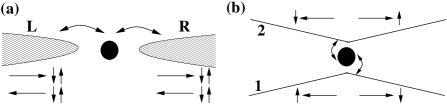
Figure 1: Setups considered in this Letter. (a) A quantum dot coupled to two 1d Luttinger leads $(L,R)$ where both left and right-moving electrons in the leads can be either in the spin up or spin down state. (b) A quantum dot coupled to (helical) edge states $(1,2)$ of topological insulators. The right and left moving electrons on the edges are spin polarized.

Equilibrium properties. Let us focus on the setup of Fig. 1(a). We denote by $g_{LR}$ and $g_{LL}=g_{RR}$ the dimensionless inter-lead and intra-lead Kondo couplings, respectively Glazman ; Lee . The RG analysis results in two infrared fixed points Gogolin ; Kim : the 1CK and 2CK fixed points. In the former case, all Kondo couplings, $g_{LR}$ and $g_{LL},$ are relevant under RG transformation and flows towards strong coupling, such that the two leads can be combined into a single effective lead. In contrast, the 2CK fixed point is reached when $g_{LR}$ remains small under RG, while $g_{LL}$ grows (and flow to intermediate coupling). Here, the two leads provide independent screening channels. This 2CK fixed point is infrared stable for $K<1/2$ (assuming that $g_{LL}=g_{RR}$) Gogolin ; Kim .

For $K=1$ (free electron leads), where 1CK physics is realized Glazman ; Lee , the conductance reaches the unitary limit at low temperatures, $G(T)=2G_{0}[1-\mathcal{O}((T/T_{\rm K})^{2})]$ where $G_{0}=e^{2}/h$ is the conductance quantum. Here, $T_{\rm K}\equiv D_{0}e^{-1/(g_{LR}^{0}+g_{LL}^{0})}$ is the Kondo temperature; $D_{0}$ is an ultraviolet cutoff $(\sim\hbox{few Kelvins})$ whereas $g_{LR}^{0}$ and $g_{LL}^{0}$ are the bare values of the coupling constants. For $T\gg T_{\rm K}$, from $G(T)\propto g_{LR}(T)^{2}$, one finds $G(T)\sim 1/\ln^{2}(T/T_{\rm K})$.

For all $K<1$, $g_{LR}$ grows slower under RG than $g_{LL(RR)}$. For $K\ll 1$, one can solve the RG equations analytically for large $T$. We may neglect $g_{LR}$ in the RG equation for $g_{LL/RR}$ to obtain the approximate solution $g_{LL/RR}(T)\approx 1/\ln(T/T_{K}^{*})$ with the shorthand $T_{K}^{*}\equiv D_{0}e^{-1/g_{LL}^{0}}$. The coupling $g_{LR}(T)$ is found by substituting the approximate solution for $g_{LL/RR}(T)$ in the RG equation for the coupling $g_{LR}$. We evaluate:

$$g_{LR}(T)\approx\frac{(T/D^{*})^{\frac{1}{2}(\frac{1}{K}-1)}}{\ln^{2}(T/T_{\rm K}^{*})}.$$ (1)

where $D^{*}=\frac{D_{0}}{[g_{LR}^{0}\ln^{2}(D_{0}/T_{\rm K}^{*})]^{s}}$ with $1/s=(1/K-1)/2$. We deduce that, for $T\gg T_{K}^{*}$, the conductance $G(T)\propto g_{LR}^{2}(T)$ essentially follows $T^{1/K-1}/\ln^{4}(T/T_{K}^{*})$. Here, the power-law behavior is reminiscent of Luttinger physics whereas the logarithmic contribution is typical of Kondo correlations. Importantly, the conductance is not a universal function of $(T/T_{K}^{*})$ because transport arises from the sub-leading coupling $g_{LR}$.

For $1/2<K<1$, the low-temperature physics is governed by two scales, $T_{\rm 1CK}<T_{\rm 2CK}$, with 1CK behavior for $T\ll T_{\rm 1CK}$ and 2CK behavior for $T_{\rm 1CK}\ll T\ll T_{\rm 2CK}$. In the limits $K\to 1$ and $K\to 0$, we have $T_{\rm 1CK}=T_{\rm K}$ and $T_{\rm 2CK}=T_{\rm K}^{*}$, respectively, with $T_{\rm K}$, $T_{\rm K}^{*}$ defined above. In general, $T_{\rm 1CK}\ll T_{\rm K}$ due to interactions in the leads; also, $T_{\rm 2CK}>T_{\rm K}^{*}$. In the presence of particle-hole symmetry, the conductance for $1/2<K<1$ reaches the unitary limit as $T\rightarrow 0$. However, potential scattering is a relevant perturbation with a scaling dimension $(1+K)/2<1$ and causes the conductance to decrease as $T^{1/K-1}$ as $T\rightarrow 0$; the leading irrelevant operator corresponds to the hopping ($g_{LR}$) term between the two leads with scaling dimension $(1/K+1)/2$. Similarly, near the 2CK fixed point reached for $K<1/2$ and $g_{LL}=g_{RR}$, the leading irrelevant operator ($g_{LR}$ term) has dimension $1/2K$ Kim , and therefore one expects $G(T)\propto T^{1/K-2}$ as $T\rightarrow 0$.

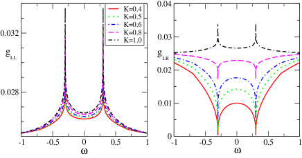
Figure 2: (Color online) $g_{LL}(\omega)$ and $g_{LR}(\omega)$ for various Luttinger parameters $K$. The bare couplings are $g_{\alpha\alpha^{\prime}}^{0}=g_{\alpha\alpha}^{0}=0.025$, resulting in $T_{K}^{*}\sim 4.2\times 10^{-18}$ and $T_{K}\sim 2\times 10^{-9}$ (in units of $D_{0}=1$). The bias voltage is $V=0.6\gg T_{K},T_{K}^{*}$.

Non-equilibrium properties. We study the low-temperature conductance in the high-bias regime $V\gg T_{\rm K},T_{\rm K}^{*}$ where the non-equilibrium RG method can be applied Rosch . (In the opposite limit, $V\ll T_{\rm K}^{*}$, we expect the equilibrium results quoted above to be valid after replacing $T\rightarrow V$.) Setting $\hbar=k_{B}=e=1$, the non-equilibrium RG equations take the form:

$$\frac{\partial g_{LL}(\omega)}{\partial\ln D} = -\sum_{\beta=-1,1}\left[g_{L\beta}\left(\frac{\beta V}{2}\right)\right]^{2}\Theta_{\omega+\frac{\beta V}{2}}$$

$$\frac{\partial g_{LR}(\omega)}{\partial\ln D} = -\sum_{\beta=-1,1}\frac{1}{4}\left[1-\frac{1}{K}\right]g_{LR}\left(\frac{\beta V}{2}\right)\Theta_{\omega+\frac{\beta V}{2}}$$ (2)

$$- g_{L\beta}\left(\frac{\beta V}{2}\right)g_{\beta R}\left(\frac{\beta V}{2}\right)\Theta_{\omega+\frac{\beta V}{2}},$$

where $\Theta_{\omega}=\Theta(D-|\omega+\mathit{i}\Gamma|)$ and $\beta=-1(+1)$ labels leads $L(R)$. Further, $\Gamma$ is the decoherence (dephasing) rate at finite bias which cuts off the RG flow Rosch :

$$\Gamma=\pi\sum_{\alpha\alpha^{\prime}}\int{d\omega f_{\omega}^{\alpha}\left(1-f_{\omega}^{\alpha^{\prime}}\right)[g_{\alpha\alpha^{\prime}}(\omega)]^{2}},$$ (3)

where the Fermi function obeys $f^{\alpha}(\omega)=1/(1+e^{(\omega-\mu_{\alpha})/T})$. We note that there exists an additional contribution to $\Gamma$ from electron dephasing caused by a finite potential drop in the Luttinger liquid leads Mirlin , which will affect the subleading terms in $\Gamma$ (given by $g_{LR}(V/2)$). However, in the low-conductance regime of interest, this voltage drop is small and will be neglected henceforth. In general, the perturbative RG approach is valid for $V\gg T_{\rm 1CK},T_{\rm 2CK}$. In the limit of $V\rightarrow 0$, Eqs. (2) reduce to the equilibrium RG equations (with the flow cut off by temperature), and we recover Eq. (1).

The renormalized couplings are obtained by self-consistently solving Eqs. (2) and (3) Rosch . As shown in Fig. 2, $g_{LL(RR)}(\omega)$ exhibit peaks for all values of $K\leq 1$, indicating that they grow under RG. For a given bias voltage, the Kondo coupling $g_{LR}(\omega)$ shows a crossover from peak to dip structure as $K$ decreases, traducing the fact that for a fixed bias voltage, $g_{LR}(\omega)$ is either enhanced or decreased compared to its bare value $g_{LR}^{0}$. Let us emphasize that for sufficiently large bias voltages, as soon as $K<1$ the coupling $g_{LR}(\omega)$ exhibits a dip close to $\omega=\pm V/2$, signalling 2CK behavior. The singular behavior at the peaks or dips is cut off by the decoherence rate (see Eq. (6)), while outside that regime the voltage serves to cut off the RG flow.

From the Keldysh calculation up to second order in the tunneling amplitudes, the current reads:

$$I=\frac{3\pi}{4}\int d\omega\Big{[}\sum_{\sigma}g_{LR}(\omega)^{2}f_{\omega}^{L}(1-f_{\omega}^{R})\Big{]}-(L\leftrightarrow R).$$ (4)

For small bare couplings $g_{\alpha\alpha^{\prime}}^{0}=g_{\alpha\alpha}^{0}$ this perturbative calculation of $I$ remains valid for $V>T_{\rm K}^{*}$, implying at high bias voltage $V\gg T$ contributions to the current over a frequency window $-V/2<\omega<V/2$. For bias voltages $T_{\rm K}^{*}<V\ll D_{0}$, with decreasing $V$ we find the differential conductance $G(V)\equiv dI/dV$ approaches the equilibrium form of the conductance $G(T\rightarrow V)\propto V^{1/K-1}/\ln^{4}(V/T_{\rm K}^{*})$ with $G(T)\propto g_{LR}(T)^{2}$ (see Eq. (1) and Fig. 3).

In the remainder, we analyze $G(V)$ for larger bias voltages. For $K=1$, we checked that the nonlinear conductance satisfies $G(V)\propto 1/\ln^{2}(V/T_{\rm K})$ for $V\gg T_{\rm K}$ Kaminski . Here, one can replace $g_{LR}(\omega)$ by $g_{LR}(\omega=0)\approx g_{LR}(T\rightarrow V)$. When decreasing $K$, the double peak structure in $g_{LR}(\omega)$ at $\omega=\pm V/2$ turns progressively into dips which acquire a complex shape as a result of the decoherence rate $\Gamma$ and the electron-electron interaction which hinders the inter-lead electron tunneling. The effect becomes more pronounced for small $K$ values associated with the 2CK fixed point, rendering the “flat” approximation $g_{LR}(\omega)\approx g_{LR}(\omega=0)$ not justified; see Fig. 3.

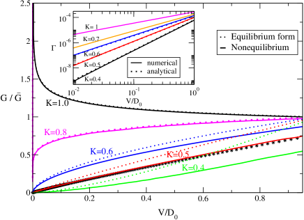
Figure 3: (Color online) $G(V)$ normalized to $\bar{G}=3\pi(g_{LR}^{0})^{2}/4$ for various $K$ and Kondo couplings as in Fig. 2. Here, “Equilibrium form” refers to a fit with the expression $G(V)=3\pi g_{LR}(\omega=0)^{2}/4$ which consists in substituting $g_{LR}(\omega)$ by $g_{LR}(\omega=0)$ for $|\omega|<V/2$. For $K=0.5$ we also show the analytical result from Eqs. (7,8) (stars). Inset: $\Gamma(\omega=0,V)$ for various $K$. The dashed lines are obtained from the analytical expression in Eq. (9). Here, $D_{0}=1$.

To gain an analytical understanding of the small-$K$ non-equilibrium regime, we may treat $g_{RL}(\omega)$ within the interval $-V/2<\omega<V/2$ as a semi-ellipse chung . The current $I$ reads

$$I\approx\frac{3\pi}{4}\left[\frac{\pi}{4}g_{LR}(\omega=0)^{2}+\left(1-\frac{\pi}{4}\right)g_{LR}(\omega=V/2)^{2}\right].$$ (5)

For $K<1$, we manage to obtain an approximate analytical form for the couplings $g_{LR}(\omega=V/2)$ and $g_{LR}(\omega=0)$. Solving Eqs. (2) in the limit $D\rightarrow 0$, we find:

$$g_{LR}(\omega=0) \approx g_{LR}(T\rightarrow V){\cal F}(K)$$ (6)

$$g_{LR}\left(\frac{V}{2}\right) \approx \frac{4\left(\frac{\Gamma V}{D^{*2}}\right)^{\frac{1}{4}(\frac{1}{K}-1)}}{\ln^{2}\left(\frac{\Gamma V}{(T_{\rm K}^{*})^{2}}\right)},$$

where $g_{LR}(T\rightarrow V)$ is the equilibrium form of $g_{LR}$ in Eq. (1) with $T$ replaced by $V$, and we have defined ${\cal F}(K)=2^{1+\frac{1}{4}(1-1/K)}-1$, with ${\cal F}(K=1)=1$. Using Eqs. (5) and (6), we obtain a closed expression for the conductance:

$$G(V) \approx \frac{3\pi^{2}}{16}\left(\frac{V}{D^{*}}\right)^{\frac{1}{K}-1}{\cal R}(V)$$

$$+ 12\pi\left(1-\frac{\pi}{4}\right){\cal W}^{\prime}(V),$$

where ${\cal W}^{\prime}(V)=d{\cal W}/dV$ and:

$${\cal R}(V) = {\cal F}(K)^{2}\left[\frac{1/K}{\ln^{4}\left(\frac{V}{T_{\rm K}^{*}}\right)}-\frac{4}{\ln^{5}\left(\frac{V}{T_{\rm K}^{*}}\right)}\right]$$ (8)

$${\cal W}(V) = \frac{V(\Gamma V/D^{*2})^{\frac{1}{2}(\frac{1}{K}-1)}}{\ln^{4}[\Gamma V/(T_{\rm K}^{*})^{2}]}.$$

For completeness, we have kept the less dominant contribution $\sim 1/\ln^{5}(V/T_{\rm K}^{*})$ in ${\cal R}(V)$. To rigorously define the function ${\cal W}(V)$, we need to provide an analytical expression for the decoherence rate in Eq. (3).

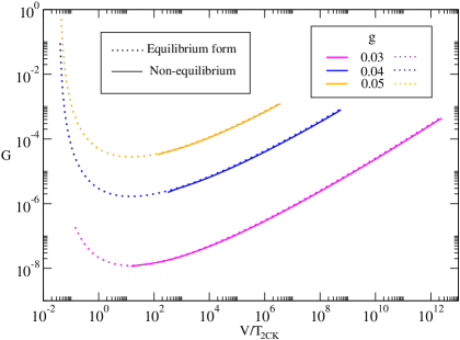
Figure 4: (Color online) $G$ versus $V/T_{\rm 2CK}$ for $K=0.6$ for various initial Kondo couplings $g_{\alpha\alpha^{\prime}}^{0}=g_{\alpha\alpha}^{0}=g$ (in units of $D_{0}=1$).

Using an analogous reasoning as for the non-equilibrium current $I$, to second order in $g_{LR}^{0}$, we extract

$$\Gamma\approx\frac{\pi^{2}}{4}{\cal F}(K)^{2}\frac{V\left(\frac{V}{D^{*}}\right)^{\frac{1}{K}-1}}{\ln^{4}\left(\frac{V}{T_{K}^{*}}\right)}.$$ (9)

Close to $K=1/2$, we can safely neglect contributions in $(g_{LR}^{0})^{2+(1/K-1)}$ and therefore to second order in $g_{LR}^{0}$, we find $\Gamma\approx(\pi^{2}/4)[g_{LR}(\omega=0)]^{2}$. We have checked our analytical expression of $\Gamma$ against a numerical treatment of Eqs. (2) and (3); see inset in Fig. 3. Notably, the decoherence rate contributes to a “distinct” power law $\sim V^{\frac{1}{2}\left(\frac{1}{K^{2}}-1\right)}$ in the non-equilibrium conductance $G(V)$ where $(1/K^{2}-1)/2>1/K-1$ for $K<1$, rendering the second term in Eq. (7) to be subleading. The conductance becomes smaller than its equilibrium counterpart since $g_{LR}(\omega=V/2)<g_{LR}(\omega=0)$. A comparison between the analytical formula in Eq. (7) and the numerical integration of Eqs. (2-4) is shown in Fig. 3. As our results are based on one-loop RG, we may expect both corrections to the power-law prefactors and further subleading terms upon including higher-loop contributions.

Our results show that $G(V)$ for voltages $T_{\rm 2CK}\ll V\ll D_{0}$ is not an universal function of $V/T_{\rm 2CK}$ (even for fixed $K$): Fig. 4 displays $G$ versus $V/T_{\rm 2CK}$ for various initial Kondo couplings, with $T_{\rm 2CK}$ extracted from the RG flow. As it becomes also clear from Eqs. (7,8), the non-equilibrium conductance for $V\gg T_{\rm 2CK}$ is a function of both $V/D_{0}$ and $V/T_{\rm K}^{*}$, and hence has a non-universal profile. This is again related to the fact that transport arises from the subleading coupling $g_{LR}$.

Topological insulators. We can extend these results to a quantum dot coupled to helical edges of 2d TIs; see Fig. 1(b). In contrast with the setup of Fig. 1(a) where single-particle backscattering terms caused by the quantum dot cut the system into two separate parts, such backscattering terms are now forbidden due to time-reversal symmetry of the helical edges Wu ; PLee . Following Refs. Hou, ; Teo, , the two edges of spinless electrons can be mapped onto spinful Luttinger liquids with distinct Luttinger parameters for charge ($K_{c}$) and spin ($K_{s}$) degrees of freedom: $K_{c}=\bar{K}$, and $K_{s}=1/\bar{K}$ with $\bar{K}$ being Luttinger parameter for the helical edges. In equilibrium, the system is equivalent to an anisotropic 2CK model with the Kondo couplings $g_{\alpha\beta}^{xy,z}$ ($\alpha,\beta=1,2$) PLee and in contrast to the case in Fig. 1(a), the 2CK fixed point is stable for $\bar{K}<1$. In the limit of $\bar{K}\to 1^{-}$ where the anisotropy in the Kondo couplings is negligible, we have checked that the RG scaling equations for the Kondo couplings $g_{11/22}$ and $g_{12}$ are identical to those of the Kondo couplings $g_{LL/RR}$ and $g_{LR}$. We identify: $g_{LL/RR}\to g_{11/22}$, $g_{LR}\to g_{12}$, $\frac{1}{K}\to\bar{K}+1/\bar{K}-1$ RGTI . Our results on non-equilibrium transport across a quantum dot coupled to weakly interacting Luttinger leads are directly applicable.

Summary. We have studied non-equilibrium transport through a Kondo dot coupled to Luttinger-liquid leads and calculated the conductance profile at bias voltages larger than the Kondo scales of the system. The RG flow at large bias shows signatures of intermediate 2CK physics for all Luttinger parameters $K<1$. As the conductance $G$ arises from the coupling $g_{LR}$ which is subleading, $G(T\to 0)$ is not a universal function of $V/T_{\rm 2CK}$ as it also depends on $V/D_{0}$. Our results push forward the knowledge of correlation effects in nanosystems far from equilibrium and should stimulate further experimental works on transport through dots coupled to quantum wires and carbon nanotubes. We have also shown that our theoretical framework is applicable to the Kondo effect at the helical edges of topological insulators.

We thank A. Rosch for many helpful discussions. This work is supported by the NSC grant No.98-2918-I-009-06, No.98-2112-M-009-010-MY3, the MOE-ATU program, the NCTS of Taiwan, R.O.C. (C.H.C.), the Department of Energy in USA under the grant DE-FG02-08ER46541 (K.L.H.), and the DFG via SFB 608, SFB/TR-12 (M.V.), and the Center for Functional Nanostructures (P.W.). KLH thanks the kind hospitality of LPS Orsay.

References

- (1) R. M. Potok et al., Nature 447 167-171 (2007).
- (2) A. Rosch et al., Phys. Rev. Lett. 90, 076804 (2003) and J. Phys. Soc. Jpn. 74, 118 (2005).
- (3) S. Kehrein, Phys. Rev. Lett. 95, 056602 (2005).
- (4) P. Mehta and N. Andrei, Phys. Rev. Lett. 96, 216802 (2006).
- (5) E. Boulat, H. Saleur, and P. Schmitteckert, Phys. Rev. Lett. 101, 140601 (2008).
- (6) F. B. Anders, Phys. Rev. Lett. 101, 066804 (2008).
- (7) C. Mora et al., Phys. Rev. B 80, 155322 (2009).
- (8) L. I. Glazman and M. E. Raikh, JETP Lett. 47, 452 (1985).
- (9) T. K. Ng and P. A. Lee, Phys. Rev. Lett. 61, 1768 (1988).
- (10) K. Le Hur, Phys. Rev. Lett. 92, 196804 (2004); M.-R. Li, K. Le Hur, and W. Hofstetter, Phys. Rev. Lett. 95, 086406 (2005).
- (11) K. Le Hur and M.-R. Li, Phys. Rev. B 72, 073305 (2005).
- (12) S. Florens et al., Phys. Rev. B 75, 155321 (2007).
- (13) A. Furusaki and K. A. Matveev, Phys. Rev. Lett. 88, 226404 (2002).
- (14) M. Fabrizio and A. O. Gogolin, Phys. Rev. B 51, 17827 (1995).
- (15) E. Kim, cond-mat/0106575 (unpublished).
- (16) H. Steinberg et al., Nature Physics 4, 116 (2008).
- (17) Y.-W. Lee and Y.-L. Lee, Phys. Rev. B 65, 155324 (2002).
- (18) Y.-L. Liu and T. K. Ng, Phys. Rev. B 61, 2911 (2000).
- (19) C.-H. Chung et al., Phys. Rev. Lett. 102, 2106803 (2009).
- (20) D. B. Gutman, Y. Gefen and A. D. Mirlin, arXiv:0906.4076 and arXiv:0911.4559.
- (21) Y. F. Chen et al., Phys. Rev. Lett. 102, 036804 (2009).
- (22) C. Wu, B. A. Bernevig, and S.-C. Zhang, Phys. Rev. Lett. 96, 106401 (2006).
- (23) J. Maciejko et al., Phys. Rev. Lett. 102, 256803 (2009).
- (24) K. T. Law et al., arXiv:0904.2262.
- (25) A. Kaminski, Yu. V. Nazarov and L. I. Glazman, Phys. Rev. Lett. 83, 384 (1999).
- (26) C.-Y. Hou, E.-A. Kim and C. Chamon, Phys. Rev. Lett. 102, 076602 (2009).
- (27) C. Y. Teo and C. L. Kane, Phys. Rev. B 79, 235321 (2009).
- (28) The scaling dimensions of the couplings are , , .