The ACS Nearby Galaxy Survey Treasury V. Radial Star Formation History of NGC 300

Abstract

We present new Hubble Space Telescope (HST) observations of NGC 300 taken as part of the ACS Nearby Galaxy Survey Treasury (ANGST). Individual stars are resolved in these images down to an absolute magnitude of $M_{F814W}=1.0$ (below the red clump). We determine the star formation history of the galaxy in 6 radial bins by comparing our observed color-magnitude diagrams (CMDs) with synthetic CMDs based on theoretical isochrones. We find that the stellar disk out to 5.4 kpc is primarily old, in contrast with the outwardly similar galaxy M33. We determine the scale length as a function of age and find evidence for inside-out growth of the stellar disk: the scale length has increased from $1.1\pm 0.1$ kpc 10 Gyr ago to $1.3\pm 0.1$ kpc at present, indicating a buildup in the fraction of young stars at larger radii. As the scale length of M33 has recently been shown to have increased much more dramatically with time, our results demonstrate that two galaxies with similar sizes and morphologies can have very different histories. With an $N$-body simulation of a galaxy designed to be similar to NGC 300, we determine that the effects of radial migration should be minimal. We trace the metallicity gradient as a function of time and find a present day metallicity gradient consistent with that seen in previous studies. Consistent results are obtained from archival images covering the same radial extent but differing in placement and filter combination.

1. Introduction

The standard model of galaxy formation has the inner parts of galaxies forming before the outer parts, as a result of increasing timescales for gas infall with radius (Larson, 1976; White & Frenk, 1991; Burkert et al., 1992; Mo et al., 1998; Naab & Ostriker, 2006). This “inside-out” growth scenario has likewise been seen in $N$-body/Smooth Particle Hydrodynamics simulations of disk galaxy evolution (Brook et al., 2006), and has been used to explain the observed abundance gradients in the Milky Way via chemical evolution models (Matteucci & Francois, 1989; Chiappini et al., 1997; Boissier & Prantzos, 1999).

There are multiple mechanisms which could contribute to an observed trend of star formation taking place more recently in the outer parts of galaxies. The first, as previously mentioned, is that gas does not accumulate in the outer disk until later times, or that it accumulates more slowly such that the total mass density of the outer disk increases with time. Alternatively, if the gas is in place but the star formation timescale in the outer disk is longer, the stellar mass density would increase more slowly with time in the outer disk.

If disks do form “inside-out,” one would expect to see negative radial gradients in age and metallicity. Age gradients would result from a higher percentage of older stars in the centers of galaxies, where star formation started earlier. This older population of stars would enrich the surrounding gas, causing more recently formed stars toward the center to be more metal-rich than stars formed in the outskirts of the disk.

Negative gradients have been seen in several surveys of nearby galaxies, and they appear to be common, if not universal, among larger disks. In the sample of nearby galaxies presented in Muñoz-Mateos et al. (2007), $\mathrm{FUV}-K$ color was used as a proxy for star formation rate (SFR), since it represents the ratio of young to old stars and shows what fraction of the total star formation has been recent. Large spirals were found to have predominantly negative gradients, while low-luminosity systems show a considerable scatter in the slopes of their gradients, with both positive and negative values, indicating a wider range of possible formation histories. The MacArthur et al. (2009) study of nearby spirals using spectral synthesis finds both negative gradients and flat profiles in stellar age and metallicity.

A flat radial profile in age and metallicity may be consistent with inside-out growth if gradients established early were erased by interactions or subsequent radial migration. Especially in high-mass systems, stars can scatter off of spiral structure and change their radii while retaining circular orbits (Sellwood & Binney, 2002). The simulations of Roškar et al. (2008) showed that some percentage of older stars currently residing in the outer disk of a galaxy actually formed closer to the center of the disk and migrated outward to their current location. Thus, an observed older stellar population in the outer disk of a massive galaxy may not necessarily indicate that the outer disk formed early.

The ideal galaxies for studying the evolution of disks in the absence of major mergers are undisturbed, pure-disk (i.e., bulgeless) systems that maintain weak spiral structure to suppress radial migration. While one method of studying galaxy evolution is to compare high-redshift galaxies with their local counterparts, difficulties with this method include the dramatic falloff of surface brightness with redshift and the inability to trace the history of a single galaxy. Color-magnitude diagrams (CMDs) derived from resolved stellar populations can provide detailed, time-resolved studies of the disk evolution. This method restricts the possible targets to relatively local galaxies.

NGC 300, in the Sculptor Group, is the nearest isolated late-type disk galaxy, and is thus an ideal target. Muñoz-Mateos et al. (2007) have already suggested an inside-out growth scenario for NGC 300 based on its broadband colors. The resolution of the Hubble Space Telescope (HST) enables us to use CMD fitting to find the star formation histories (SFHs) of galaxies outside the Local Group. The ACS Nearby Galaxy Survey Treasury (ANGST; Dalcanton et al., 2009) was designed to create a volume-limited sample of nearby galaxies, allowing for an unbiased accounting of star formation in the nearby universe. The continuous radial strip of NGC 300 imaged as part of ANGST allows us to recover the SFH of this galaxy out to $\sim 5$ kpc.

Table 1 Summary of NGC 300 and M33 properties

	NGC 300	M33
Distance	2.0 Mpc	800 kpc
Type	SA(s)d	SA(s)cd
$M_{B}$	-17.66	-18.4
Scale length ($K$)	1.3	1.4
Circular velocity	97 km s-1	130 km s-1
Estimated mass	$2.4\times 10^{10}$ $M_{\sun}$	$5\times 10^{10}$ $M_{\sun}$

Evidence for inside-out growth (a decrease in mean stellar age with radius) has also been found in M33, a galaxy very similar to NGC 300 (see Table 1 for a comparison of their main properties). In M33, Williams et al. (2009a) and Holtzman et al. (in prep.) used resolved stellar populations from four HST/ACS fields to derive SFHs using CMD fitting. From these SFHs, they infer the stellar surface density of the disk at different times throughout the galaxy’s history and find significant evolution in the scale length of the disk. The increase in scale length with time, indicating that the SFR has been increasing in the outer disk, is suggestive of inside-out growth.

While outwardly similar, NGC 300 and M33 may have different histories. M33 has a disk break at $\sim 6$ scale lengths (Ferguson et al., 2007), which is a common feature in spiral galaxies (Pohlen & Trujillo, 2006). However, Bland-Hawthorn et al. (2005) showed that NGC 300 has a pure exponential disk out to $\sim 10$ scale lengths. There are environmental differences as well: an Hi bridge between M33 and M31 is suggestive of a history of interaction between these two galaxies (Braun & Thilker, 2004; Bekki, 2008), a finding that is confirmed by the distribution of red giant branch (RGB) stars surrounding the two galaxies (McConnachie et al., 2009) and the evidence for tidal disruption of M33’s gas disk (Putman et al., 2009). In contrast, NGC 300 is fairly isolated on the Sculptor filament, with only dwarf galaxies nearby (Karachentsev et al., 2003). These differences may imply significantly different SFHs.

In §2, we describe our data and reduction; in §3, we describe our methods for determining the star formation history and present our results; we discuss their implications for disk growth along with possible caveats and compare our metallicity results to other observations in §4, and we conclude with §5. Archival data is presented in Appendix A. We adopt a WMAP cosmology (Spergel et al., 2007) for all conversions between time and redshift.

2. Data and Photometry

2.1. ACS Imaging

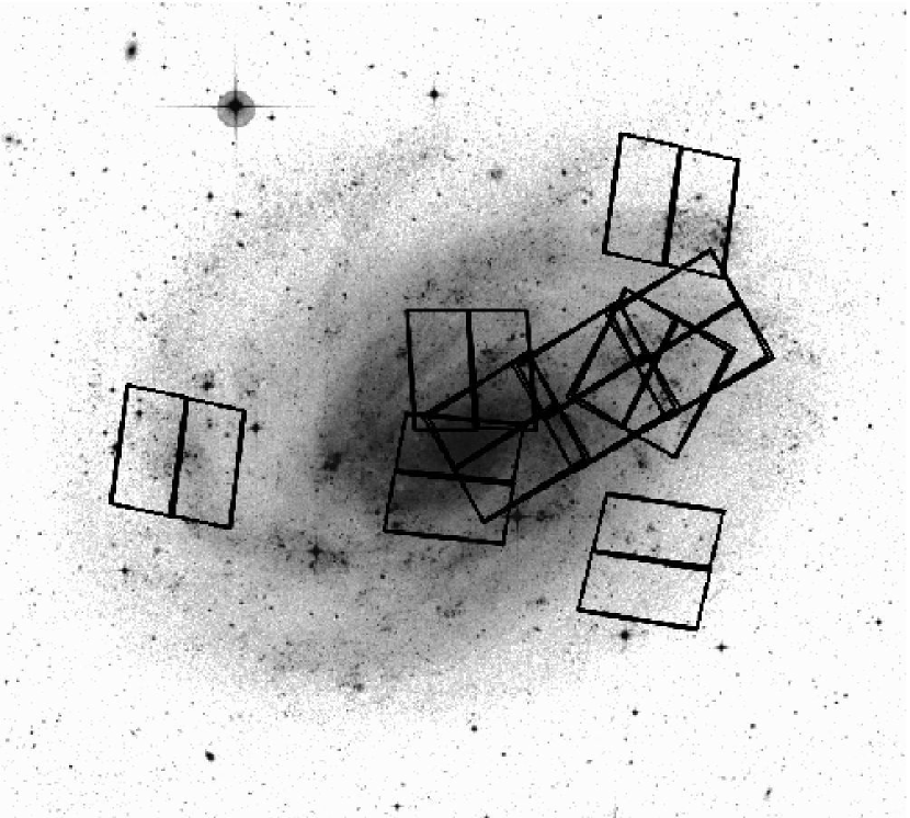
Figure 1.— DSS image of NGC 300 with ACS fields overlaid. The three contiguous ACS fields forming a radial strip are from ANGST, while the other fields are archival data.

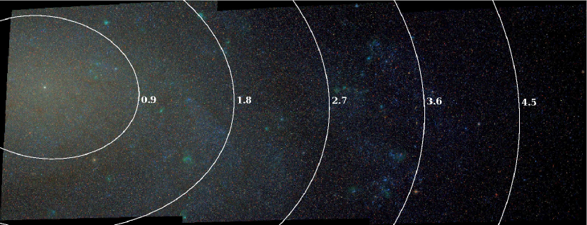
Figure 2.— Color image of the radial strip of NGC 300 observed as part of ANGST (red: $F814W$, green: $F606W$, blue: $F475W$). Inclination-corrected radial bins of width 0.9 kpc are overlaid as white lines, with radii in kpc labeled.

As part of ANGST (GO-10915), we took HST Advanced Camera for Surveys (ACS; Ford et al., 1998) observations of NGC 300 during 2006 November 8-10. Three slightly overlapping fields were observed along a radial strip from the center of the galaxy into the disk. Each field was observed for 1488s in $F475W$, 1515s in $F606W$, and 1542s in $F814W$. An additional deep outer field was planned as part of the ANGST program, which would have given more extended radial coverage of the disk; unfortunately, ACS failed before this observation was obtained.

An additional six archival ACS images, scattered across the disk of NGC 300, are presented in Appendix A. We include the archival data as a useful consistency check that the ANGST data is representative of the disk as a whole. However, since the observing conditions were not identical (different exposure times, different filters, and no spatial continuity), we keep the analysis of the archival data separate from that of the new observations. These images were originally taken as part of the Araucaria project to determine Cepheid distances to nearby galaxies (GO-9492), so the fields were selected to sample the Cepheid population at different galactocentric distances and are therefore placed on more active star-forming regions (Bresolin et al., 2005; Rizzi et al., 2006). The observations were obtained between the dates of 2002 July 17 and December 25, with exposure times of 1080s in $F435W$ and $F555W$, and 1440s in $F814W$. Each observation was split between two exposures for cosmic-ray removal and coverage of the chip gap. The exposures were calibrated and flat-fielded using the standard HST pipeline. The locations of all ACS fields are shown in Figure 1.

2.2. Photometry

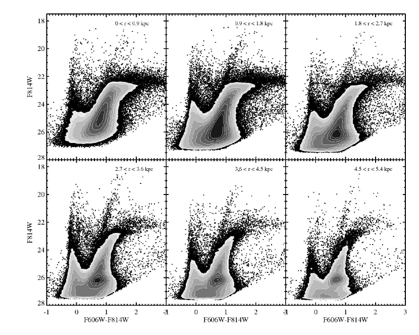
Figure 3.— CMDs of radial bins from ANGST data. Only stars with S/N $>4$ and high-quality photometry have been included (see §2.2).

While exposures were combined using MultiDrizzle to produce images in this paper, photometry was done using all individual exposures simultaneously. For photometry, we use DOLPHOT, a modified version of HSTphot (Dolphin, 2000) optimized for the ACS. DOLPHOT fits the ACS point spread function (PSF) to all of the stars in each exposure, determines the aperture correction from the most isolated stars, combines the results from all exposures, and converts the count rates to the Vega magnitude system. Details of the photometry and quality cuts used for the ANGST sample and archival data are given in Williams et al. (2009b) and Dalcanton et al. (2009). We require that stars in the final sample are classified as stars, not flagged as unusable (too many bad or saturated pixels or extending too far off the edge of the chip), have $S/N>4$, and have $|sharp_{F606W}+sharp_{F814W}|<0.274$. Sharpness indicates whether a star is too sharp (perhaps a cosmic ray) or too broad, and these cuts exclude non-stellar objects (such as background galaxies) that escaped the earlier cuts. We also cut on the crowding parameter, which is defined as how much brighter a star would have been measured if nearby stars had not been fit simultaneously. Stars with a high crowding parameter are more likely to have erroneous photometry, but a very strict cut has the effect of preferentially removing young stars, since these are usually found in clusters. We require $crowd_{F606W}+crowd_{F814W}<0.6$ mag.

We characterize the completeness of our sample in terms of magnitude, color, and position by inserting at least $\sim 10^{6}$ artificial stars ($\sim 50,000$ stars at a time) in each ACS field. DOLPHOT is also used to perform the artificial star tests. Individual stars are inserted into the original images and their photometry is re-measured. Artificial stars are labeled as “detected” if they were found by DOLPHOT and met the quality cuts described above. The 50% completeness limit for ANGST ranges from $F606W=26.7,F814W=25.8$ in the crowded center of the galaxy to $F606W=28.4,F814W=27.4$ in the outer regions. For the archival data, 50% completeness limits range from $F555W=26.8$ to 27.7 and $F814W=25.8$ to 27.2.

2.3. Identification of Duplicate Stars

The ANGST fields overlap by $\sim 7\arcsec$ so that the fields could be aligned into a single radial strip. When combining the photometry of all stars into a single catalog, we identify and remove duplicate stars in overlapping regions by binning star positions in each field and finding bins that contain stars from more than one field. The bin size is set at $1\arcsec$, big enough so that nearly all bins in the overlap regions contain stars in both fields but small enough so that the edges of the overlap regions are fairly smooth. The three ANGST fields are designated WIDE1, WIDE2, and WIDE3, with WIDE3 containing the center of the galaxy and WIDE1 farthest from the center. For the WIDE1-WIDE2 overlap, stars in WIDE1 are kept, and for the WIDE2-WIDE3 overlap, stars in WIDE2 are kept. The World Coordinate System (WCS) for each of 3 fields is provided by the standard HST pipeline, but there are very small offsets between fields. We found that relative to WIDE2, WIDE1 has an offset of $\Delta\alpha=0.23\arcsec,\Delta\delta=0.036\arcsec$, and WIDE3 has an offset of $\Delta\alpha=-0.13\arcsec,\Delta\delta=-0.14\arcsec$.

2.4. Dividing Stars into Radial Bins

To assign an inclination-corrected galactocentric distance to each star, we assume the following galaxy parameters: $\alpha_{0}=13.722833\arcdeg$, $\delta_{0}=-37.684389\arcdeg$ (galaxy center), $i=42\arcdeg$ (inclination), $\theta=111\arcdeg$ (position angle) (Kim et al., 2004). To convert radius on the sky to physical distance, we assume a distance of 2.0 Mpc to NGC 300, which is the distance we measure using the tip of the red giant branch (TRGB) (Dalcanton et al., 2009). The maximum radius we find for a star in the ANGST fields is $r=5.35$ kpc.

Stars are divided into 6 radial bins based on their (inclination-corrected) distance from the center of the galaxy. Artificial stars are divided in the same way. Our bins are spaced 0.9 kpc apart in radius, to encompass all of the observed stars in annuli of equal width (Figure 2). The spacing of the bins is motivated by the length over which we expect radial mixing to blur the populations (Roškar et al., 2008). The observed area is calculated for each bin so that we can derive the correct surface density of star formation. CMDs for stars in each bin are shown for the ANGST data in Figure 3.

In the various fits to distance shown in §4 and Appendix A, the distance used for each radial bin is the mean distance from the center of pixels in that region.

3. Star Formation History Analysis

3.1. Method

Figure 4.— Lifetime SFHs of radial bins from ANGST data. Error bars are the quadrature sum of the uncertainties from distance and extinction and the 68% confidence interval from Monte Carlo simulations. SFRs have been scaled to a Kroupa (2002) IMF. The scale of the vertical axis differs in each panel.

To derive the SFH of each radial bin, we use the well-established technique of comparing the observed CMD to a set of model CMDs (e.g., Gallart et al., 1999; Hernandez et al., 1999; Holtzman et al., 1999; Dolphin, 2002; Skillman et al., 2003; Harris & Zaritsky, 2004; Gallart et al., 2005). Typical fitting codes use stellar evolution models that predict the properties of stars of different masses for a range of ages and metallicities. From the predicted luminosity and temperature, the magnitudes of the stars are determined for a given filter set. Stars are then placed on a synthetic CMD following the mass distribution of an assumed initial mass function (IMF) and binary fraction for each age and metallicity. With distance and extinction either set or included as additional free parameters, these model CMDs are linearly combined until the best fit to the observed CMD is found. The ages and metallicities of the CMDs that went into the best fit tell us the ages and metallicities of the underlying stellar population, while the weights given to the CMDs provide the SFR at each age.

We use MATCH, described in Dolphin (2002), to derive the SFH for each radial bin. This code finds the maximum-likelihood fit to the CMD assuming Poisson-sampled data. We assume an IMF with a slope of -2.35 (Salpeter, 1955) between 0.1 and 120 $M_{\sun}$ and a binary fraction of 0.35. Given that our CMD only includes stars with masses $>1$ $M_{\sun}$, adopting a single Salpeter slope is likely to be a valid assumption. While a power-law IMF was used by MATCH for computational ease, the SFRs we show have been scaled to a Kroupa (2001) IMF. This is possible because, for stars massive enough to be observed, the two IMFs are very similar. The choice of IMF affects only the normalization of the SFH, but not the time dependence, so relative differences among age and radial bins do not depend on the IMF.

Synthetic CMDs are constructed from the theoretical isochrones of Girardi et al. (2002) and Marigo et al. (2008) for ages in the range 4 Myr–14 Gyr. The isochrones younger than $\sim 6\times 10^{7}$ yr were adopted from Bertelli et al. (1994), with transformations to the ACS system from Girardi et al. (2008). Age bins are spaced logarithmically, since the CMD changes much more rapidly at young ages than at old ages. Metallicity is allowed to vary in the range $-2.3<\rm{[M/H]}<0.1$, but is not allowed to decrease with time. See §4.3 for a further discussion of metallicity and uncertainties therein.

MATCH determines the best fit for distance and extinction by testing a range of values. The range for the distance modulus is $26.3\leq m-M\leq 26.7$, spanning the range of values reported in the literature (e.g., Butler et al., 2004; Sakai et al., 2004; Gieren et al., 2005; Rizzi et al., 2006; Dalcanton et al., 2009) and the extinction range is $0.05\leq A_{V}\leq 0.5$. Additionally, up to 0.5 mag of differential extinction is applied to young stars ($<100$ Myr), since these stars are more likely to be found in dusty star formation regions (Zaritsky, 1999; Zaritsky et al., 2002). The Schlegel et al. (1998) value for Galactic extinction is $A_{V}=0.042$ in the line of sight to NGC 300, but we expect the total value to be higher due to local extinction within NGC 300 itself. Additionally, we expect that dust content may vary across the extent of the disk, so extinction may be different in each radial bin.

Completeness and observational errors are accounted for by including the results of artificial star tests. We identify the artificial stars that were placed within each radial bin and supply MATCH with their input and output magnitudes and whether they were detected above the quality cuts of our photometry. The density distribution of artificial stars mirrors the density of detected stars within each bin, so MATCH accounts for any radial variation in crowding.

We use the $V+I$ equivalent filter sets ($F606W+F814W$, $F555W+F814W$) to derive the SFHs in this paper, due to the greater depth of the $F606W$ and $F555W$ data as compared to the $F457W$ and $F435W$ data. As a consistency check, we also derived the SFHs using $F475W+F814W$ for the ANGST fields and found SFHs that were consistent within the error bars (which are larger in $F475W+F814W$, especially in the inner regions), so our color choice does not appear to affect our conclusions significantly.

We assess uncertainties due to Poisson sampling of underpopulated regions in the CMD by running Monte Carlo simulations as follows: for each region, we sample stars at random from the observed CMDs until we reach the same number of stars as observed. These stars are then given as the input to MATCH with the distance and extinction fixed, and the resulting SFH is compared to the SFH from the original data. We repeat this process 100 times and define our sampling error as the values which encompass 68% ($1\sigma$) of the Monte Carlo tests. Our final error bars are the quadrature sum of this error and the systematic errors from fitting the distance and extinction. Our error bars do not include systematic uncertainties in the stellar evolution models.

3.2. Distance, Extinction, and Crowding Effects

Figure 5.— Recent ($<1$ Gyr) SFHs of radial bins from ANGST data. Errors are calculated as in Figure 4. SFRs have been scaled to a Kroupa (2002) IMF. The scale of the vertical axis differs in each panel. The bin at $2.7<r<3.6$ kpc contains a prominent spiral arm.

Because our data span a large range of stellar densities, the effective completeness varies strongly with radius. To deal with this variation, we pursued two independent methods. The first approach is to consider only the portion of the CMD that is 50% complete for each radial bin, so that larger portions of the CMD can be used in the outer, less crowded regions. The second approach is to find the completeness in the most crowded region (the center of the galaxy) and apply that magnitude cut to every region uniformly. This removes useful data in the outer regions, but ensures that variations we see in the SFH across the disk are not due to variations in photometric depth. We have employed both methods and compared the results.

When we allow the completeness cut to vary with radius, the photometry in the outer four radial bins is complete to well below the red clump (see Figure 3). This depth allows for a more consistent distance measurement across these four fields; derived distance modulus values for the ANGST data in the six radial bins were as follows: $m-M=26.61\pm 0.07,26.60\pm 0.07,26.43\pm 0.09,26.43\pm 0.09,26.42\pm 0.09,26.43\pm 0.09$. All of the four outer bins, with depths that resolve the red clump, produce a consistent estimate for the distance of $m-M=26.43\pm 0.09$. The inner fields, where crowding limits the depth, have a discrepant distance. We hereafter fix the distance to $m-M=26.43$ in all fields. Even if this distance is not absolutely correct, what is important is that setting the distance to the same value for all fields ensures that any relative changes in the positions of stars on the CMDs between radial bins are interpreted as differences in SFR and/or extinction.

Comparing the SFH when depth is allowed to increase with radius and the SFH where depth is at a fixed magnitude throughout, the recent SFHs for ages $<1$ Gyr are very similar, probably because the recent SFH is constrained by younger, brighter stars and is not significantly affected by the elimination of stars near the bottom of the CMD. For ages $>1$ Gyr, the most significant difference is a 40–80% increase in the SFR at 8–14 Gyr for the outer 3 radial bins when restricted to a uniform shallow depth. There is a corresponding overall decrease in the more recent SFR (1–8 Gyr). These tests indicate that using these time bins, the central region’s SFH may be more biased to older ages than would be measured with less crowded data.

To address this effect, we determined bin widths that reflect our sensitivity to age as described in Williams et al. (2009c). The resulting time bins are wider at intermediate ages (1–10 Gyr) for the most crowded regions, and thus robust against uncertainties in SFR within this age range. Since the most recent time bins contain small numbers of stars, assessing the statistical significance of these bins is more difficult, and thus we present the past $\sim 80$ Myr as a single time bin in all regions. Changes in SFR on shorter timescales do not affect any of the conclusions of this paper.

Given that using all available data allows us to better constrain the SFH in the outer regions, the SFHs presented in this paper are those derived allowing the 50% completeness limit to vary with radius.

The mean extinction values found for the ANGST data are $A_{V}=0.10\pm 0.05$ for all bins. Note that these values do not include the 0.5 mag of differential extinction applied only to young stars ($<100$ Myr). We discuss additional tests applying differential extinction to older stars as well in §4.2.2.

3.3. Radially Resolved Star Formation Histories

The SFH for each radial bin, as derived by MATCH, is shown in Figures 4 and 5; the former shows the lifetime SFH, and the latter focuses on the recent SFH ($<1$ Gyr). The overall behavior of SFR vs. age changes with radius; central regions have a higher percentage of old stars, and the percentage of young stars increases with radius. The bulk of a spiral arm, visible on the color image in Figure 2, is within the radial bin at $2.7<r<3.6$ kpc. This region also has the most dramatic increase of SFR in the most recent time bin as compared with its level in the past Gyr, as can be seen in Figure 5.

Appendix A presents the SFH for archival data in identical radial bins. Rather than a continuous radial strip, these fields are scattered throughout the disk. The general agreement between the radial SFHs of fields selected in two different ways illustrates that we are not biasing the results by looking at only a portion of the entire disk.

We present the full SFH for all radial bins, including metallicities, in Table 2. Metallicity will be discussed further in §4.3.

4. Discussion

4.1. Stellar Disk Growth

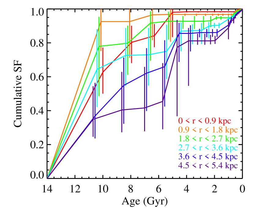
Figure 6.— Cumulative star formation (i.e., fraction of stars formed vs. age of galaxy) for all radial bins for ANGST data. Bin edges have been offset to avoid overlapping error bars.

We can use the SFH to infer the past structure of the disk. There is evidence for “inside-out” growth (Figure 4), as early star formation was more prominent in the inner disk. These trends are quantified in Figure 6, where we plot the cumulative SFH. Cumulative plots are presented at the full resolution of the CMD fit, since changes in SFR due to uncertainties typically occur in adjacent time bins and thus have a very small effect on the cumulative SFH. The outer parts of the disk formed a greater fraction of their stars at recent times than the inner parts of the disk, consistent with the “inside-out” growth scenario. However, even the outer regions are fairly old, with $\sim 75$% of stars formed by 4 Gyr ago.

We emphasize that when we refer to our “outer” disk observations in this paper, the galactocentric distances are still within 5.4 kpc for a galaxy that has been shown to extend to at least 14 kpc (Bland-Hawthorn et al., 2005). Therefore, the reader should keep in mind that all distinctions between “inner” and “outer” we can make with our data are still within what some might consider the “inner” regions of NGC 300.

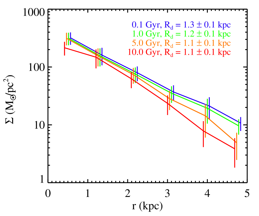
Figure 7.— Stellar surface density versus radius for multiple time bins. Points have been offset from one another by 0.05 kpc to avoid overlapping error bars. To compare this surface density with one assuming a Kroupa (2001) IMF, one should divide by 1.5.

We can also infer past stellar surface density if we assume that the majority of stars formed within the radial bin in which they are currently found (see §4.2.3). We calculate the stellar mass in each radial bin that formed before a given time by summing all the mass formed up to that time in the derived SFH. For the purposes of calculating stellar surface density we require a uniform set of time bins for all observed regions, so we choose a coarse binning scheme of 4–100 Myr, 100 Myr–1 Gyr, 1–5 Gyr, 5–10 Gyr, and 10–14 Gyr. The resulting surface mass density profile is shown in Figure 7. We omit the most recent time bin from the plot, as the surface density has not changed significantly in the past 100 Myr. The stellar surface density has changed more substantially in the outer regions of the disk than in the central regions.

For each time bin, we fit an exponential disk model to derive the scale length of the disk; the results of these fits are shown in Table 3. The scale length increased slightly over the galaxy’s history, from $1.1\pm 0.1$ kpc at early times to $1.3\pm 0.1$ kpc by 1 Gyr ago. However, our error bars are also consistent with no scale length evolution. A predominantly old disk is in contrast to the dramatic changes in scale length than has been seen in M33 or has been inferred from in situ studies of disk evolution at high redshift (e.g., Trujillo & Pohlen, 2005; Barden et al., 2005; Azzollini et al., 2008). M33 has been shown to have a scale length that increases by nearly a factor of 2 inside the disk break (Williams et al., 2009a), in agreement with the predictions of Mo et al. (1998). Although M33 is a near twin of NGC 300 in mass and morphology, NGC 300 is different in that it lacks a disk break in its exponential profile (Bland-Hawthorn et al., 2005) and is much more isolated than M33.

The value for the scale length derived by summing over the stellar mass formed in the derived SFH agrees remarkably well with the scale length for the $K$-band stellar mass surface density of $1.29^{+0.02}_{-0.03}$ (Muñoz-Mateos et al., 2007). Since massive stars have a high mass-to-light ratio in the $K$-band, agreement with the scale length as traced by the stellar mass formed in the disk is expected for a galaxy dominated by old stars ($\gtrsim 5$ Gyr). Scale lengths measured at shorter wavelengths are predictably larger, since these trace younger stellar populations: 1.47 kpc in $I$ (Kim et al., 2004) and 2.17 kpc in $B_{J}$ (Carignan, 1985, scaled to a distance of 2.0 Mpc). M33 has a similar scale length in the $K$-band of 1.4 (Muñoz-Mateos et al., 2007). In the outer fields of M33 (4–6 kpc, or $\sim 3$–4 scale lengths), only $\sim 20$% of the stars formed by 8 Gyr ($z\sim 1$), whereas in NGC 300, 50-70% of stars in the equivalent outer bins had formed by this time. Thus, the disk of NGC 300 appears to be older overall than M33. If NGC 300 experienced significant inside-out growth, it may have happened earlier than we are sensitive to with CMD fitting.

Figure 8 shows the cumulative SFH for all of NGC 300 out to 5.4 kpc. For each radial bin, we assumed the observed SFH was characteristic of the entire annulus, and summed stellar mass formed over all radial bins. Overall, $\sim 75$% of stars in this portion of NGC 300 formed by 8 Gyr ago.

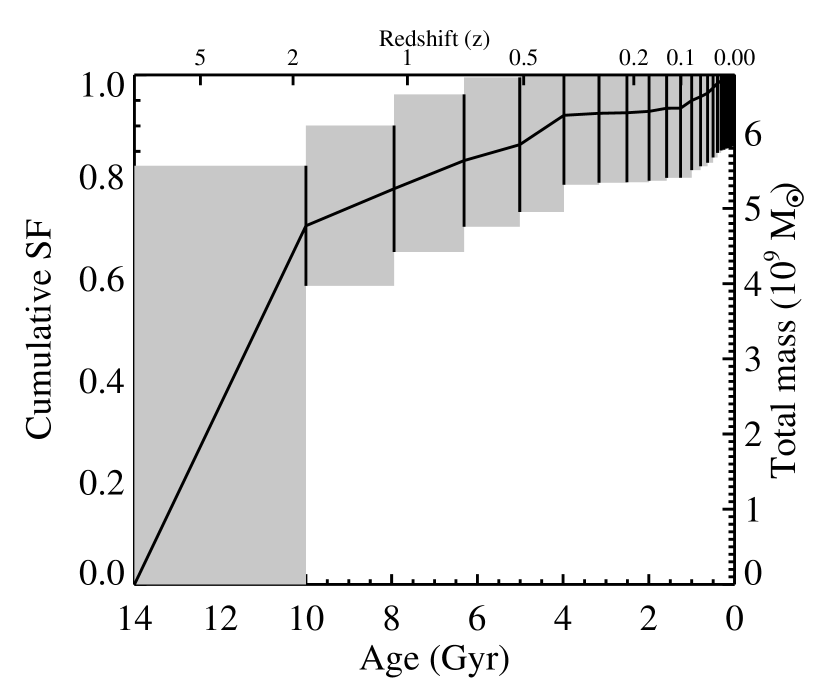
Figure 8.— Cumulative star formation for the entire galaxy out to 5.4 kpc. Shaded region indicates uncertainty.

4.2. Complicating Effects

4.2.1 Photometric Depth

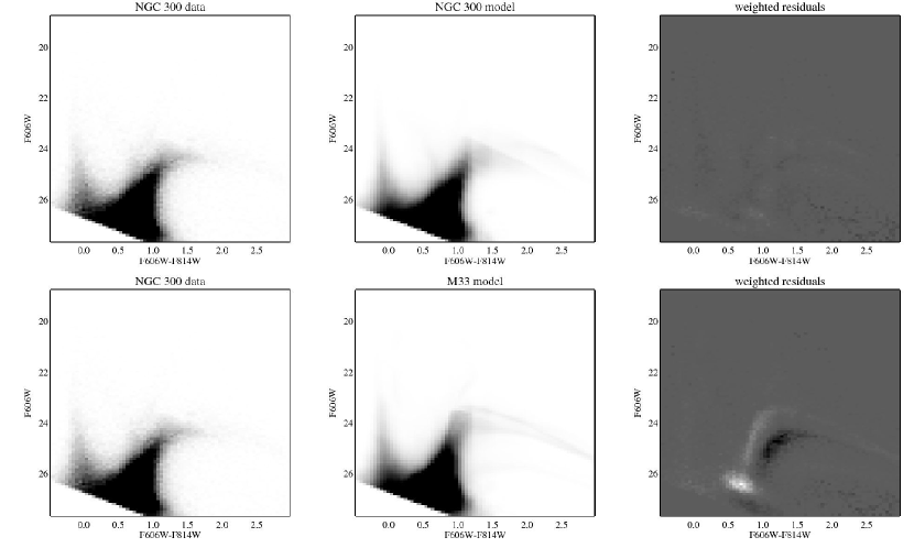
Figure 9.— Top panels: results of fitting model CMDs to the NGC 300 data. Left to right: NGC 300 binned CMD, best fit CMD to the NGC 300 data as found by MATCH, weighted residuals ((data - model)/Poisson noise). Bottom panels: results of fitting a synthetic CMD created from the SFH of the M33 field at $\sim 2.5$ kpc to the NGC 300 CMD at 1.8–2.7 kpc. Left to right: NGC 300 binned CMD, best fit CMD to the M33 data, weighted residuals. The grayscale is defined as (NGC 300 data) - (M33 model)/(Poisson noise), with darker areas being higher values (i.e. black areas show where there are more stars in NGC 300 and white areas show where there are more stars in M33). NGC 300 has a redder RGB and a fainter red clump, which is consistent with an older, more metal-rich stellar population.

Since the red clump is not resolved in the crowded inner regions, the central SFH (older than $\sim 1$ Gyr) is less certain (see §3.2), and could possibly affect our scale length derivation. As an alternative, we fit an exponential profile to only the outer four radial bins, and found essentially the same results as the fit to all the regions, albeit with larger error bars. Thus the crowded inner regions are not significantly affecting the scale lengths we derive.

To further investigate whether the SFH found for M33 is consistent with the observed stellar populations of NGC 300, we constructed model CMDs from the M33 SFHs (Williams et al., 2009a) using the photometry statistics of our NGC 300 data. For each radial bin in NGC 300, we used the SFH from the observed field in M33 that most closely matched in radius. We ran MATCH on the NGC 300 data while enforcing the M33 SFH model, scaling the SFH overall so that the number of stars produced by the model was equivalent to the number of stars observed in NGC 300. In all cases, there were substantial residuals and an obvious mismatch between the NGC 300 data and M33 SFH model.

Figure 9 compares the original MATCH fit to the NGC 300 $1.8<r<2.7$ kpc radial bin with the results of fitting the M33 model for 2.5 kpc to the same data. The top series of panels shows the MATCH fit to the NGC 300 data, along with the weighted residuals (data minus model divided by Poisson noise). Residuals for the best fitting model are very small. The bottom series of panels shows the M33 model CMD at this radius, along with the (very substantial) weighted residuals. We present this radial bin as an example; residuals were comparably large in other bins. Figure 8 in Williams et al. (2009b) demonstrates the effect of age and metallicity on the red clump and asymptotic giant branch (AGB) bump: higher metallicity gives redder colors and fainter magnitudes, while older ages result in an even stronger push towards fainter magnitudes. As shown in Figure 9, the RGB is redder in NGC 300 than in M33, and the red clump is fainter, consistent with an older, more metal-rich stellar population. This comparison confirms that the NGC 300 data is not consistent with an M33-like SFH, but rather that NGC 300 formed the majority of its stars much earlier than M33.

4.2.2 Extinction

Given what appear to be dusty regions visible toward the center of NGC 300 (Figure 2), it is possible that differential extinction may be a factor for all ages of stars. Our SFH derivation accounts for differential extinction of young stars ($<100$ Myr), but if there are dust lanes present, differential extinction could affect older stellar populations as well. Roussel et al. (2005) studied extinction in Hii regions in NGC 300 and found values for A(H$\alpha$) ranging from 0.15 to 1.06. While we expect the Hii regions to contain predominantly young stars, we can use their estimates as a rough guide for assessing extinction. In MATCH, the differential extinctions for young stars and for the stellar population in general are set by two different parameters, with the total extinction for young stars randomly assigned up to the sum of these two values. Given that we set the maximum extinction for young stars to be 0.5, if we additionally supply a value for all stars of 0.5, the young stars would receive extinction roughly in the range observed by Roussel et al. (2005).

We experimented with adding extinction parameters from 0.1 to 0.5 mag, meaning that each star is randomly assigned an extinction from zero to an upper limit of the extinction parameter. We found that the fit quality decreased with the amount of differential extinction added. In the central bin, where the presence of dust is clearly visible, this difference was minimal: up to 4%. In the remaining bins, the fit was up to 25–40% worse. For the central bin, the next best fit after no additional differential extinction is when this parameter is set at 0.2 magnitudes, so we recalculated the surface density at each time bin using up to 0.2 mag of additional extinction for only the central bin. Within the error bars, the scale length evolution remained the same.

4.2.3 Radial Stellar Migration

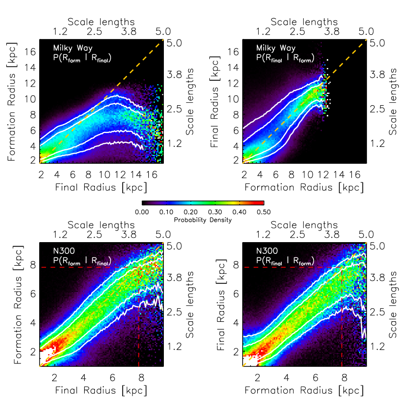
Figure 10.— Probability of migration, for MW model (top) and N300 model (bottom). Left-hand panels show, for a star at a given $R_{final}$, the probability that it formed at $R_{form}$. Right-hand panels show, for a star at a given $R_{form}$, the probability that it will end up at $R_{final}$. Contours show 50% and 75% probability. The red dashed lines in the N300 panels show the radial extent (in scale lengths) of NGC 300 studied in the current work. Yellow dashed lines show one-to-one correspondence between formation and final radii, i.e. the expected position with no migration. The N300 model shows less migration than the MW model.

Wielen (1977) suggested that substantial migration among the stars in a disk galaxy is expected, and Sellwood & Binney (2002) showed that transient spirals can provide an efficient mechanism to redistribute stars radially. Recently, Roškar et al. (2008) have reproduced this phenomenon in simulations of growing disks. Therefore, the radius at which stars are observed may not be the radius at which they formed (e.g., Wielen et al., 1996). According to Roškar et al. (2008), migration effects become more important with increasing radius, in terms of the fraction of stellar mass that is composed of migrated vs. in-situ stars. In their Milky Way-analogue model, migration significantly influenced the surface density beyond $\sim 2$ scale lengths. This suggests that the three outer radial bins in NGC 300 may contain stars that have migrated from nearer the center of the galaxy. Migration of stars from the inner to the outer disk could potentially erase the signature of inside-out growth in NGC 300, because radial bins could be contaminated by stars that did not actually form within them. If NGC 300 has had more substantial migration than M33, that could explain the discrepancy between the scale length evolution of the two galaxies. On the other hand, both M33 and NGC 300 are significantly less massive than the disks used in the Roškar et al. (2008) simulations, so the effect of radial mixing may be less severe, due to weaker spiral structure.

To examine the effects of migration in NGC 300, we ran an $N$-body simulation of a disk galaxy designed to be similar in mass and angular momentum to NGC 300. The mass at 11.8 kpc (assuming a distance of 2.0 Mpc to NGC 300) was measured to be $2.4\times 10^{10}$ $M_{\sun}$ by Puche et al. (1990) using velocity measurements from H$\alpha$. However, the disk of NGC 300 actually extends significantly farther than this (e.g., Bland-Hawthorn et al., 2005). We estimate the total mass of NGC 300, including baryonic and non-baryonic mass, to be $\sim$$10^{11}$ $M_{\sun}$ for the purposes of the simulation.

To estimate the spin parameter $\lambda$, we use the formula derived by Hernandez & Cervantes-Sodi (2006):

$$\lambda=21.8\frac{R_{d}/{\rm kpc}}{(V_{d}/{\rm km\ s}^{-1})^{3/2}},$$ (1)

where $R_{d}$ is the disk scale length and $V_{d}$ is the rotation velocity of a flat rotation curve. The $I$-band scale length of NGC 300 was measured by Kim et al. (2004) as $R_{d}=1.47$ kpc, and the velocity of $V_{d}=93.4\pm 8.2$ km s^-1 was measured by Puche et al. (1990) with Hi observations. Putting these values in equation 1, we find that for NGC 300, $\lambda\approx 0.0355$. The Milky Way model (MW) uses a total mass of $10^{12}$ $M_{\sun}$ and a spin of $\lambda\approx 0.039$. Both models are evolved to 10 Gyr; the scale lengths of the two models at the end of 10 Gyr are 1.9 kpc and 3.5 kpc for N300 and MW respectively.

Comparing the results of the simulated NGC 300 with the Milky Way-sized galaxy from Roškar et al. (2008), we find that the effect of radial migration is substantially reduced in the smaller galaxy. In Figure 10, we show the probabilities of migration for the Milky Way model (top) and the NGC 300 model (bottom). The left-hand panels should be interpreted as, “if a star is currently at $R_{final}$, what is the probability that it formed at $R_{form}$?” The right-hand panels, conversely, show “if a star forms at $R_{form}$, what is the probability that it will end up at $R_{final}$?” In all panels, probability is indicated by color, with redder colors meaning higher probabilities. In the MW model, most stars form at $<12$ kpc (top right panel), but these stars are found at radii up to 16 kpc (top left panel). Stars at all radii have a tendency to end up farther out than where they formed. In the N300 model, however, most stars are found near their birth radii.

Figure 10 shows that particles in the N300 model undergo much less radial migration than those in the more massive MW model. Since migration occurs when stars scatter off disk asymmetries such as spiral arms (Sellwood & Binney, 2002), weaker spiral structure reduces the probability of migration. A disk must remain kinematically cool to sustain recurrent transient spirals (Sellwood & Carlberg, 1984), and the only way to cool a stellar disk is by star formation, which repopulates circular orbits with young stars. Hence, if the majority of a disk is old, as in NGC 300, we can expect that it experienced radial redistribution early in its evolution, but not in recent years. Because our time resolution at old times is poor, we would not be sensitive to such early evolution.

In contrast to NGC 300, the majority of stars in M33 formed more recently (Williams et al., 2009a), so M33 may have experienced more migration in recent times. M33’s interaction with M31 may also have driven enhanced spiral structure, which in turn drives more migration (e.g, Quillen et al., 2009). NGC 300 is in a much more isolated environment. These factors combined suggest that one would expect M33 to have experienced more migration than NGC 300, not less.

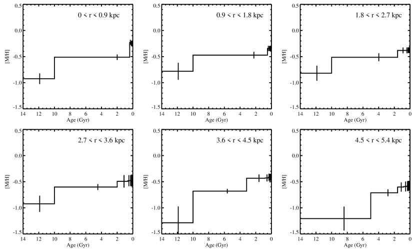
Figure 11.— Mean metallicities corresponding to SFHs in Figure 4. Errors are calculated as in Figure 4.

In summary, while migration will tend to erase the signature of disk growth, it is not the only way to obtain scale lengths which do not evolve as a function of age of stellar population. From our modeling, we can surmise that mass is an important factor in the extent of radial migration, with less massive systems experiencing less redistribution. Consequently, the lack of scale length evolution in NGC 300 is attributable to a factor other than radial migration, in this case most likely the rapid early growth of the disk.

Further evidence that NGC 300 has not experienced much migration comes from the kinematics of the globular cluster systems. Olsen et al. (2004) and Nantais et al. (2008) found that the globular clusters in NGC 300 had kinematics matching that of the Hi disk, indicating that their present location is where they formed. Since both heating and migration are caused by spiral arms, this finding would suggest a lack of migration as well. In a more massive galaxy, NGC 253, asymmetric drift of the globular clusters indicates stronger radial diffusion. This result agrees with the prediction of the models described here in suggesting that more massive galaxies experience greater migration. The old globular clusters with disk kinematics in NGC 300 also fits with the interpretation that the majority of stars formed early.

4.2.4 Comparison with M33’s scale length evolution

We considered whether the NGC 300 data is consistent with the stronger scale length evolution seen in M33, such that the observed weaker evolution is due solely to the shallower depth of the NGC 300 CMDs. In other words, if M33 were at the distance of NGC 300, would the results of Williams et al. (2009a) be recoverable? Unlike the test in §4.2.1, in which we saw that the SFH of M33 is not compatible with the NGC 300 data, here we are looking at the effect of depth on the M33 data.

We calculated photometry of the M33 data using only one 1300s exposure in $F606W$ and $F814W$ for each of the ACS fields analyzed in Williams et al. (2009a). When deriving the SFH we considered only the portion of the CMD that was 2 magnitudes above the 50% completeness limit, to mimic the effect of placing M33 at the distance of NGC 300. We found a smaller scale length evolution than Williams et al. (2009a), with the scale length increasing from $1.0\pm 0.2$ kpc at 8 Gyr to $1.3\pm 0.1$ kpc at 0.1 Gyr. In contrast, Williams et al. (2009a) found an increase of $1.0\pm 0.1$ at 10 Gyr to $1.8\pm 0.1$ at 0.6 Gyr with the deeper data. Thus, the reduced depth can lead to an underestimate of the scale length evolution; it may be possible that the evolution of NGC 300 is comparably dramatic to that seen in M33, but that we are not sensitive to it due to the shallower depth of the NGC 300 data. On the other hand, the inferred evolution for the shallower M33 data is still somewhat larger than we observed in NGC 300. We emphasize that the difference in mean age of the two galaxies, as seen in §4.2.1, is still secure.

Table 2 ANGST data: ages, SFRs, and metallicities for each radial bin

Radius	Area	Age	SFR	$\rm{[M/H]}$
(kpc)	(kpc2)	(Gyr)	($M_{\sun}$ yr-1 kpc-2)
0–0.9	1.40	0.004–0.079	$0.0110\pm 0.0013$	$-0.24\pm 0.05$
		0.079–0.13	$0.0069\pm 0.0009$	$-0.24\pm 0.05$
		0.13–0.25	$0.0054\pm 0.0011$	$-0.25\pm 0.05$
		0.25–0.40	$0.0511\pm 0.0109$	$-0.23\pm 0.05$
		0.40–10	$0.0219\pm 0.0085$	$-0.51\pm 0.05$
		10–14	$0.1098\pm 0.0291$	$-0.92\pm 0.10$
0.9–1.8	2.53	0.004–0.079	$0.0189\pm 0.0023$	$-0.34\pm 0.05$
		0.079–0.13	$0.0117\pm 0.0018$	$-0.34\pm 0.05$
		0.13–0.20	$0.0100\pm 0.0009$	$-0.34\pm 0.05$
		0.20–0.32	$0.0102\pm 0.0012$	$-0.35\pm 0.05$
		0.32–0.50	$0.0410\pm 0.0107$	$-0.34\pm 0.05$
		0.50–10	$0.0041\pm 0.0036$	$-0.47\pm 0.06$
		10–14	$0.1358\pm 0.0488$	$-0.78\pm 0.16$
1.8–2.7	1.98	0.004–0.079	$0.0089\pm 0.0015$	$-0.38\pm 0.05$
		0.079–0.13	$0.0069\pm 0.0016$	$-0.38\pm 0.05$
		0.13–0.20	$0.0077\pm 0.0008$	$-0.38\pm 0.05$
		0.20–0.32	$0.0081\pm 0.0005$	$-0.38\pm 0.05$
		0.32–0.50	$0.0162\pm 0.0019$	$-0.38\pm 0.06$
		0.50–1.6	$0.0064\pm 0.0009$	$-0.38\pm 0.06$
		1.6–10	$0.0046\pm 0.0043$	$-0.51\pm 0.08$
		10–14	$0.0452\pm 0.0141$	$-0.82\pm 0.14$
2.7–3.6	1.90	0.004–0.079	$0.0124\pm 0.0024$	$-0.47\pm 0.11$
		0.079–0.13	$0.0074\pm 0.0008$	$-0.48\pm 0.11$
		0.13–0.20	$0.0054\pm 0.0010$	$-0.48\pm 0.11$
		0.20–0.40	$0.0045\pm 0.0005$	$-0.48\pm 0.11$
		0.40–0.63	$0.0090\pm 0.0012$	$-0.48\pm 0.11$
		0.63–2.0	$0.0049\pm 0.0025$	$-0.49\pm 0.12$
		2.0–10	$0.0035\pm 0.0029$	$-0.60\pm 0.06$
		10–14	$0.0162\pm 0.0060$	$-0.92\pm 0.16$
3.6–4.5	1.83	0.004–0.100	$0.0050\pm 0.0009$	$-0.41\pm 0.07$
		0.100–0.158	$0.0034\pm 0.0004$	$-0.42\pm 0.07$
		0.158–0.25	$0.0035\pm 0.0004$	$-0.42\pm 0.07$
		0.25–0.40	$0.0044\pm 0.0008$	$-0.41\pm 0.07$
		0.40–0.79	$0.0045\pm 0.0005$	$-0.43\pm 0.07$
		0.79–3.2	$0.0022\pm 0.0011$	$-0.43\pm 0.07$
		3.2–10	$0.0042\pm 0.0031$	$-0.68\pm 0.04$
		10–14	$0.0052\pm 0.0025$	$-1.29\pm 0.31$
4.5–5.4	1.35	0.004–0.079	$0.0027\pm 0.0006$	$-0.58\pm 0.10$
		0.079–0.158	$0.0015\pm 0.0002$	$-0.58\pm 0.09$
		0.158–0.25	$0.0017\pm 0.0003$	$-0.58\pm 0.10$
		0.25–0.40	$0.0014\pm 0.0002$	$-0.58\pm 0.09$
		0.40–0.79	$0.0022\pm 0.0005$	$-0.59\pm 0.10$
		0.79–1.6	$0.0033\pm 0.0003$	$-0.60\pm 0.09$
		1.6–5.0	$0.0023\pm 0.0012$	$-0.71\pm 0.07$
		5.0–14	$0.0011\pm 0.0005$	$-1.21\pm 0.23$

Table 3 Fits to the surface density and metallicity gradient

Age	$\Sigma_{0}$	$R_{d}$	$Z_{0}$	$\Delta Z/\Delta r$
(Gyr)	($M_{\sun}$ pc-2)	(kpc)		(kpc-1)
0.004	$506.946\pm 106.331$	$1.21\pm 0.10$	$-0.23\pm 0.05$	$-0.072\pm 0.019$
0.1	$507.602\pm 106.786$	$1.21\pm 0.10$	$-0.23\pm 0.05$	$-0.075\pm 0.019$
1.0	$513.618\pm 110.948$	$1.16\pm 0.10$	$-0.40\pm 0.05$	$-0.057\pm 0.018$
5.0	$586.142\pm 129.738$	$0.95\pm 0.09$	$-0.52\pm 0.05$	$-0.078\pm 0.020$
10	$443.474\pm 110.079$	$0.97\pm 0.10$	$-0.89\pm 0.11$	$-0.059\pm 0.049$

4.3. Metallicity

In most models of galaxy evolution, the buildup of a stellar population is accompanied by an increase in the mean stellar metallicity. Outside the Milky Way, metallicity is often measured only for the youngest stellar populations, using either Hii regions or atmospheres of A and B stars (with the latter method being used only for the nearest galaxies). Here we discuss the present-day metallicity structure of NGC 300 and compare it to its past evolution as derived from stellar populations.

4.3.1 Present Day Metallicity

A radial metallicity gradient for NGC 300 in the gas and young stars has been reported by a number of authors (Pagel et al., 1979; Webster & Smith, 1983; Edmunds & Pagel, 1984; Deharveng et al., 1988; Zaritsky et al., 1994; Urbaneja et al., 2005; Kudritzki et al., 2008; Bresolin et al., 2009). All these studies found that metallicity is highest in the center and decreases toward larger radii, although the overall metallicity depends on the calibration method used. The results best suited for comparison with metallicities derived from our stellar populations are those of Urbaneja et al. (2005) and Kudritzki et al. (2008), since they determine metallicities using stellar spectroscopy of individual young A and B stars from the galactic center out to $\sim 6.8$ kpc, and are thus measuring the stellar, rather than gas-phase, metallicity gradient. The best-fit abundance gradient of Kudritzki et al. (2008) is

$$[Z]=(-0.06\pm 0.09)-(0.078\pm 0.021)r$$ (2)

where $r$ is radius in kpc (assuming the distance used in this paper of 2.0 Mpc) and [Z] is an average metallicity based on a combination of multiple abundance measurements (mostly Fe, Ti, and Cr lines). We adopt Equation 2 as the best estimate of the present-day metallicity gradient. The Hii-region metallicities from temperature-sensitive emission lines presented in Bresolin et al. (2009) also agree remarkably well with these stellar metallicities.

4.3.2 Metallicity Evolution from HST Data

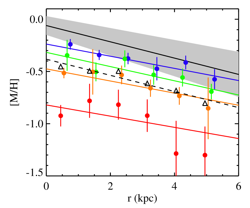
Figure 12.— Solid black line: best-fit metallicity gradient obtained from young massive stars (Kudritzki et al., 2008), with shaded region showing uncertainties. Blue circles are metallicities measured from our CMDs in each radial bin at the present day (i.e., the mean metallicity for the past 100 Myr); green, orange, and red circles are metallicities for the 1–5 Gyr, 5–10 Gyr, and 10–14 Gyr bins, respectively. Solid lines of corresponding colors show the best linear fit for each set of points. Errors are calculated as in Figure 4. Mean metallicities for the entire stellar population are shown with black triangles, with a dashed black line showing the best linear fit. Points have been offset in radius to avoid overlapping error bars.

The metallicity gradient measured in young stars by Kudritzki et al. (2008) can be compared to the present-day metallicities inferred from the observed stellar populations. The CMDs contain information on the metallicities as well as the ages of stars, especially for stars off the main sequence (Gallart et al., 2005). A full suite of isochrones with varying age and metallicity is used to fit each CMD, so that in the final SFH each time bin is associated with a particular metallicity. The full metallicity history for all radial bins is shown in Figure 11. Uncertainties in the metallicity may result from several factors: 1) an age-metallicity degeneracy in the RGB, 2) photometric errors in the CMD, 3) uncertainties in the reddening, 4) uncertainties in modeling stars on the instability strip, and 5) errors in the isochrones, especially for supergiants and AGB stars. We address these uncertainties by constraining the metallicity not to decrease significantly with time, which eliminates unphysical solutions to the SFH.

We tested the effect of this parameter by deriving the SFH without it as well. Not constraining the metallicity results in lower [M/H] values for intermediate age stars (1–10 Gyr), especially in the most crowded regions, but the effect on the SFR is minimal. The trends in SFH reported in this paper do not depend on whether or not the metallicity constraint is enforced.

The derived SFH from the ANGST data reproduces a metallicity gradient in the present-day metallicity (4–100 Myr) time bin. In Figure 12 we show the Kudritzki et al. (2008) metallicity gradient along with our derived metallicity gradient. Fit parameters for the linear fits are given in Table 3. The MATCH-derived present-day metallicities are generally consistent with the observed values within the error bars, although the metallicities are all systematically low and fall near the minimum value in the observed uncertainty range. The mean metallicities of the entire population are lower as well, as would be expected for a stellar population that built up gradually over $\sim 10$ Gyr. However, the mean stellar metallicity still shows a radial gradient at all epochs.

Since the color of the main sequence is not significantly affected by metallicity, our CMD-fitting code may not be sensitive to a metallicity increase at very recent times. The metallicities we find are therefore a lower limit on the current values (at least in the central regions where the infall of unenriched gas is assumed to have ended). This insensitivity is especially true in the innermost radial bins, in which the low current SFRs and the effects of crowding make the present-day metallicity especially difficult to determine. Not coincidentally, these values fall more significantly below the Kudritzki et al. (2008) results than do the values for the outer disk.

The change in the metallicity gradient over time can be seen in the mean metallicity derived during multiple time bins, also shown in Figure 12. Stellar population ages of 4–100 Myr, 1–5 Gyr, 5–10 Gyr, and 10–14 Gyr are shown. (The metallicity values for age 100 Myr – 1 Gyr are essentially identical to the present-day values.) Results of linear fits to the gradients are presented in Table 3. Outside 2 kpc, the slope of the metallicity gradient has remained fairly constant over time, with the overall metallicity increasing. In the central 2 kpc, we see a significant metallicity increase from the 10–14 Gyr bin to the 5–10 Gyr bin, which corresponds to the epoch when significant star formation activity was taking place in the galactic center.

4.3.3 Comparison with M33’s metallicity

Figure 12 shows that NGC 300 has both a significant radial metallicity gradient and a significant increase in metallicity with time. Although we constrained the metallicity not to decrease with time, there was no barrier to its remaining constant in deriving the SFHs, or to its taking arbitrary slopes with radius. In contrast, M33 has a shallower gradient and metallicity which has remained nearly constant with time (Magrini et al., 2009, Holtzman et al. 2009, in prep.).

These results are consistent with chemical evolution models. Ongoing star formation in M33 may indicate gas infall, which can dilute the metallicity, keeping it constant with time despite the continuing enrichment from star formation. In contrast, NGC 300 formed a small fraction of its stars at late times, which may indicate a less important role for ongoing gas accretion, and thus chemical evolution that behaves more like a closed box. This may also be a counterexample to the “downsizing” model, since NGC 300 is a fairly low-mass disk galaxy.

5. Conclusions

We have presented resolved stellar photometry of 3 HST/ACS fields in a continuous radial strip from the center of NGC 300 to 5.4 kpc, as well as additional archival fields scattered throughout the disk. For both the ANGST (continuous) and archival fields, we have divided the stars into 6 radial bins of width 0.9 kpc and used CMD-fitting to derive the SFH in each bin. We can resolve the red clump in the majority of the radial bins. We find that the disk of NGC 300 has a dominant old population throughout the observed region: looking at the disk as a whole, $\sim$80% of stars are older than 6 Gyr. However, the outer parts of the disk have a higher percentage of young stars than the inner parts, consistent with inside-out growth. In the inner regions, $>90$% of the stars are older than 6 Gyr, while in the outermost radial bin ($4.5<5.4$ kpc), only $\sim$40% of stars are this old. Comparison of formation and final positions of stars in an $N$-body simulation of an NGC 300-like galaxy indicates that the effects of migration should not be substantial in a galaxy of this size.

We calculated the surface density profile of the disk at each time step by summing over the stellar mass formed and fitting the profile to derive the corresponding scale lengths. According to inside-out growth, the scale length of the disk should increase with time. While we found this to be the case, the increase is relatively small, from $\sim 1.1$ to $\sim 1.3$ kpc over the lifetime of the disk. In contrast, the scale lengths of M33 found with an identical method show a much greater increase, from 1.0 kpc to 1.8 kpc (Williams et al., 2009a), more in line with the theoretical predictions of Mo et al. (1998).

Although M33 is nearly a twin to NGC 300 in Hubble type and mass, there are differences between the two galaxies which may be related to their different SFHs. The primary difference in morphology is the presence of a disk break in M33. Breaks have been shown to be extremely common in disk galaxies (Pohlen & Trujillo, 2006), and M33 is no exception, with a break at 8 kpc (Ferguson et al., 2007). The scale length increase seen by Williams et al. (2009a) only holds inside the disk break; outside the break the opposite trend is seen, with a decreasing scale length with time. In contrast, NGC 300 is unusual in that it has no disk break out to at least 14 kpc (Bland-Hawthorn et al., 2005). Sánchez-Blázquez et al. (2009) suggest that pure exponential profiles may be a feature of galaxies that have undergone less radial mixing, which is consistent with our analysis in §4.2.3 that NGC 300 has undergone relatively little recent migration.

Environmental factors may also be important, as NGC 300 is isolated from other large galaxies while M33 appears to be interacting with M31 (Braun & Thilker, 2004; Bekki, 2008; McConnachie et al., 2009; Putman et al., 2009). An influx of gas onto M33 in recent times may have triggered star formation in the outskirts of M33 and contributed to the growth of the disk.

Finally, we note that despite the unbroken exponential profile of NGC 300, it is not without features in the very outer disk (beyond the extent of our observations): Vlajić et al. (2009) find a change in the abundance gradient at $\sim 10$ kpc. They propose two possible explanations for the upturn in the gradient: radial mixing, which we conclude is unlikely to be the sole effect based on the simulation presented in §4.2.3, and an accretion scenario in which the outer regions of the disk form stars later and become enriched, flattening the gradient. We suggest that additional HST observations of resolved stars farther out in NGC 300 would provide useful constraints on the total disk scale length and evolution.

From our derived SFH for NGC 300, we find a present-day metallicity gradient roughly consistent with observational results (Kudritzki et al., 2008; Bresolin et al., 2009). Additionally, we find that the metallicity has increased with time in all radial bins, suggesting a lack of infall of unenriched gas. This is broadly consistent with our finding that the majority of stars in NGC 300 formed prior to 6 Gyr ago, as more recent gas infall would likely have triggered more enhanced recent star formation. As M33 has been shown to have little evolution in metallicity and more of its stars formed recently, it may have experienced more gas infall at later times. Despite the visual similarities between these two galaxies, they seem to have markedly different histories.

Appendix A Archival Data

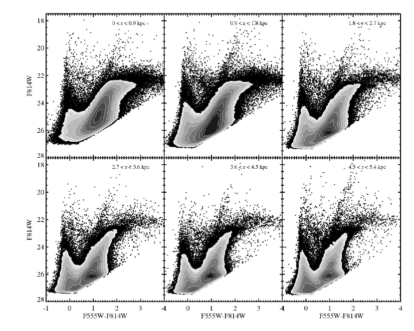
Figure 13.— CMDs of radial bins from archival data. Quality cuts are identical to those described in Figure 3.

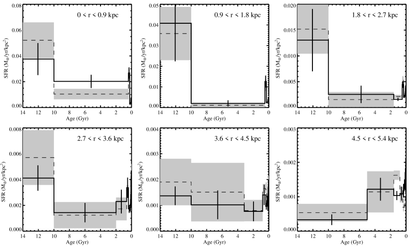
Figure 14.— Lifetime SFHs of radial bins from archival data (solid lines). Errors are calculated as in Figure 4. For comparison, the ANGST SFHs are shown as dashed lines, with uncertainties shown as shaded regions.

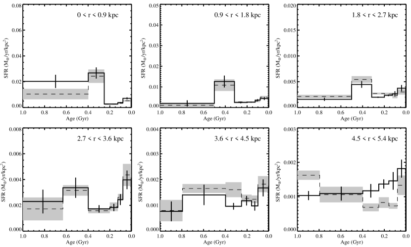
Figure 15.— Recent ($<1$ Gyr) SFHs of radial bins from archival data (solid lines). Errors are calculated as in Figure 4. For comparison, the ANGST SFHs are shown as dashed lines, with uncertainties shown as shaded regions.

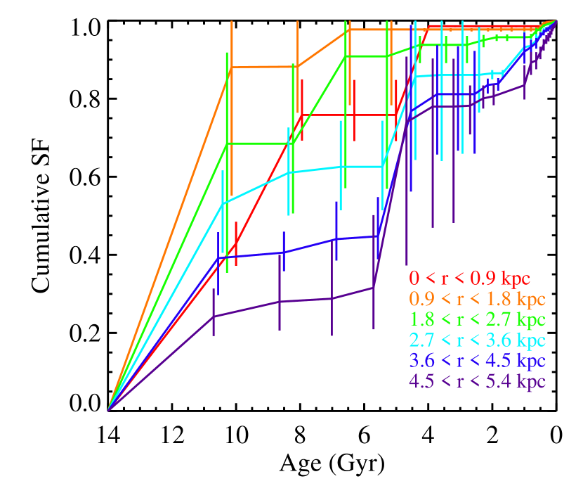
Figure 16.— Cumulative star formation for all radial bins for archival data. Bin edges have been offset to avoid overlapping error bars.

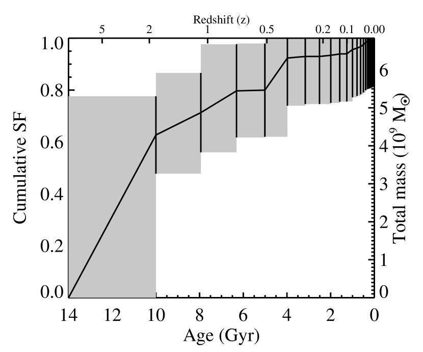
Figure 17.— Cumulative star formation for the entire galaxy out to 5.4 kpc. Shaded region indicates uncertainty.

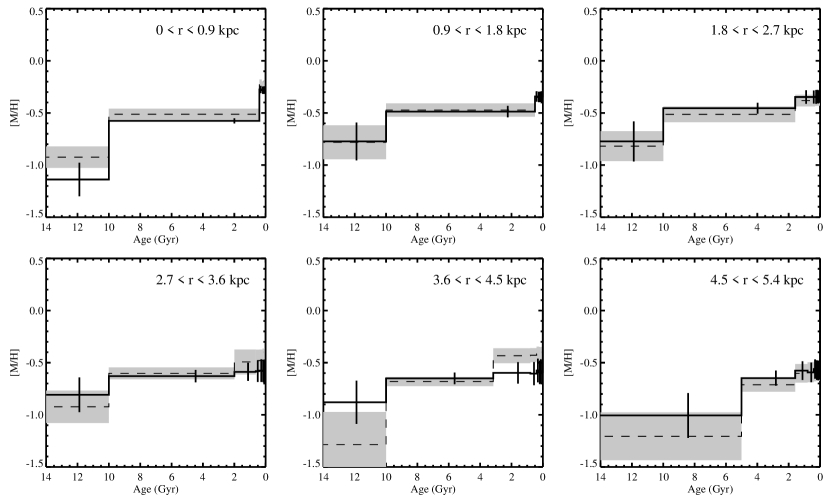
Figure 18.— Mean metallicities corresponding to SFHs in Figure 14. Solid lines are archival data, and dashed lines (with shaded uncertainties) are ANGST data. Errors are calculated as in Figure 4.

Table 4 Archival data: ages, SFRs, and metallicities for each radial bin

Radius	Area	Age	SFR	$\rm{[M/H]}$
(kpc)	(kpc2)	(Gyr)	($M_{\sun}$ yr-1 kpc-2)
0–0.9	1.89	0.004–0.079	$0.0201\pm 0.0023$	$-0.28\pm 0.03$
		0.079–0.13	$0.0108\pm 0.0010$	$-0.28\pm 0.04$
		0.13–0.25	$0.0078\pm 0.0006$	$-0.28\pm 0.04$
		0.25–0.40	$0.0760\pm 0.0122$	$-0.28\pm 0.03$
		0.40–10	$0.0575\pm 0.0145$	$-0.58\pm 0.03$
		10–14	$0.1065\pm 0.0352$	$-1.14\pm 0.16$
0.9–1.8	3.41	0.004–0.079	$0.0223\pm 0.0037$	$-0.34\pm 0.05$
		0.079–0.13	$0.0183\pm 0.0026$	$-0.35\pm 0.05$
		0.13–0.20	$0.0133\pm 0.0013$	$-0.35\pm 0.05$
		0.20–0.32	$0.0124\pm 0.0021$	$-0.35\pm 0.05$
		0.32–0.50	$0.0645\pm 0.0146$	$-0.34\pm 0.05$
		0.50–10	$0.0102\pm 0.0076$	$-0.49\pm 0.05$
		10–14	$0.2088\pm 0.0944$	$-0.77\pm 0.18$
1.8–2.7	2.47	0.004–0.079	$0.0139\pm 0.0023$	$-0.34\pm 0.06$
		0.079–0.13	$0.0098\pm 0.0019$	$-0.35\pm 0.06$
		0.13–0.20	$0.0087\pm 0.0006$	$-0.34\pm 0.06$
		0.20–0.32	$0.0074\pm 0.0004$	$-0.35\pm 0.07$
		0.32–0.50	$0.0165\pm 0.0024$	$-0.35\pm 0.06$
		0.50–1.6	$0.0059\pm 0.0011$	$-0.35\pm 0.06$
		1.6–10	$0.0094\pm 0.0062$	$-0.46\pm 0.05$
		10–14	$0.0483\pm 0.0223$	$-0.77\pm 0.19$
2.7–3.6	2.71	0.004–0.079	$0.0162\pm 0.0029$	$-0.58\pm 0.11$
		0.079–0.13	$0.0100\pm 0.0017$	$-0.59\pm 0.11$
		0.13–0.20	$0.0074\pm 0.0011$	$-0.58\pm 0.11$
		0.20–0.40	$0.0070\pm 0.0012$	$-0.58\pm 0.11$
		0.40–0.63	$0.0137\pm 0.0032$	$-0.58\pm 0.10$
		0.63–2.0	$0.0093\pm 0.0037$	$-0.59\pm 0.09$
		2.0–10	$0.0058\pm 0.0031$	$-0.63\pm 0.06$
		10–14	$0.0167\pm 0.0040$	$-0.81\pm 0.17$
3.6–4.5	3.94	0.004–0.100	$0.0099\pm 0.0019$	$-0.59\pm 0.11$
		0.100–0.16	$0.0058\pm 0.0011$	$-0.58\pm 0.11$
		0.16–0.25	$0.0070\pm 0.0011$	$-0.59\pm 0.11$
		0.25–0.40	$0.0057\pm 0.0008$	$-0.58\pm 0.11$
		0.40–0.79	$0.0083\pm 0.0023$	$-0.61\pm 0.11$
		0.79–3.2	$0.0045\pm 0.0023$	$-0.60\pm 0.10$
		3.2–10	$0.0060\pm 0.0033$	$-0.65\pm 0.06$
		10–14	$0.0081\pm 0.0021$	$-0.88\pm 0.21$
4.5–5.4	4.68	0.004–0.079	$0.0128\pm 0.0018$	$-0.57\pm 0.09$
		0.079–0.16	$0.0103\pm 0.0018$	$-0.58\pm 0.09$
		0.16–0.25	$0.0096\pm 0.0009$	$-0.57\pm 0.09$
		0.25–0.40	$0.0082\pm 0.0014$	$-0.56\pm 0.09$
		0.40–0.79	$0.0077\pm 0.0014$	$-0.59\pm 0.09$
		0.79–1.6	$0.0073\pm 0.0009$	$-0.58\pm 0.09$
		1.6–5.0	$0.0085\pm 0.0023$	$-0.65\pm 0.07$
		5.0–14	$0.0023\pm 0.0011$	$-1.01\pm 0.21$

In this section we present the results of analyzing archival fields in NGC 300 (see §2.1) in the same manner as the ANGST data. CMDs for the archival data are shown in Figure 13. The quality cuts used for selecting stars were identical to those described for the ANGST data in §2.2. Although the archival fields are not radially aligned, the stars in these fields can be sorted into the same 6 bins as the new observations. These fields are not evenly spaced in radius, as shown in Figure 1, and were placed on regions of high current star formation. We include only stars up to a galactocentric distance of 5.4 kpc, the radial extent of the ANGST data.

As with the ANGST data, we fixed the distance for these SFH derivations at $m-M=26.43$. The results of the fits were combined into time bins identical to those used for the ANGST data. For the archival data, mean extinction values for each bin are, from inner to outer: $A_{V}=0.30\pm 0.05,0.20\pm 0.05,0.10\pm 0.05,0.10\pm 0.05,0.10\pm 0.05,0.13\pm 0.07$. The higher extinction values for the archival data are likely due to the location of these fields in regions of higher star formation, which should correspond with increased dust content that affects older stars as well. Indeed, Roussel et al. (2005) studied extinction in NGC 300 and found that extinction is variable for young clusters.

Reassuringly, the SFH from the archival data, shown in Figures 14 and 15, is very similar to that derived from the ANGST data, despite the different filters and depths. Cumulative SFHs for archival data divided into radial bins are shown in Figure 16, and integrated for the whole galaxy in Figure 17. Metallicities are shown in Figure 18. Table 4 gives the full SFH for the archival data.

References

- Azzollini et al. (2008) Azzollini, R., Trujillo, I., & Beckman, J. E. 2008, ApJ, 679, L69
- Barden et al. (2005) Barden, M. et al. 2005, ApJ, 635, 959
- Bekki (2008) Bekki, K. 2008, MNRAS, 390, L24
- Bertelli et al. (1994) Bertelli, G., Bressan, A., Chiosi, C., Fagotto, F., & Nasi, E. 1994, A&AS, 106, 275
- Bland-Hawthorn et al. (2005) Bland-Hawthorn, J., Vlajić, M., Freeman, K. C., & Draine, B. T. 2005, ApJ, 629, 239
- Boissier & Prantzos (1999) Boissier, S., & Prantzos, N. 1999, MNRAS, 307, 857
- Braun & Thilker (2004) Braun, R., & Thilker, D. A. 2004, A&A, 417, 421
- Bresolin et al. (2009) Bresolin, F., Gieren, W., Kudritzki, R.-P., Pietrzyński, G., Urbaneja, M. A., & Carraro, G. 2009, ApJ, 700, 309
- Bresolin et al. (2005) Bresolin, F., Pietrzyński, G., Gieren, W., & Kudritzki, R.-P. 2005, ApJ, 634, 1020
- Brook et al. (2006) Brook, C. B., Kawata, D., Martel, H., Gibson, B. K., & Bailin, J. 2006, ApJ, 639, 126
- Burkert et al. (1992) Burkert, A., Truran, J. W., & Hensler, G. 1992, ApJ, 391, 651
- Butler et al. (2004) Butler, D. J., Martínez-Delgado, D., & Brandner, W. 2004, AJ, 127, 1472
- Carignan (1985) Carignan, C. 1985, ApJS, 58, 107
- Chiappini et al. (1997) Chiappini, C., Matteucci, F., & Gratton, R. 1997, ApJ, 477, 765
- Corbelli & Salucci (2000) Corbelli, E., & Salucci, P. 2000, MNRAS, 311, 441
- Dalcanton et al. (2009) Dalcanton, J. J. et al. 2009, ApJS, 183, 67
- Deharveng et al. (1988) Deharveng, L., Caplan, J., Lequeux, J., Azzopardi, M., Breysacher, J., Tarenghi, M., & Westerlund, B. 1988, A&AS, 73, 407
- Dolphin (2000) Dolphin, A. E. 2000, PASP, 112, 1383
- Dolphin (2002) —. 2002, MNRAS, 332, 91
- Edmunds & Pagel (1984) Edmunds, M. G., & Pagel, B. E. J. 1984, MNRAS, 211, 507
- Ferguson et al. (2007) Ferguson, A., Irwin, M., Chapman, S., Ibata, R., Lewis, G., & Tanvir, N. 2007, Resolving the Stellar Outskirts of M31 and M33 (Island Universes - Structure and Evolution of Disk Galaxies), 239
- Ford et al. (1998) Ford, H. C. et al. 1998, in Society of Photo-Optical Instrumentation Engineers (SPIE) Conference Series, Vol. 3356, Society of Photo-Optical Instrumentation Engineers (SPIE) Conference Series, ed. P. Y. B. . J. B. Breckinridge, 234–248
- Gallart et al. (1999) Gallart, C., Freedman, W. L., Aparicio, A., Bertelli, G., & Chiosi, C. 1999, AJ, 118, 2245
- Gallart et al. (2005) Gallart, C., Zoccali, M., & Aparicio, A. 2005, ARA&A, 43, 387
- Gieren et al. (2005) Gieren, W., Pietrzyński, G., Soszyński, I., Bresolin, F., Kudritzki, R.-P., Minniti, D., & Storm, J. 2005, ApJ, 628, 695
- Girardi et al. (2002) Girardi, L., Bertelli, G., Bressan, A., Chiosi, C., Groenewegen, M. A. T., Marigo, P., Salasnich, B., & Weiss, A. 2002, A&A, 391, 195
- Girardi et al. (2008) Girardi, L. et al. 2008, PASP, 120, 583
- Harris & Zaritsky (2004) Harris, J., & Zaritsky, D. 2004, AJ, 127, 1531
- Hernandez & Cervantes-Sodi (2006) Hernandez, X., & Cervantes-Sodi, B. 2006, MNRAS, 368, 351
- Hernandez et al. (1999) Hernandez, X., Valls-Gabaud, D., & Gilmore, G. 1999, MNRAS, 304, 705
- Holtzman et al. (1999) Holtzman, J. A. et al. 1999, AJ, 118, 2262
- Karachentsev et al. (2003) Karachentsev, I. D. et al. 2003, A&A, 404, 93
- Kim et al. (2004) Kim, S. C., Sung, H., Park, H. S., & Sung, E.-C. 2004, Chinese Journal of Astronomy and Astrophysics, 4, 299
- Kroupa (2001) Kroupa, P. 2001, MNRAS, 322, 231
- Kroupa (2002) —. 2002, Science, 295, 82
- Kudritzki et al. (2008) Kudritzki, R.-P., Urbaneja, M. A., Bresolin, F., Przybilla, N., Gieren, W., & Pietrzyński, G. 2008, ApJ, 681, 269
- Larson (1976) Larson, R. B. 1976, MNRAS, 176, 31
- MacArthur et al. (2009) MacArthur, L. A., González, J. J., & Courteau, S. 2009, MNRAS, 395, 28
- Magrini et al. (2009) Magrini, L., Stanghellini, L., & Villaver, E. 2009, ApJ, 696, 729
- Marigo et al. (2008) Marigo, P., Girardi, L., Bressan, A., Groenewegen, M. A. T., Silva, L., & Granato, G. L. 2008, A&A, 482, 883
- Matteucci & Francois (1989) Matteucci, F., & Francois, P. 1989, MNRAS, 239, 885
- McConnachie et al. (2009) McConnachie, A. W. et al. 2009, Nature, 461, 66
- Mo et al. (1998) Mo, H. J., Mao, S., & White, S. D. M. 1998, MNRAS, 295, 319
- Muñoz-Mateos et al. (2007) Muñoz-Mateos, J. C., Gil de Paz, A., Boissier, S., Zamorano, J., Jarrett, T., Gallego, J., & Madore, B. F. 2007, ApJ, 658, 1006
- Naab & Ostriker (2006) Naab, T., & Ostriker, J. P. 2006, MNRAS, 366, 899
- Nantais et al. (2008) Nantais, J. B., Huchra, J. P., Barmby, P., & Olsen, K. A. G. 2008, ArXiv e-prints
- Olsen et al. (2004) Olsen, K. A. G., Miller, B. W., Suntzeff, N. B., Schommer, R. A., & Bright, J. 2004, AJ, 127, 2674
- Pagel et al. (1979) Pagel, B. E. J., Edmunds, M. G., Blackwell, D. E., Chun, M. S., & Smith, G. 1979, MNRAS, 189, 95
- Pohlen & Trujillo (2006) Pohlen, M., & Trujillo, I. 2006, A&A, 454, 759
- Puche et al. (1990) Puche, D., Carignan, C., & Bosma, A. 1990, AJ, 100, 1468
- Putman et al. (2009) Putman, M. E. et al. 2009, ApJ, 703, 1486
- Quillen et al. (2009) Quillen, A. C., Minchev, I., Bland-Hawthorn, J., & Haywood, M. 2009, MNRAS, 397, 1599
- Rizzi et al. (2006) Rizzi, L., Bresolin, F., Kudritzki, R.-P., Gieren, W., & Pietrzyński, G. 2006, ApJ, 638, 766
- Roussel et al. (2005) Roussel, H., Gil de Paz, A., Seibert, M., Helou, G., Madore, B. F., & Martin, C. 2005, ApJ, 632, 227
- Roškar et al. (2008) Roškar, R., Debattista, V. P., Quinn, T. R., Stinson, G. S., & Wadsley, J. 2008, ApJ, 684, L79
- Sakai et al. (2004) Sakai, S., Ferrarese, L., Kennicutt, Jr., R. C., & Saha, A. 2004, ApJ, 608, 42
- Salpeter (1955) Salpeter, E. E. 1955, ApJ, 121, 161
- Sánchez-Blázquez et al. (2009) Sánchez-Blázquez, P., Courty, S., Gibson, B. K., & Brook, C. B. 2009, MNRAS, 398, 591
- Schlegel et al. (1998) Schlegel, D. J., Finkbeiner, D. P., & Davis, M. 1998, ApJ, 500, 525
- Sellwood & Binney (2002) Sellwood, J. A., & Binney, J. J. 2002, MNRAS, 336, 785
- Sellwood & Carlberg (1984) Sellwood, J. A., & Carlberg, R. G. 1984, ApJ, 282, 61
- Skillman et al. (2003) Skillman, E. D., Tolstoy, E., Cole, A. A., Dolphin, A. E., Saha, A., Gallagher, J. S., Dohm-Palmer, R. C., & Mateo, M. 2003, ApJ, 596, 253
- Spergel et al. (2007) Spergel, D. N. et al. 2007, ApJS, 170, 377
- Trujillo & Pohlen (2005) Trujillo, I., & Pohlen, M. 2005, ApJ, 630, L17
- Urbaneja et al. (2005) Urbaneja, M. A. et al. 2005, ApJ, 622, 862
- Vila-Costas & Edmunds (1992) Vila-Costas, M. B., & Edmunds, M. G. 1992, MNRAS, 259, 121
- Vlajić et al. (2009) Vlajić, M., Bland-Hawthorn, J., & Freeman, K. C. 2009, ApJ, 697, 361
- Webster & Smith (1983) Webster, B. L., & Smith, M. G. 1983, MNRAS, 204, 743
- White & Frenk (1991) White, S. D. M., & Frenk, C. S. 1991, ApJ, 379, 52
- Wielen (1977) Wielen, R. 1977, A&A, 60, 263
- Wielen et al. (1996) Wielen, R., Fuchs, B., & Dettbarn, C. 1996, A&A, 314, 438
- Williams et al. (2009a) Williams, B. F., Dalcanton, J. J., Dolphin, A. E., Holtzman, J., & Sarajedini, A. 2009a, ApJ, 695, L15
- Williams et al. (2009b) Williams, B. F. et al. 2009b, AJ, 137, 419
- Williams et al. (2009c) —. 2009c, ArXiv e-prints
- Zaritsky (1999) Zaritsky, D. 1999, AJ, 118, 2824
- Zaritsky et al. (2002) Zaritsky, D., Harris, J., Thompson, I. B., Grebel, E. K., & Massey, P. 2002, AJ, 123, 855
- Zaritsky et al. (1994) Zaritsky, D., Kennicutt, Jr., R. C., & Huchra, J. P. 1994, ApJ, 420, 87