The Isospin Dependence Of The Nuclear Equation Of State Near The Critical Point

Abstract

We discuss experimental evidence for a nuclear phase transition driven by the different concentration of neutrons to protons. Different ratios of the neutron to proton concentrations lead to different critical points for the phase transition. This is analogous to the phase transitions occurring in ⁴He-³He liquid mixtures. We present experimental results which reveal the N/A (or Z/A) dependence of the phase transition and discuss possible implications of these observations in terms of the Landau Free Energy description of critical phenomena.

Nuclei are quantum Fermi systems which exhibit ma-
ny interesting features which depend on temperature and density. At zero temperature and ground state density, nuclei are charged quantum drops, i.e. they have a Fermi motion pres due to their quantum nature, and nucleons interact through a short range attractive force and the long range Coulomb repulsions among the constituent protons. In the absence of the Coulomb force, the Nuclear Hamiltonian is perfectly symmetric for exchange of protons and neutrons apart from a small but NOT insignificant difference between the proton and neutron masses. This symmetry is revealed by similar energy levels in mirror nuclei, i.e. nuclei with the same mass number A but opposite numbers of neutrons, N, and protons, Z. Of course this feature is observed for relatively small systems because the Coulomb energy is small pres . Analogous to the properties of mirror nuclei, we could expect that if we study nuclei at finite temperatures, T, and low densities, $\rho$, then, if the Coulomb force is not important, the invariance under exchange of protons to neutrons might lead to important and interesting consequences. In fact, since the fundamental Hamiltonian of nuclei is invariant under exchange of N with Z (apart from Coulomb effects), we could expect that such an invariance should be manifested only at high T (disordered state), while there is a spontaneous symmetry breaking at lower T (ordered state). That means that in symmetric nuclear matter at high T, the state with fragments having $N=Z$ defines the minimum of the free energy, i.e. symmetric fragments such as deuterons and alphas would be favored at low density  huang ; land . On the other hand, there could be a symmetry breaking favoring $N\neq Z$ at lower T. In this case fragments near a (first order) phase transition might prefer either a neutron or proton rich configuration. There might even be a more interesting situation, suggested by the present data, the existence of a line of first order phase transitions  huang which terminates in a tri-critical point. For such a line the free energy has three equal minima: one with N=Z and the other two for $N\neq Z$. Thus a phase transition is driven by the difference in isospin concentration of the fragments $m=(N-Z)/A$. In this paper we will discuss data which clearly demonstrate that m is an order parameter of the phase transition. Its conjugate field huang which we indicate with H, is due to the chemical potential difference between protons and neutrons of the emitting source at the density and temperature reached during a collision between heavy ions prl ; huang10_1 . We also note that the phase transition has a strong resemblance to that observed in superfluid mixtures of liquid ⁴He-³He near the $\lambda$ point. In both systems, changing the concentration of one of the components of the mixture, changes the characteristics of the Equation Of State (EOS) huang ; land .

In recent times a large body of experimental evidence has been interpreted as demonstrating the occurrence of a phase transition in finite nuclei at temperatures (T) of the order of 6 MeV and at densities, $\rho$, less than half of the normal ground state nuclear density wci . Even though strong signals for a first and a second-order phase transition have been found wci ; bon00 , there remain a number of open questions regarding the Equation of State of nuclear matter near the critical point. In particular the roles of Coulomb, symmetry, pairing and shell effects have yet to be clearly delineated.

Theoretical modeling indicates that a nucleus excited in a collision expands nearly adiabatically until it is close to the instability region thus the expansion is isentropic siem . At the last stage of the expansion the role of the Coulomb force becomes very important. In fact, without the Coulomb force, the system would require a much larger initial compression and/or temperature in order to enter the instability region and fragment. The Coulomb force acts as an external piston, giving the system an ‘extra push’ to finally fragment. These features are clearly seen in Classical Molecular Dynamics (CMD) simulations of expanding drops with and without a Coulomb field belk95 ; dorso . The expansion with the Coulomb force included is very slow in the later stage and nearly isothermal.

Even though at high T and small $\rho$ the nucleus behaves as a classical fluid, the analogy to classical systems should not be overemphasized as, in the (T,$\rho$) region of interest, the nucleus is still a strongly interacting quantum system. In particular the ratio of T to the Fermi energy at the (presumed) critical point is still smaller than 1 which suggests that the EOS of a nuclear system is quite different from the classical one. To date this expected difference has not been well explored mor ; wci ; dago ; mas ; nat ; ala ; maria .

The paper is organized as follows: in the next section we discuss the experimental setup in detail. This is followed by a description of the data analysis and a discussion in terms of the Landau O($m^{6}$) free energy. We, then derive some critical exponents and the EOS corresponding to possible scenarios suggested by our data in terms of the Fisher model of fragmentation. Finally we draw some conclusions and suggest possible future work.

I Experimental Details

The experiment was performed at the K-500 superconducting cyclotron facility at Texas $A\&M$ University. ^64,70Zn and ⁶⁴Ni beams were incident on ^58,64Ni, ^112,124Sn, ¹⁹⁷Au and ²³²Th targets at 40 A MeV. Intermediate mass fragments (IMF) were detected by a detector telescope placed at 20^o. The telescope consisted of four Si detectors. Each Si detector had 5cm $\times$ 5cm area. The thicknesses were 129, 300, 1000 and 1000 $\mu$m. All Si detectors were segmented into four sections and each quadrant had a 5^o acceptance in polar and azimuthal angles. The fragments were detected at average angles of 17.5^o $\pm$ 2.5^o and 22.5^o $\pm$ 2.5^o. Typically 6-8 isotopes were clearly identified for a given Z up to Z=18 with an energy threshold of 4-10 A MeV, using the $\Delta$E-E technique for any two consecutive detectors. The $\Delta$E-E spectrum was linearized by an empirical code based on a range-energy table. In the code, isotopes are identified by a parameter $Z_{Real}$. For the isotopes with A=2Z, $Z_{Real}$ = Z is assigned and other isotopes are identified by interpolating between them. The energy spectrum of each isotope was extracted by gating on lines corresponding to the individual identified isotopes. In order to compensate for the imperfectness of the linearization, actual gates for isotopes were made on the 2D plot of $Z_{Real}$ versus energy. The multiplicity of each isotope was evaluated from the extracted energy spectra, using a moving source fit at the two given angles. Since the energy spectra of some isotopes have very low statistics, the following procedure was adopted for the fits. Using a single source with a smeared source velocity around half of the beam velocity, the fit parameters were first determined from the energy spectrum summed over all isotopes for a given Z, assuming A=2Z. Then assuming that the shape of the velocity spectrum is the same for all isotopes for a given Z. All parameters except the normalizing multiplicity parameter were assumed to be the same as for the summed spectrum. The multiplicity for a given isotope was then derived by normalizing the standard spectrum to the observed spectrum for that isotope.

In order to evaluate the back ground contribution to the extracted multiplicity a two Gaussian fit to each isotope peak was used with a linear background. The second Gaussian (about 10$\%$ of the height of the first one) was added to reproduce the valleys between isotopes. This component was attributed to the reactions of the isotope in the Si detector. The centroid of the main Gaussian was set to the value calculated from the range-energy table within a small margin. The final multiplicity of an isotope with Z $>$ 2 was obtained by correction of the multiplicity evaluated form the moving source fit for the ratio between the sum of the two Gaussian yields and the linear background.

The yields of light charged particles (Z $\leq$ 2) in coincidence with IMFs were also measured using 16 single crystal CsI(Tl) detectors of 3cm thickness set around the target. The light output from each detector was read by a photo multiplier tube. The pulse shape discrimination method was used to identify p, d, t, h and $\alpha$ particles. The energy calibration for these particles were performed using Si detectors (50 -300 $\mu$m) in front of the CsI detectors in separate runs. The yield of each isotope was evaluated, using a moving source fit. Three sources (projectile-like(PLF), nucleon-nucleon-like(NN) and target-like (TLF)) were used. The NN-like sources have source velocities of about a half of the beam velocity. The parameters were searched globally for all 16 angles. Detailed procedures of the data analysis are also given in refs. huang10_2 ; chen10 .

Special care has been taken for ⁸He identification. All He isotopes are identified in the Si telescope, using the $\Delta$E-E technique, in a narrow energy range. When a proton and an $\alpha$ hit the same quadrant and when both of them stop in the E detector, their $\Delta$E-E points overlap with those of ⁸He. Since the multiplicities of protons and alphas are about three orders of magnitude larger than that of ⁸He, the contribution of accidental events becomes significant, especially for the reaction systems with lower numbers of neutrons, in which ⁸He production is suppressed. Since Z=1 $\Delta$E-E spectra are not available in this experiment, $\Delta$E-E for Z $\leq 3$ were measured in a separate run. Using the light charged particle multiplicity extracted from the 16 CsI detectors, the accidental events were simulated for each reaction for the observed $\alpha$ yield in the $\Delta$E-E spectra in this experiment, the solid angle of the quadrant and the multiplicity of Z=1 particles. In order to minimize the accidental events, the runs with a low beam intensity were selected in each reaction. Typical linearized $Z_{Real}$ spectra with these accidentals are shown in Fig.(1) for ⁷⁰Zn + ²³²Th (N/Z $\sim$ 1.5) and ⁶⁴Ni + ¹¹²Sn ( N/Z $\sim$ 1.25). As one can see, the $Z_{real}$ values for the accidental events of proton and $\alpha$ pileup is nearly identical to that of ⁸He, while ⁶He is clearly identified. The contributions from d + $\alpha$ and t + $\alpha$ are also reasonably consistent with the observed background yields. A significant excess of ⁸He yield beyond the accidentals is only observed for the reaction systems with the ¹²⁴Sn, ¹⁹⁷Au and ²³²Th targets. After the correction of the accidental contributions, the multiplicities of ⁶He and ⁸He were calculated using the source fit parameters obtained for Li isotopes.

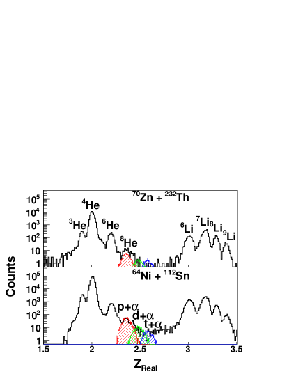
Figure 1: Typical $Z_{Real}$ spectra for He and Li isotopes. Accidental events are generated only for p, d, t +$\alpha$ and shown separately by shaded histograms as indicated.

II Data Analysis

The key factor in our analysis is the value $I=N-Z$ of the detected fragments. A plot of the yield versus mass number when I=0 displays a power law behavior with yields decreasing as $A^{-\tau}$  min ; prl . This is shown in Fig.(2) for the ⁶⁴Ni+¹²⁴Sn case at 40 MeV/nucleon. In the figure we have made separate fits for odd-odd (open symbols) or even-even(filled symbols) nuclei. As seen, different exponents $\tau$ appear which suggests that pairing is playing a role in the dynamics  pres , leading to higher yields for even-even nuclei.

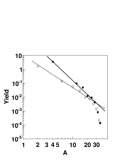
Figure 2: Mass distribution for the ⁶⁴Ni+¹²⁴Sn system at 40 MeV/nucleon for I=0. The lines are power law fits with exponents $2.3\pm 0.02$ (odd-odd nuclei, dashed line), and $3.4\pm 0.06$ (even-even nuclei, full line) respectively.

The observation of the power law behavior suggests that the mass distributions may be discussed in terms of a modified Fisher model bon00 ; min :

$$Y=y_{0}A^{-\tau}e^{-\beta\Delta\mu A},$$ (1)

where y₀ is a normalization constant, $\tau=2.3$ is a critical exponent  bon00 , $\beta$ is the inverse temperature and $\Delta\mu=F(I/A)$ is the free energy per particle, $F$, near the critical point. Recall that in general, the free energy is a function of the mass A (volume), $A^{2/3}$(surface) and the chemical composition $m$ of the fragments and possibly pairing. The region we are studying in this paper seems near the critical point for a liquid gas phase transition (volume and surface equal to zero) but modified by $m=\frac{I}{A}$. Because of this modification we can observe different features of the transition such as a first order phase transition driven by $m$, the order parameter.

We begin our analysis by noting that the Fisher free energy is usually written in terms of the volume and the surface of a drop undergoing a (second order) phase transition fisher . Our data indicate that those terms are not important in the present case bon00 as we will show more in detail below. If they are negligible this suggests that we are near the critical point for a liquid gas phase transition. Because we have two different interacting fluids, neutrons and protons, the transition becomes more complex and more interesting than in a single component liquid. Experiments at different energies might display a free energy which depends on all these factors. If we accept that $F$ is dominated by the symmetry energy we can make the approximation that $F(I/A)=E_{sym}=25(I/A)^{2}$ MeV/A, i.e. the symmetry energy of a nucleus in its ground state pres . We will use this relationship in order to infer an approximate value of the temperature of the system. However, we stress that in actuality, F(I/A) is a function of density, temperature and all other relevant quantities near the critical point. According to the Fisher equation given above, we can compare all systems on the same basis by normalizing the yields and factoring out the power law term. For this purpose we have chosen to normalize the yield data for each system to the ¹²C yield ($I=0$) in that system, i.e. we define a ratio:

$$R=\frac{YA^{\tau}}{Y(^{12}C)12^{\tau}}.$$ (2)

The normalized ratios for the system ⁶⁴Ni + ⁶⁴Ni at 40 MeV/nucleon are plotted as a function of the (ground state) symmetry energy in Fig.(3), bottom panel. The data display an exponential decrease with increasing symmetry energy, except for the isotopes for which $I=0$. The yields of these I = 0 isotopes are of course not sensitive to the symmetry energy but rather to the Coulomb and pairing energies and possibly to shell effects. A fit to the exponentially decreasing portion of the data using the ground state symmetry energy gives an ‘apparent temperature’ T of 6.0 MeV. This value of T would be the real one if only the symmetry energy is important, if entropy can be neglected, if $a_{sym}=25$ MeV (the g.s. symmetry energy coefficient value) and if secondary decay effects are negligible. In general we expect that the symmetry energy coefficient is density and temperature dependent. Further, secondary decay processes may modify the primary fragment distributions huang10_2 ; chen10 . we will discuss these questions in the framework of the Landau free energy approach below. We stress that the appearance of two branches in Fig.3 (bottom), indicates that the total free energy must contain an odd power term in (I/A) at variance with the common expression for the ground state symmetry energy. For reference in the top part of Fig.(3) we have plotted the ratio versus the total ground state binding energy of the fragments. No clear correlations are observed which might suggest that the symmetry energy dominates the process.

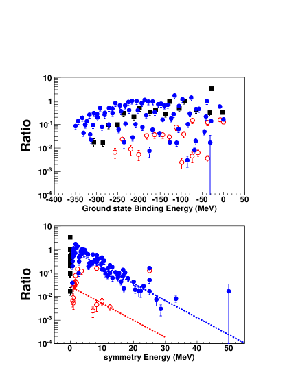
Figure 3: Ratio versus fragments ground state binding energy (top panel) and symmetry energy (bottom panel) for the ⁶⁴Ni + ⁶⁴Ni case at 40 MeV/nucleon. $a_{s}ym$=25 MeV is used. The $I<0$ and $I>0$ ($I=0$)isotopes are indicated by the open and full circles respectively (full squares). The dashed lines (bottom panel) are fits using a ground state symmetry energy, Eq.1, and a ‘temperature’ of 6 MeV. Notice that the given experimental ⁸He yield is the upper limit.

It is surprising that such a scaling appears as a function of the symmetry energy only. In fact we might wonder about the role of the Coulomb energy if we accept that surface and volume terms give negligible contribution. In figure 4 we have plotted the same normalized ratios as a function of the quantity $\alpha E_{coul}+\beta E_{sym}$, $\alpha$ and $\beta$ are arbitrary parameters given in the figure and $E_{coul}=0.7Z(Z-1)A^{-1/3}$ is the Coulomb contribution to the ground state energy of the nucleus. We see from the figure that by decreasing the relative contribution of the Coulomb energy compared to the symmetry energy the scaling appears. This implies that the Coulomb energy is much less important than the symmetry energy near the critical point, which suggests that either the density dependence of those two terms is different or that, at the time of formation the fragments are strongly deformed, reducing the Coulomb effect. Such deformations have been seen in CMD calculations of fragmentation  bon00 .

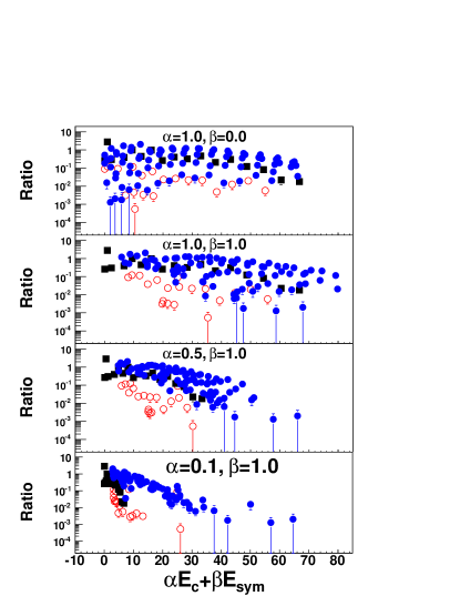
Figure 4: Ratio versus symmetry energy + Coulomb energy for the ⁶⁴Ni + ¹²⁴Sn case at 40 MeV/nucleon. The panels from top to bottom are for different combinations of the symmetry and Coulomb energy. The $I<0$ and $I>0$ ($I=0$)isotopes are indicated by the open and full circles respectively (full squares).

To further explore the role of the relative nucleon concentrations we plot in Fig.(5) the quantity $\frac{F}{T}=-\frac{ln(R)}{A}$ versus $m=(I/A)$, the difference in neutron and proton concentration of the fragment. As expected the normalized yield ratios depend strongly on m.

Pursuing the question of phase transition we can perform a fit to these data within the generalized Landau free energy description huang . In this approach the ratio of the free energy to the temperature is written in terms of an expansion:

$$\frac{F}{T}=\frac{1}{2}am^{2}+\frac{1}{4}bm^{4}+\frac{1}{6}cm^{6}-m\frac{H}{T},$$ (3)

where $m$ is an order parameter, $H$ is its conjugate variable and $a-c$ are fitting parameters  huang . We observe that the Free energy is even in the exchange of $m\rightarrow-m$, reflecting the invariance of the nuclear forces when exchanging N and Z. This symmetry is violated by the conjugate field $H$ which arises when the source is asymmetric in chemical composition. We stress that m and H are related to each other through the relation $m=-\frac{\delta F}{\delta H}$.

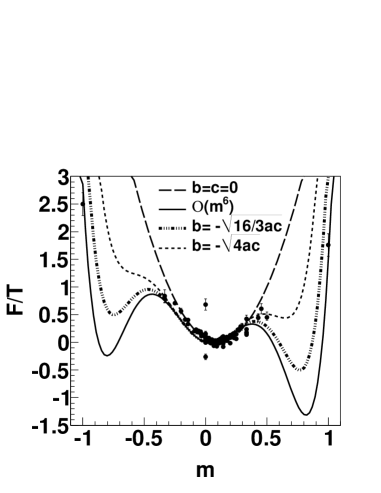
Figure 5: Free energy versus m for the case ⁶⁴Ni+²³²Th. The full line is a free fit based on Landau O($m^{6}$) free energy. The dashed-dotted-dotted-dotted line is obtained imposing in the fit $b=-\sqrt{16/3ac}$ and it is located on a line of first order phase transitions. The short dashed line corresponds to $b=-\sqrt{4ac}$, i.e. superheating. The $O(m^{2})$ case, $F/T=a(m-m_{s})^{2},$i.e. $b=c=0$, $m_{s}=0.1$, is given by the long dashed line.

The use of the Landau approach is for guidance only. While the approximation to $O(m^{4})$ does not work prl , the $O(m^{6})$ case is in good agreement with the data. This is not surprising since, if fluctuations are important, a higher order approximation to the free energy is better, i.e. gives critical exponents closer to those seen in the data and satisfies the Ginzburg criterion  huang . A free fit using Eq.3 is displayed in Fig.5 (full line). Notice the change of curvature near $m=0.3$, which incidentally is close to $m_{cn}$ of the compound nucleus. For comparison in the same figure we have displayed the $O(m^{2})$ case, i.e., $F/T=a(m-m_{s})^{2}$ ($b=c=0$) As seen in the plot last assumption also produces a reasonable fit, although it does not reproduce shoulders near m $\sim\pm$0.3. As we will discuss in more detail below the appearance of two minima for $m\neq 0$ (when $H/T=0$) might be a signature for the existence of a first order phase transition occurring in these reactions.

In general the coefficients entering the Landau free energy Eq.(3), depend on temperature, pressure or density of the source. Usually one assumes $c>0$, $a=a_{0}(\rho)(T-T_{0})$ and $b=b(T,\rho)$, where $T_{0}$ is some ‘critical’ temperature discussed below. The precise determination of these parameters determines the nuclear equation of state (NEOS) near the critical point. The data we have do not allow such a complete constraining of the NEOS but do suggest some interesting possible scenarios which we discuss below.

We begin by noting that the conjugate variable H which appears in equation (3) is determined by the chemical composition of the source. Since, in general, the source has $N\neq Z$, the extreme of $F/T$ are displaced from the values obtained when H=0. In fact if we take the first derivative of the free energy we get:

$$(\frac{F}{T})^{\prime}=am+bm^{3}+cm^{5}-\frac{H}{T}.$$ (4)

When $H/T=0$ the first derivative is zero for the following values of m  huang :

$$m_{0}=0;m^{2}_{\pm}=\frac{-b\pm\sqrt{b^{2}-4ac}}{2c}.$$ (5)

If we now assume $H\neq 0$ but small, we can expand the solutions above as $m=m_{0\pm}+\eta$ with $\eta$ small. Equating the first derivative to zero, Eq.(4), and neglecting terms $O(\eta^{2})$ we get:

$$\eta=\frac{H/T}{a+3bm_{0\pm}^{2}+5cm_{0\pm}^{4}}.$$ (6)

The shift of the minimum from $m_{0}=0$ should be given by the equation above and should be proportional to $m$ of the emitting source. We can easily check this feature in our data. In Fig.(6) we plot the values of $H/T$ obtained from the fits to our data for all systems using Eq.(3) versus $m_{cn}=(I/A)_{cn}$.

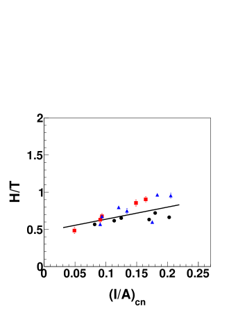
Figure 6: H/T versus (I/A) of the compound nucleus obtained from the data fit to the Landau free energy, Eq.(3). The full circles are for ⁶⁴Ni, the full triangles are for ⁷⁰Zn and the squares for ⁶⁴Zn projectiles impinging on various targets, see text.

The linear fit in Fig.6 is given by $H/T=0.47+1.6(I/A)_{cn}$ which agrees with the linear dependence of Eq.(6). However, for this fit $H/T\neq 0$ for $I_{cn}=0$ which could indicate the favoring of $N>Z$ fragments by the Coulomb field. Another possibility is that $(I/A)_{source}\propto(I/A){cn}$ which then gives $H=0$ when $I_{source}=0$. Finally we should consider that together with H also the temperature may also be changing some since the collisions are between different target-projectile combinations at the same beam energy. If the temperature were the same then the coefficients of the free energy, Eq.3, should be independent of the source size, only H/T should change. In Fig.(7) we plot the parameters a, b and c as a function of the compound nucleus $m_{cn}$. As we see there is some dependence which may reflect differences in temperature. However, we note that the error bars and fluctuations are large which may also indicate important secondary decay effects. Thus is not too so easy to draw definite conclusions.

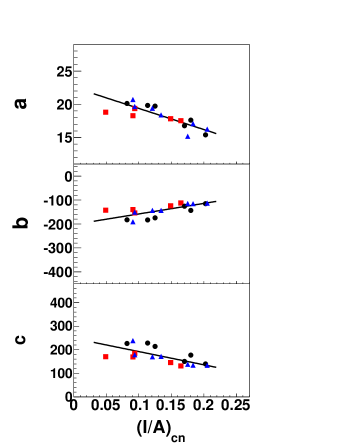
Figure 7: The parameters a,b and c versus (I/A) of the compound nucleus obtained from the data fit to the Landau free energy, Eq.(3). The symbols are like in figure 6.

Given the information on the parameters of the Landau free energy contained in figures 6 and 7 we can discuss some features regarding the NEOS. In particular for each reaction system we can estimate F/T when $H/T=0$. In figure 8 we plot this quantity versus m of the fragments for various reactions.

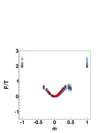
Figure 8: F/T (H/T=0) versus m of the fragments obtained from the a, b and c parameters fit to the Landau free energy, Eq.(3). Results for all experimentally investigated reactions are displayed.

The curves do not differ much suggesting that temperatures are quite similar. The fits exhibit curvature near $m=\pm 0.4$ which may suggest the presence of additional minima at larger absolute values of m. This could indicate either a first order phase transition or superheating (see below). The lack of data at very large $m$ makes it difficult to constrain the fit. However, we can study other situations of particular physical interest which arise when the relationships among the parameters a, b and c are constrained.  huang ; land ; prl :

We have considered four such cases as follows:

1) superheating. This case corresponds to $b=-\sqrt{4ac}$ and gives two minima at $m\neq 0$ and is plotted in figure 5 for the ⁶⁴Ni+²³²Th system with a short dashed line. These are not absolute minima, which occur only at $m=0$, and they correspond to metastable states. They might be observed in high quality data for collisions of more neutron rich or proton rich systems making a hot source with $m_{source}\approx\pm 0.4$. In fact if the system could be gently brought to the right temperature $T_{s}$, with the correct isotopic composition, it might stay in the minimum, i.e. more fragments of that $m$ should appear;
2) line of first order phase transition. This corresponds to the condition $b=-\sqrt{16ac/3}$ at a temperature $T_{3}$, which, if imposed on the fit of the free energy, results in the dashed-dotted-dotted-dotted line of Fig.5. This fit is of similar quality to the previous cases. Now the minima are at $m\approx 0.6$, i.e. for more neutron rich fragments due to the fact that $H/T\neq 0$. This suggests that in this situation we might produce a large number of neutron rich fragments. However, most of those fragments are probably unstable, thus coincidence measurements may be required to determine their yields. Of course this feature should become important in neutron rich stars.
3) first order phase transition. Corresponds to the case $a=0$ and determines the ‘critical temperature’ $T_{0}$ where the minimum at $m=0$ disappears and only the ones at $m\neq 0$ survive. This case is excluded by our present data. However, the fit in Fig.(5) suggests an intermediate situation between this and case (2) above.
4) line of second order phase transition, tri-critical point. Corresponds to $a=0$ and $b>0$ ($T=T_{c}$). When $b=0$ as well we have a tricritical point ($T=T_{3c}$), i.e. the point where the line of first order phase transition terminates into a second order phase transition. This case is also excluded by our data.

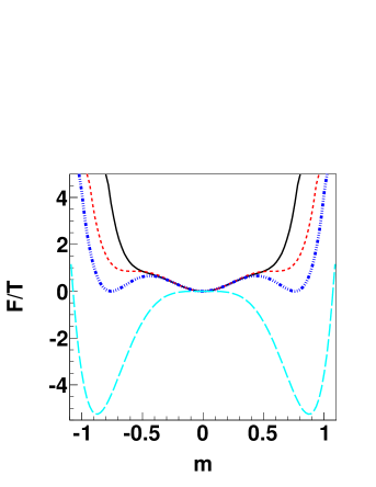
Figure 9: F/T (H/T=0) versus m of the fragments obtained from the a, b and c parameter fit to the Landau free energy, Eq.(3) for ⁶⁴Ni+²³²Th. The four curves correspond to vapor(full line), superheating(short dashed), line of first order transition(3 critical dashed-dotted-dotted-dotted line), first order phase transition(long dashed line), see text.

We can extrapolate the cases discussed above to $H/T=0$ as was done for Fig.8. In Fig.9 we plot F/T (H/T=0) (extrapolated from the data) vs. $m$. Purists will not call this the EOS but reserve that for the pressure vs. $m$ case (that we discuss below). Since H/T is zero, the curves are symmetric with respect to $m$. We see in the plot: vapor (dashed-dotted-dotted line) $T>T_{s}$, superheating $(T=T_{s})$(dotted line), a point in the line of a first order phase transition $(T=T_{3})$(dashed-dotted line) which displays three equal minima at $m_{0}$ and $m_{\pm}$, see Eq.5, the experimental data fit line(full line)$T<T_{3}$. We have also added the case $a=0$ which should be obtained at $T=T_{0}$, where the minimum at $m=0$ becomes a maximum. There is a series of cases not displayed in the figure, corresponding to the temperatures between $T_{0}$ and $T_{3}$ where $m=0$ is still a minimum but $\it{not}$ an absolute minimum. This corresponds to supercooling and might be observed in gentle collisions of $N=Z$ nuclei similarly to the superheating case.

The features in Fig.9 are reminiscent of the superfluid $\lambda$ transition observed as some ³He is added to ⁴He  huang . Pure ⁴He has a critical temperature of 2.18 K. The critical temperature for the second-order transitions decreases with increasing ³He concentration until at temperature, $T=0.867$K, a first-order transition appears. This point is known as the tri-critical point for this system. In a similar fashion, a nucleus, which can undergo a liquid-gas phase transition, should be influenced by the different neutron to proton concentrations. Thus the discontinuity observed in Fig.5 ($m=0$) could be a signature for a tri-critical point as in the ⁴He-³He case. We believe that our data, analyzed in terms of the the Landau O($m^{6}$) free energy, suggest such a feature but are not sufficient to clearly demonstrate this. Some other work campi ; gulm , also suggests that a line of critical points might be found away from its ‘canonical’ position, i.e. at the end of a first-order phase transition and, for small systems, even extending into the coexistence region.

III Critical exponents

In the fits discussed above the parameters a, b and c were left free since we do not have any particular values to fix the scale. Nevertheless, we saw in figure 8 that the free energy (H/T=0) looks very similar for the different systems. Thus the values of the fitting parameters are similar apart from a scaling factor. We can avoid unnecessary factors by defining suitable dimensionless quantities. This can be accomplished by looking at the solutions of the minima of the free energy, cf. Eq.5. In particular from the value at the minimum, $m_{+}$ we can define the following quantities ($b\neq 0$):

$$x=\frac{4ac}{b^{2}}.$$ (7)

Recalling that $a$ is related to the distance from the critical temperature while b and c should only depend on density  huang , we deduce that x is a measure of the distance $T-T_{3}$ from the critical temperature in a suitable dimensionless fashion. Similarly we can define a reduced order parameter from Eq.5:

$$y=\frac{2cm^{2}}{|b|}.$$ (8)

Thus Eq.5 can be rewritten as:

$$y=1+\sqrt{1-x}.$$ (9)

Near the critical point we know that the order parameter has a singular part that behaves in a power law fashion, thus we can define the singular part as:

$$M=\pm\sqrt{y-1}=\pm{(1-x)}^{1/4},$$ (10)

defining the temperature ‘distance’ from the critical point, $|t|=|1-x|$, immediately gives the value of a critical exponent: $\beta=\frac{1}{4}$. This exponent is very close to the accepted experimental value as is well known in the O($m^{6}$) Landau theory  huang .

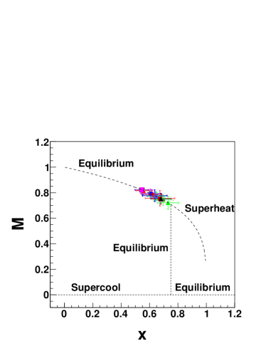
Figure 10: Order parameter versus reduced temperature for all studied systems. The dashed line is given by Eq.(10), the vertical line indicates the critical temperature $T_{3}$. To the right of this line the system is in a superheated state. Supercooling occurs on the left of the vertical line and M=0 huang .

In Fig.(10) the experimental values of M and x obtained within the Landau theory are plotted together with the equilibrium condition given by Eq.(10). Supercooling and Superheating regions, as discussed in the previous section, can be identified as well  huang .

As is the case for macroscopic systems we can now ‘turn ’ the external field H on and off. In our case this is done with a suitable choice of the colliding systems. In this way we can study the ‘EOS’ at the critical point by turning on H:

$$M=H^{1/\delta},$$ (11)

which defines the critical exponent $\delta$. In the Landau theory this exponent can be determined at the critical point where $a=b=0$. From equation (4) we easily get $\delta=5$, which is the accepted value for such a critical exponent huang . In order to exactly determine this exponent we need to bring the system to the critical point. This does not appear to be the case for our data as we saw in figure 10. Nevertheless a plot of the order parameter versus H should display a power law behavior as it is well known in macroscopic systems huang . A precise determination of the critical exponent requires the knowledge of the temperature T both above and below the critical point. This is feasible but requires precise experimental data. ¿From Eq.(6) assuming the only minimum is at m=0 we get

$$\eta=\frac{H/T}{a}.$$ (12)

The temperature (a) dependence of the order parameter shows that we are away from the critical point. Nevertheless we can study the behavior close to the critical point by suitably defining scaling forms  huang : $\frac{M}{|t|^{\beta}}=\frac{\eta}{|t|^{\beta}}$ vs. $\frac{H/T}{|t|^{\beta\delta}}$. These quantities are plotted in figure 11 and compared to magnetization data for nickel metal. The scaled magnetization is plotted versus the scaled external magnetic field huang . The nuclear data have been shifted in the region near the crossing of data above and below the critical temperature where we expect our data to be, see Fig.10. Of course it is not possible at this stage to directly compare to the macroscopic data since we have no information for the absolute values of the temperatures. Furthermore the role of the density (or pressure) is not clear since we expect that the parameter $a$ (or equivalently x) depends on the ‘distance’ from the critical temperature and critical pressure. These quantities could however be obtained in $4\pi$ experiments where charges, masses and their velocities are carefully determined.

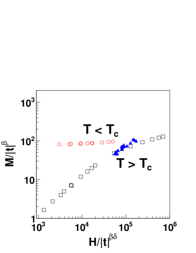
Figure 11: Scaling form for magnetization M vs. external field for nickel huang , open symbols. The corresponding quantities for nuclei normalized to the metal case are given by the full symbols.

Once we have derived the ‘reduced’ parameters of the Landau $O(m^{6})$ theory, we can write a ‘reduced’ free energy as ($b\neq 0$):

$$\frac{f}{T}=\frac{1}{2}xm^{2}-|z|m^{4}+\frac{2}{3}z^{2}m^{6}-\frac{{\it h}}{T}m,$$ (13)

where: $\frac{f}{T}=\frac{4c}{b^{2}}\frac{F}{T}$, $z=\frac{c}{|b|}$, $\frac{h}{T}=\frac{4c}{b^{2}}\frac{H}{T}$. These quantities together with the temperature, Eq.(7), and the reduced order parameter y,of Eq.(8), constitute the Landau $O(m^{6})$ theory in dimensionless form. It is instructive to study how these quantities change with the reaction system as we did in figures (7) and (8).

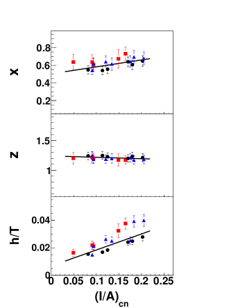
Figure 12: The parameters x, z and h/T versus (I/A) of the compound nucleus obtained from the data fit to the Landau free energy, Eq.(3). The symbols are like in figure 6.

In Fig.(12) we plot these normalized quantities vs. difference in neutron proton concentration of the compound nucleus. Compare to figure 7. A feature worth noticing is the following, while the parameter $a$ is decreasing with increasing (I/A) of the compound nucleus, the opposite holds for the parameter $x$ which gives the ‘distance’ from the critical temperature, see Fig.(12). This is very important since only normalized quantities should be used when inferring the properties of the EOS (i.e. temperature, density etc.) near the critical point.

IV Symmetry and Pairing compared to the Coulomb Energy.

In the previous sections we have seen that the Coulomb energy might become important especially for large values of the charges. We can now try to derive some qualitative understanding of when and why Coulomb corrections might become important and might even hinder a possible phase transition. From the mass formula we can write the Coulomb energy for large Z as pres :

$$\frac{E_{c}}{A}=0.77\frac{Z^{2}}{A^{2}}A^{2/3}=\frac{0.77}{4}(1-m)^{2}A^{2/3},$$ (14)

which explicitly introduces the order parameter $m$ in the Coulomb energy. We can define an ‘effective’ symmetry energy (per particle) as:

$$\frac{E_{eff}}{A}=(a_{sym}+\frac{0.77}{4}A^{2/3})m^{2}-\frac{0.77}{2}A^{2/3}m+\frac{0.77}{4}A^{2/3},$$ (15)

where the symmetry energy coefficient $a_{sym}=25MeV$. Ignoring for a moment density corrections we see that $O(m^{2})$ term should be affected by Coulomb corrections for large fragment mass numbers. Furthermore, a linear term in $m$ is introduced which will then modify the ‘external’ field even in collisions where the source $m_{s}=0$ as we discussed in Fig.(6). Finally there is a term not dependent on $m$ that will destroy the scaling for large mass (charge) numbers. We should also notice that assuming a spherical expansion, at low densities the Coulomb energy will decrease as $\rho^{1/3}$ while contributions to the symmetry energy should depend both on $\rho^{2/3}$ reflecting the Fermi energy of the nuclei and on $\rho$, the latter coming from different n-p interactions. At low densities we would expect Coulomb to be stronger than it appears to be in the data. This may be indicative that the fragments must be highly deformed, reducing the Coulomb energy. Coulomb corrections should become more important when $m=0$ for the detected fragment. We have plotted the yields of $m=0$ nuclei in Fig.(2) and pointed out that pairing appears to be playing a role. From Eq.(15) above we should expect that, if Coulomb is dominant for such fragments, the free energy should depend on $A^{2/3}$. In Fig.(13) (top panel) we plot F/T versus $A$ for $m=0$ fragments. The expected dependence with mass number in the free energy suggested from ‘effective’ symmetry energy Eq.(15) is not seen in the figure.

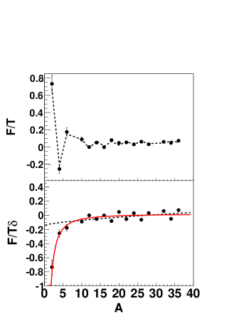
Figure 13: Free energy versus mass for $m=0$ isotopes for the ⁷⁰Zn+¹²⁴Sn system (top panel), the dashed line is a fit using Coulomb and pairing contributions. Free energy times $\delta$ (see text-bottom panel) versus mass for $m=0$ isotopes. The lines are separate fits suggested by the Coulomb(dashed line) and pairing(full line) energy mass number dependence.

Rather, a staggering between odd-odd and even-even nuclei is clearly visible.

To better clarify these arguments we can write the pairing energy from the mass formula as pres :

$$\frac{E_{p}}{A}=12\frac{\delta}{A^{3/2}},$$ (16)

where $12MeV$ is the ground state pairing energy coefficient and $\delta$:

$$\delta=\frac{(-1)^{N}+(-1)^{Z}}{2}.$$ (17)

The suggested mass dependence from pairing, Eq.16, is completely different from the Coulomb one when $m=0$, see Eq.14.

Notice that it is the $\delta$ factor from pairing that changes the sign of the contribution for odd-odd to even-even nuclei. A combined fit to the data using Coulomb plus pairing contributions results in the dashed line in Fig.(13), top panel. The agreement with data is very good. If we multiply the pairing energy by the factor $\delta$ we should get no discontinuities when plotting this quantity versus mass number. Similarly if the properties of the free energy depend on the pairing term, as for the ground state case, then it should be a monotonic function of $A$ after multiplying it by $\delta$. In Fig.(13) (bottom panel), we plot the quantity $\frac{F}{T}\delta$ versus mass number for the same system of Fig.(13) (top panel). The fit using the pairing mass dependence is also good. The Coulomb mass dependence fails especially for small mass number. From the values of the fit, using the ground state coefficients we can derive a temperature for the Coulomb case of $T=9.2(\frac{\rho}{\rho_{0}})^{1/3}MeV$ where we have explicitly indicated a possible density correction. For the pairing case we get $T=6.45MeV$. Notice that in this case we have not suggested any density correction since the fate of the pairing energy at low density and finite temperature is ‘terra incognita’. When making a combined fit using pairing and Coulomb energy we get a good reproduction of the data (dashed line in Fig.(13),top panel). While the fitting value for pairing results in a ‘temperature’ T=5.13 MeV, we get an increase of the Coulomb contribution to T=12.1 MeV. Assuming that pairing is independent on density, we could derive a density from the Coulomb result. A simple calculation give $\frac{\rho}{\rho_{0}}=(6.45/9)^{3}=0.34$ which could be a reasonable indication of the density of the system when it breaks into fragments.

In summary in this section we have shown that the role of the Coulomb energy appears to be rather reduced in the reactions analyzed in this paper. We expect it to become more important for large nuclei. On the other hand large nuclei have smaller symmetry and pairing energies per nucleon, thus a precise determination of the EOS can be obtained from measurements of isotopes having relatively small masses.

V dynamics of the phase transition

As we have seen we have been able to discuss some observables in the fragmentation of nuclei using a language common to macroscopic systems undergoing a phase transition. In the nuclear case we have a finite system composed at most of hundreds of particles which evolves in time under the influence of a long range Coulomb force. This poses many questions on why techniques of statistical mechanics should apply in such evolving nuclear systems. This also offers the possibility of dealing with statistical mechanics of open systems and the problem of extending the description of a phase transition to such a system.

We start by observing that even though we are dealing with a dynamical system, the order parameter defined in this work, $m$, is confined between -1 and +1. In this sense we have a somewhat ‘closed’ system. Also the density at which the transition occurs should be smaller then normal density and thus Coulomb effects are reduced. However, if we deal with larger sources, such as in U+U collisions the phase transition might be washed out by the strong Coulomb field. We expect our current considerations to be valid for small sources only.

From statistical mechanics we know that in a first order phase transition huang a small seed increases in size depending upon the surface tension at a given T and density $\rho$. If the pressure of the surrounding matter is smaller than the internal pressure of the drop, the drop will grow by capturing surrounding matter. On the other hand if the opposite is true then the drop will decrease in size to balance the external pressure. The entire process is driven by surface tension. Drops of a given size will survive only when their internal pressure balances the external pressure. If the system is at a very low density the interaction between different parts might take a relatively long time. In these conditions a big nuclear drop whose internal pressure is larger than that of the surroundings could be considered to be a nucleus which is evaporating particles in order to balance the external (zero in the case of an isolated nucleus) pressure. If we accept this picture than the evaporation step is part of the dynamics of the phase transition. Thus a very low density system might be thought of as many isolated drops evaporating particles and reaching their equilibrium conditions before they collide with other parts of the system or as small fragments being evaporated by other drops. In a finite system this does not happen, but we might think of a process where at some point the finite system becomes unconfined and an infinite system is approximated by an infinite number of repetitions or ‘events’. Of course in a statistically equilibrated system we know that time averages and event averages are the same. Here we are extending this concept to finite systems where only event averages can be used. A major question here is whether the properties of the phase transition are decided very early, i.e. when the system ‘enters’ the instability region. As we said above if we have an infinite system at a very low density undergoing a first order phase transition, then the drops can explode, evaporate, and fuse with other particles over a very long time. Our finite system might behave similarly but without the fusion at later times. If this were the case than the detected fragments carry all the information of the phase transition, if not then we need to reconstruct the primary fragment distributions coming out of the instability region.

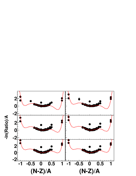
Figure 14: Free energy vs. time in AMD calculations (see text) for ⁶⁴Zn+¹¹²Sn system at 40MeV/A and central collisions, i.e. impact parameter less than 3 fm. Different picture correspond to T=200, 300, 500, 1000, 1500 and 2000 fm/c respectively.

We can try to clarify some of these questions by means of microscopic models such as Antisymmetrized Molecular Dynamics (AMD) or similar approaches where the time evolution of the system is followed ono . However, we have to stress that in such microscopic models some assumptions are made in order to recognize the fragments at particular times during the time evolution. In simpler approaches, fragments are recognized if particles are close in coordinate space (of the order of the range of the attractive nuclear forces) bon00 . In such a case the recognized fragments are ‘excited’ and they evolve in time until a final state is reached after a long time of the order of thousands of fm/c. A more refined approach for fragment recognitions is given by defining clusters when its components are within a given distance in phase space. The naive expectation would be that in this case we should recognize fragments earlier than the previous case and this is the method that we will adopt here for simplicity following ref. ono . In an ambitious approach dorso the claim is that fragments are recognized very early during the time evolution, of the order of tens of fm/c, if one searches for particles connected in phase space to form fragments and minimize the energy. This case probably corresponds to minimizing the entropy of the fragmenting system. If this last picture will hold true then a picture of an infinite system at low density will be equivalent to an ‘infinite’ repetition of events. Finally in all the considerations above we have to add the necessary and interesting complication that we have a mixture and not a single fluid, thus we can have more situations to explore than discussed in the previous sections and we can ‘turn on and off’ an external field as well.

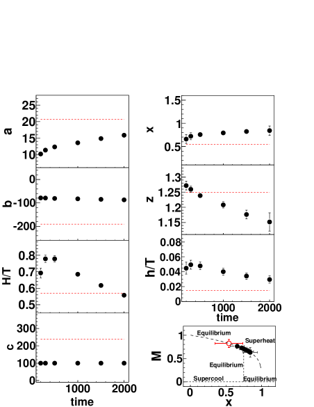
Figure 15: Fit parameters a, b and c vs. time (see text) for the same system of Fig.14. Solid circles refer to AMD calculations while the open symbol in the M vs. x plot is the experimental value for this system.

We have performed AMD calculations for the same systems investigated experimentally. After some time t, fragments are separated enough in phase space that we can recognize within a simple phase space coalescence approach as discussed in ono . In this way we can define a yield at a given time and from this derive the free energy exactly as we did with the experimental data. Characteristic results for the free energy versus time is given in Fig.(14) together with a Landau $O(m^{6})$ fit. Some time evolution is observed. Using a more sophisticated fragment recognition approach dorso might even decrease the time over which this evolution occurs. We can study the time evolution in more detail by plotting the variables a, b and c. M defined in the previous sections versus time. The results of the fits to the free energy at different times is given in Fig.(15). While the quantities a, b and H/T change somewhat during the time evolution, smaller changes are observed in the time evolution of normalized quantities, x, z and h/T. Nevertheless the time evolution of the fitting parameters influences the time evolution of the order parameter M versus reduced temperature x as seen in the bottom right of Fig.(15). It is very interesting to see that in these units the system is initially very hot (superheated) and cools down when coming to equilibrium below the critical temperature. The final result is very close to the observed values given by the open points.

Thus in this model most qualitative features of the phase transition are decided very early during the time evolution. This might correspond to an entropy saturation early during the evolution. However, different models and fragment recognition approaches might change the picture somewhat.

VI Equation of state

Once we know the free energy (at least in some cases) we can calculate the NEOS by means of the Fisher model fisher . Since we do not have at present experimental information on the density $\rho$, temperature T and pressure P of the system we can only estimate the ‘reduced pressure’ paolo :

$$\frac{P}{\rho T}(m)=\frac{M_{0}}{M_{1}},$$ (18)

where $M_{i}$ are moments of the mass distribution given by:

$$M_{k}=\sum_{A}A^{k}Y(A,m)=Y_{0}\sum_{A}A^{k}A^{-\tau}e^{-F/T(m)A};$$

$$k=0,...n.$$ (19)

Notice that the quantities above are now dependent on the order parameter m. From the knowledge of $F/T$ $(H/T=0)$ from the previous section we can easily calculate the reduced pressure near the critical point. In particular given the simple expression for the moments we can also derive some analytical formulas following paolo :

$$\frac{P}{\rho T}(m)=\frac{3.072|F/T|^{4/3}+1.417-3.631|F/T|+...}{-4.086|F/T|^{1/3}+3.631+0.966|F/T|+...},$$ (20)

which gives at the critical point a critical compressibility factor ($F/T=0$): $\frac{P}{\rho T}|_{c}=\frac{1.417}{3.631}=0.39$.
This value is essentially that derived from the Van-der-Waals gas equation but is well above the values observed for real gases. Using the relations above we can calculate the NEOS for the situations illustrated in Fig.9. The results are displayed in Fig.16 where the reduced pressure is plotted versus m for vaporization, superheating and first order phase transitions on the tri-critical line. Notice that there is not a large difference between the first two cases, while the last case displays two critical points (a third one is on the negative m axis).
We have seen in Fig.2 that $N=Z$ nuclei display a power law. We can also estimate the critical reduced pressure for this case noticing that the sums in Eq.(VI) above must be restricted to $A=2Z$ nuclei. This leads to a critical compressibility factor $\frac{P}{\rho T}_{c}=0.20$ which is a value closer to that estimated from other multi-fragmentation studies before mor .

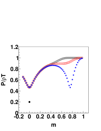
Figure 16: Reduced pressure versus m of the fragments obtained from the a, b and c parameters fit to the Landau free energy, Eq.(3) for the ⁶⁴Ni+²³²Th. The curves correspond to vapor(open circles), superheating(open squares), first order (3 critical line-solid stars), see text. The solid circle is for $N=Z$ nuclei at the critical point.

We can compare our analytical result given in Eq.(20) with the numerical values obtained above. This is displayed in Fig.(17) and we see that the numerical approximation is especially good near the critical point(s) as expected. If, from detailed comparison to experimental data, we are able to extract the temperature and pressure dependence of the parameters entering the Landau free energy, then Eq.(18) would be the Nuclear equation of state near a critical point. From the actual data at our disposal we can only estimate the behavior of the reduced pressure as function of the order parameter m.

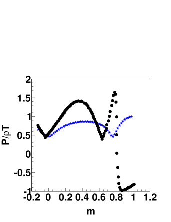
Figure 17: Comparison to the analytical result, Eq.(20)(solid circles) for a first order phase transition.

On similar ground we can define a reduced compressibility as

$$\chi\rho T(m)=\frac{M_{2}}{M_{1}}.$$ (21)

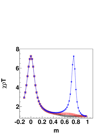
Figure 18: Reduced compressibility versus m of the fragments as in Fig.(16)

Its behavior is displayed in Fig.(18) for the cases outlined above. Divergences near the critical point(s) are obtained.

VII conclusions

In conclusion, in this paper we have presented and discussed experimental evidence for the observation of a quantum phase transition in nuclei, driven by the neutron/proton asymmetry. Using the Landau approach, we have derived the free energies for our systems and found that they are consistent with the existence of a line of first-order phase transitions terminating at a point where the system undergoes a second-order transition. The properties of the critical point depend on the symmetry. This is analogous to the well known superfluid $\lambda$ transition in ³He-⁴He mixtures. We suggest that a tricritical point, observed in ³He-⁴He systems may also be observable in fragmenting nuclei. These features call for further vigorous experimental investigation using high performance detector systems with excellent isotopic identification capabilities. Extension of these investigations to much larger asymmetries should be feasible as more exotic radioactive beams become available in the appropriate energy range.

It is important to stress that the observables discussed here represents only $necessary$ conditions for a critical behavior. A definite proof of a phase transition and a tricritical point could be given by a precise determination of yields of fragments whose $m\approx\pm 0.5$, i.e. very unstable nuclei which, most probably, decay before reaching the detectors. Thus fragment-particle correlation measurements for exotic primary fragments such as ${}^{4}Li$, ${}^{5}Be$ (proton rich) or extremely neutron rich ${}^{10}He$ are needed. More generally, such correlation experiments can also shed light on the effects of secondary decay on the fragment observables. This remains a key question in many equation of state studies and model calculations differ in their assessment of these effects wci ; bon00 . Higher quality data over a wider range of beam energies and colliding systems should also help in clarifying the role of other energy terms, such as surface, Coulomb etc., which are important at lower excitation energies. In particular the role of pairing and the possibility of Bose-Einstein condensation, should be more deeply investigated. Our data for $I=0$ fragments already show that pairing is important. This might be due to its importance during the phase transition or to its role during secondary decay of the excited primary fragments. Exploration of quantum phase transitions in nuclei is important to our understanding of the nuclear equation of state and can have a significant impact in nuclear astrophysics, helping to clarify the evolution of massive stars, supernovae explosions and neutron star formation.

- (1) M. A. Preston, Physics of the nucleus, Addison-Wesley pub., Reading-Mass. (1962).
- (2) K. Huang, Statistical Mechanics, second edition, ch.16-17, J. Wiley and Sons, New York, 1987.
- (3) L. D. Landau, E. M. Lifshitz, Statistical Physics, 3rd edition, Pergamon press, New York,1989.
- (4) A.Bonasera et al., Phys. Rev. Lett. 101, 122702 (2008).
- (5) M. Huang et al.,arXiv:1002.0311 [nucl-ex]
- (6) WCI proceedings, Ph. Chomaz et al., eds., EPJ A30 (2006), numb.1.
- (7) A. Bonasera et al., Rivista Nuovo Cimento, 23 (2000) 1.
- (8) H. Muller and B. D. Serot, Phys. Rev. C52 (1995) 2072; P.J. Siemens and G. Bertsch, Phys. Lett. B126 (1983) 9; P. J. Siemens, Nature 336 (1988) 109.
- (9) M. Belkacem, V. Latora, and A. Bonasera, Phys. Rev.C52 (1995) 271; A. Bonasera et al., Phys. Lett. B244 (1990) 169.
- (10) C. O. Dorso, V. C. Latora, and A. Bonasera, Phys. Rev. C60 (1999) 034606; M. Belkacem et al., Phys Rev. C54 (1996) 2435.
- (11) J. B. Elliott et al., Phys. Rev. Lett. 88 (2002) 042701; L. G. Moretto et al., Phys. Rev. Lett. 94 (2005) 202701.
- (12) M. D’Agostino et al., Nucl. Phys. A650 (1999) 329.
- (13) P. F. Mastinu et al., Phys. Rev. Lett. 76 (1996) 2646.
- (14) K. Hagel et al., Phys. Rev. C62 (2000) 034607.
- (15) J. Pochodzalla et al., Phys. Rev. Lett. 75 (1995) 1040.
- (16) V.Baran et al., Phys.Rep.410(2005)335.
- (17) M. Huang et al.,arXiv:1001.3621 [nucl-ex]
- (18) Z.Chen et al.,arXiv:1002.0319 [nucl-ex]
- (19) R.W. Minich et al., Phys.Lett.B118(1982)458.
- (20) N. Marie et al., Phys. Rev. C58 256 (1998).
- (21) M. E. Fisher, Rep. Prog. Phys. 30 (1967) 615.
- (22) A. Ono and H. Horiuchi, Progr. Part. Nucl. Phys. 53 (1996) 2958; A. Ono, Phys. Rev. C59 (1999) 853.
- (23) X. Campi, H. Krivine and N. Sator, Nucl. Phys. A681 (2001)458.
- (24) F. Gulminelli, Ph. Chomaz, M. Bruno, and M. D Agostino, Phys. Rev.C65 051601(R) (2002).
- (25) P. Finocchiaro et al. Nucl.Phys.A600(1996)236; T.Kubo et al. Zeit.Phys.A352(1995)145.