Asteroseismological Analysis of Rich Pulsating White Dwarfs

Abstract

We present the results of the asteroseismological analysis of two rich DAVs, G38-29 and R808, recent targets of the Whole Earth Telescope. 20 periods between 413 s and 1089 s were found in G38-29’s pulsation spectrum, while R808 is an even richer pulsator, with 24 periods between 404 s and 1144 s. Traditionally, DAVs that have been analyzed asteroseismologically have had less than half a dozen modes. Such a large number of modes presents a special challenge to white dwarf asteroseismology, but at the same time has the potential to yield a detailed picture of the interior chemical make-up of DAVs. We explore this possibility by varying the core profiles as well as the layer masses. We use an iterative grid search approach to find best fit models for G38-29 and R808 and comment on some of the intricacies of fine grid searches in white dwarf asteroseismology.

1 Astrophysical context

G38-29 and R808 are high amplitude, cool hydrogen dominated atmosphere pulsating white dwarfs (cDAVs). cDAVs are of interest for studying convection using the shape of their highly non-linear light curves (Montgomery, 2007). In addition, G38-29 and R808 are rich white dwarf pulsators, with over 20 periods present in their power spectrum. This makes them ideal subjects for asteroseismological studies. With the exception of hot pulsating white dwarfs (e.g. Córsico et al., 2006) , such rich pulsating white dwarfs have not been analyzed asteroseismologically before. Because of the large number of periods, asteroseismological identification of the modes in these stars is necessary in order to keep the study of convection using non-linear light curve fitting techniques computationally tractable.

With such a large number of modes, we can begin to probe the interior structure of white dwarfs in more detail. Cool pulsating white dwarfs have the advantage of being simpler to model than hot white dwarfs. The chemical elements in their interiors are nearly fully settled and much of their interiors close to fully degenerate. In addition, there are over 100 known DAVs (Castanheira et al., 2006) as opposed to 5 known DOVs (Quirion et al., 2007). Not all DAVs are rich pulsators, but with improved observational techniques, there is a potential to increase the number of modes observed in these stars, providing useful data for detailed asteroseismological analyses of white dwarf interiors.

In this paper, we present preliminary asteroseismological analyses of G38-29 and R808, based on Whole Earth Telescope (WET) campaigns performed in fall 2007 and spring 2008 (Thompson et al., 2009). We are able to derive stellar parameters such as mass and effective temperature for each star as well as internal structure parameters. We suggest an identification for the modes in each star.

2 Spectroscopy and Power Spectra

According to spectroscopy (Beauchamp et al., 1999), G38-29 has a temperature of 11,180 K and a $\log\rm g$ of 7.91, which translates to a mass of 0.55 $\rm M_{\odot}$. It was the object of a small WET campaign in November 2007. Analysis of the data revealed 20 independent modes, with periods ranging between 413.307 s and 1089.39 s. Of special interest in the power spectrum is an $\ell=1$ triplet, identified as such from average period spacing arguments. The triplet is split by 7 $\mu$Hz, leading to a rotational period of 21 hrs for the star and providing ground for the identification of additional multiplets (see Table 2). Out of the 20 independent modes, 15 are candidate m=0 modes.

R808 is similar in temperature to G38-29 (11,160 K), but more massive with a $\log\rm g$ of 8.04, corresponding to a mass of 0.63 $\rm M_{\odot}$. It was the object of a WET campaign in April 2008, where 25 independent modes were found in its somewhat noisier period spectrum. We tentatively identified 4 $\ell=2$ multiplets and 1 $\ell=1$ multiplet (see Table 2), consistent with a rotation period of 18 hours. The rotational splitting analysis leaves 18 possible m=0 modes.

3 Asteroseismological analysis

The periods observed in white dwarfs are g-modes, where the restoring force is buoyancy. In a completely homogeneous star, g-modes would be evenly spaced in period. In reality, white dwarfs are differentiated and the chemical transition zones induce a departure of the modes from their even spacings. The amount by which the modes deviate from their even spacing provides clues to the interior chemical structure of white dwarfs. In the presence of rotation, the modes get evenly split in frequency. The magnitude of the frequency split depends both on the rotational period and on the $\ell$ identification of the mode (Unno et al., 1989).

A rotational frequency splitting of 7 $\mu$Hz  corresponds to a $\Delta m=1$ period split of 1 second for a 400 s mode and 8 seconds for a 1100 s mode. For $\ell$=2 modes, the corresponding frequency split is near 11 $\mu$Hz, corresponding to 2 and 13 seconds split in periods for the 400 s and 1100 s modes respectively. These values are to compare with an average period spacing of $\sim$42 s for $\ell$=1 modes and $\sim$27 s for $\ell$=2 modes. For asteroseismological fits, this means that lower radial overtone modes (lower k) are less sensitive to the exact m identification than higher k modes. Fitting lower k modes first therefore minimizes modeling uncertainties due to our lack of knowledge of what the m identification of the modes is. On the other hand, lower k modes are also more sensitive to core structure in the model and magnify our a priori ignorance of the core chemical profiles. As a first pass, we assumed that the observed modes were m=0 modes and looked for an asymptotic period spacing in the observed period spectra of G38-29 and R808.

For our asteroseismological fits, we used the White Dwarf Evolution code (WDEC) to generate white dwarf models. The WDEC is described in detail in Lamb and van Horn (1975) and Wood (1990), and more recent modifications in Bischoff-Kim et al. (2007). We used an iterative grid search method varying 6 parameters, listed in Table 1, starting with a low resolution grid covering a wide region of parameter space in a range of effective temperature and mass suggested by the spectroscopic values. The grid is presented in Table 1. Based on the fits found, we successively refined the grid, focusing on the regions of parameter space where the best fit models resided at each iteration. The final grids have a resolution of 50 K in effective temperature, 0.002 $\rm M_{\odot}$  in mass for G38-29, and 0.005 $\rm M_{\odot}$  for R808, 0.002 (in the log) for the helium and hydrogen layer masses, 0.02 in central oxygen abundance and 0.02 $M_{*}$ for $X_{fm}$, the point where the oxygen abundance first starts to drop down.

Table 1: Parameters for the starting grid

Description	Parameter	Range	Step size
Effective temperature	$T_{\rm eff}$	10,600 -11,800 K	200 K
Stellar mass	$\rm M_{*}$	0.500 - 0.700 $\rm M_{\odot}$	0.010 $\rm M_{\odot}$
Helium layer mass	$\rm M_{He}$	$10^{-2.00}$ - $10^{-2.40}$	0.20 in the log
Hydrogen layer mass	$\rm M_{H}$	down to $10^{-7.00}$	0.20 in the log
Central oxygen abundance	$\rm X_{o}$	0.00 - 1.00	0.10
Point where oxygen abundance
first drops to zero	$\rm q_{fm}$	0.10 -0.80	0.10

4 Results

The results of the fits for G38-29 and R808 are presented in Table 2. For G38-29, the best fit model has a temperature of 11,550 K, a mass of 0.642 $\rm M_{\odot}$, a helium layer mass of $10^{-2.12}$, a hydrogen layer mass of $10^{-4.16}$. The central oxygen abundance is 0.80 and it starts dropping at mass point 0.68 $M_{*}$. For R808, the corresponding parameters are 11,250 K, 0.675 $\rm M_{\odot}$, $10^{-2.58}$, $10^{-4.62}$, $\rm X_{o}$= 0.10, and $X_{fm}=0.84$.

Table 2: Mode identification and best fit model periods for G38-29 and R808

G38-29					R808
Observed	Model	$\ell$	k	m	Observed	Model	$\ell$	k	m
Period	Period				Period	Period
432	428	1	7	0	405	406	1	6	0
545		1	10	+1	745	741	1	14	0
547	545	1	10	0	875	870	1	17	0
549		1	10	-1	912	912	1	18	0
706	705	1	14	0	915		1	18	-1
709		1	14	-1
962	957	1	20	0	952	954	1	19	0
1002	1002	1	21	0	1040	1042	1	21	0
1082		1	23	0
1089	1086	1	23	+1
413	409	2	14	0	511	514	2	17	0
					629		2	22	+1
					632	637	2	22	0
					796	788	2	28	0
					843	837	2	30	0
					860	862	2	31	0
840	844	2	32	0	878		2	32	+1
					899		2	32	-2
					908		2	33	+1
					916	914	2	33	0
					923		2	33	-1
900	900	2	34	0	952		2	35	+1
923	927	2	35	0	961	965	2	35	0
945	940	2	36	0
964	963	2	37	0	1011	1016	2	37	0
980		2	38	+1
990	992	2	38	0	1042	1042	2	38	0
1016	1022	2	39	0	1067	1067	2	39	0
					1091	1092	2	40	0
1087	1087	2	42	0	1144	1144	2	42	0

The quality of each period fit for G38-29 is illustrated in Figure 1. For $\ell=1$ modes, the uncertain m identifications can lead to uncertainties in model parameters, but not in $\ell$ and k identification. For $\ell=2$ modes, the situation becomes more ambiguous for higher k modes, as the frequency splitting translates to a period splitting that is of the same order as the average period spacing. Consecutive multiplets start to overlap.

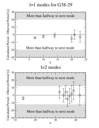
Figure 1: Quality of fit for the G38-29. The “error bars” are not error bars, but indicate the extent of the $\Delta m=\pm 1$ rotational period splitting mentioned in the text. Note that this splitting is significantly less than the period spacing for $\ell=1$ modes, though they can lead to significant uncertainties in the model periods and parameters if misidentified in m value. For the $\ell=2$ modes, the frequency splitting translates to a period splitting that is of the same order as the average period spacing. The situation is aggravated by the fact that $m=\pm 2$ modes are allowed as well.

5 Discussion

In grid searches, the question often arises “how fine is fine enough?”. How finely do we need to sample parameter space in order to find any minimum present? Sampling tests are needed to fully answer that question, though we can check that our solution approaches the minimum monotonically. The step sizes for the final, high resolution grid quoted in the previous section appear sufficiently small. This also means that if one wanted to create a grid that covers the parameter ranges listed in Table 1, one would have to calculate $\sim 10^{10}$ models. This is not manageable and the recourse is either to use “smarter” search algorithms such as genetic algorithms (Metcalfe and Charbonneau, 2003) or successively zooming in on the best fit. The two methods are complementary to each other. Genetic algorithms, given enough modes, are effective at finding a global minimum while grid searches help refining the minimum and provide more flexibility in trying different mode identifications.

The results presented here are preliminary, as we have made the assumption that all observed modes that were not members of multiplets were m=0 modes. As noted earlier, this assumption does not significantly influence the fits for k$\leq$10 modes, but becomes important for higher k modes. Observationally, m=0 modes are not necessarily the higher amplitude modes in multiplets suggesting that single modes may not be m=0 modes. Lightcurve fitting techniques provide an independent way of mode identification (Montgomery, 2008). It would be worth trying more general fits and using light curve fitting techniques for G38-29, where the observed frequencies are better determined.

References

- Montgomery (2007) M. H. Montgomery, “Using Non-Sinusoidal Light Curves of Multi-Periodic Pulsators to Constrain Convection,” in 15th European Workshop on White Dwarfs, edited by R. Napiwotzki, and M. R. Burleigh, 2007, vol. 372 of Astronomical Society of the Pacific Conference Series, pp. 635–+.
- Córsico et al. (2006) A. H. Córsico, L. G. Althaus, and M. M. Miller Bertolami, A&A 458, 259–267 (2006), arXiv:astro-ph/0607012.
- Castanheira et al. (2006) B. G. Castanheira, S. O. Kepler, F. Mullally, D. E. Winget, D. Koester, B. Voss, S. J. Kleinman, A. Nitta, D. J. Eisenstein, R. Napiwotzki, and D. Reimers, A&A 450, 227–231 (2006), arXiv:astro-ph/0511804.
- Quirion et al. (2007) P.-O. Quirion, G. Fontaine, and P. Brassard, ApJS 171, 219–248 (2007).
- Thompson et al. (2009) S. E. Thompson, J. L. Provencal, A. Kanaan, M. H. Montgomery, A. Bischoff-Kim, H. Shipman, and the WET team, “Whole Earth Telescope Observations of the DAVs R808 and G38-29,” Astronomical Society of the Pacific Conference Series, 2009.
- Beauchamp et al. (1999) A. Beauchamp, F. Wesemael, P. Bergeron, G. Fontaine, R. A. Saffer, J. Liebert, and P. Brassard, ApJ 516, 887–891 (1999).
- Unno et al. (1989) W. Unno, Y. Osaki, H. Ando, H. Saio, and H. Shibahashi, Nonradial oscillations of stars, 1989.
- Lamb and van Horn (1975) D. Q. Lamb, and H. M. van Horn, ApJ 200, 306–323 (1975).
- Wood (1990) M. A. Wood, Astero-archaeology: Reading the galactic history recorded in the white dwarf stars, Ph.D. thesis, AA(Texas Univ., Austin.) (1990).
- Bischoff-Kim et al. (2007) A. Bischoff-Kim, M. H. Montgomery, and D. E. Winget, ArXiv e-prints 7112039 (2007), 0711.2039.
- Metcalfe and Charbonneau (2003) T. S. Metcalfe, and P. Charbonneau, Journal of Computational Physics 185, 176–193 (2003), arXiv:astro-ph/0208315.
- Montgomery (2008) M. H. Montgomery, Communications in Asteroseismology 154, 38–48 (2008).