Quantum Diffusion and Eigenfunction Delocalization in a Random Band Matrix Model

Abstract

We consider Hermitian and symmetric random band matrices $H$ in $d\geqslant 1$ dimensions. The matrix elements $H_{xy}$, indexed by $x,y\in\Lambda\subset\mathbb{Z}^{d}$, are independent, uniformly distributed random variables if $\lvert x-y\rvert$ is less than the band width $W$, and zero otherwise. We prove that the time evolution of a quantum particle subject to the Hamiltonian $H$ is diffusive on time scales $t\ll W^{d/3}$. We also show that the localization length of the eigenvectors of $H$ is larger than a factor $W^{d/6}$ times the band width. All results are uniform in the size $\lvert\Lambda\rvert$ of the matrix.

AMS Subject Classification: 15B52, 82B44, 82C44

Keywords: Random band matrix, Anderson model, localization length

1 Introduction

The general formulation of the universality conjecture for disordered systems states that there are two distinctive regimes depending on the energy and the disorder strength. In the strong disorder regime, the eigenfunctions are localized and the local spectral statistics are Poisson. In the weak disorder regime, the eigenfunctions are delocalized and the local statistics coincide with those of a Gaussian matrix ensemble.

Random band matrices are natural intermediate models to study eigenvalue statistics and quantum propagation in disordered systems as they interpolate between Wigner matrices and random Schrödinger operators. Wigner matrix ensembles represent mean-field models without spatial structure, where the quantum transition rates between any two sites are i.i.d. random variables with zero expectation. In the celebrated Anderson model [5], only a random on-site potential $V$ is present in addition to a short range deterministic hopping (Laplacian) on a graph that is typically a regular box in $\mathbb{Z}^{d}$.

For the Anderson model, a fundamental open question is to establish the metal-insulator transition, i.e. to show that in $d\geqslant 3$ dimensions the eigenfunctions of $-\Delta+\lambda V$ are delocalized for small disorder $\lambda$. The localization regime at large disorder or near the spectral edges has been well understood by Fröhlich and Spencer with the multiscale technique [29, 30], and later by Aizenman and Molchanov by the fractional moment method [3]; many other works have since contributed to this field. In particular, it has been established that the local eigenvalue statistics are Poisson [38] and that the eigenfunctions are exponentially localized with an upper bound on the localization length that diverges as the energy parameter approaches the presumed phase transition point [43, 15].

The progress in the delocalization regime has been much slower. For the Bethe lattice, corresponding to the infinite-dimensional case, delocalization has been established in [35, 4, 27]. In finite dimensions only partial results are available. The existence of an absolutely continuous spectrum (i.e. extended states) has been shown for a rapidly decaying potential, corresponding to a scattering regime [39, 8, 10]. Diffusion has been established for a heavy quantum particle immersed in a phonon field in $d\geqslant 4$ dimensions [28]. For the original Anderson Hamiltonian with a small coupling constant $\lambda$, the eigenfunctions have a localization length of at least $\lambda^{-2}$ (see [9]). The time and space scale $\lambda^{-2}$ corresponds to the kinetic regime where the quantum evolution can be modelled by a linear Boltzmann equation [45, 24]. Beyond this time scale the dynamics is diffusive. This has been established in the scaling limit $\lambda\to 0$ up to time scales $t\sim\lambda^{-2-\kappa}$ with an explicit $\kappa>0$ in [18, 19, 20]. There are no rigorous results on the local spectral statistics of the Anderson model, but it is conjectured – and supported by numerous arguments in the physics literature, especially by supersymmetric methods (see [14]) – that the local correlation function of the eigenvalues of the finite volume Anderson model follows the GOE statistics in the thermodynamic limit.

Due to their mean-field character, Wigner matrices are simpler to study than the Anderson model and they are always in the delocalization regime. The complete delocalization of the eigenvectors was proved in [21]. The local spectral statistics in the bulk are universal, i.e. they follow the statistics of the corresponding Gaussian ensemble (GOE, GUE, GSE), depending on the symmetry type of the matrix (see [37] for explicit formulas). For an arbitrary single entry distribution, bulk universality has been proved recently in [17, 22, 23] for all symmetry classes. A different proof was given in [46] for the Hermitian case.

Random band matrices $H=\{H_{xy}\}_{x,y\in\Gamma}$ represent systems on a large finite graph $\Gamma$ with a metric. The matrix elements between two sites, $x$ and $y$, are independent random variables with a variance $\sigma_{xy}^{2}\mathrel{\mathop{:}}=\mathbb{E}|H_{xy}|^{2}$ depending on the distance between the two sites. The variance typically decays with the distance on a characteristic length scale $W$, called the band width of $H$. This terminology comes from the simplest one-dimensional model where the graph is a path on $N$ vertices, labelled by $\Gamma=\{1,2,\ldots,N\}$, and the matrix elements $H_{xy}$ vanish if $|x-y|\geqslant W$. If $W=N$ and all variances are equal, we recover the usual Wigner matrix. The case $W=O(1)$ is a one-dimensional Anderson-type model with random hoppings at bounded range. Higher-dimensional models are obtained if the graph $\Gamma$ is a box in $\mathbb{Z}^{d}$. For more general random band matrices and for a systematic presentation, see [44].

Since the one-dimensional Anderson-type models are always in the localization regime, varying the band width $W$ offers a possibility to test the localization-delocalization transition between an Anderson-type model and the Wigner ensemble. Numerical simulations and theoretical arguments based on supersymmetric methods [31] suggest that the local eigenvalue statistics change from Poisson, for $W\ll N^{1/2}$, to GOE (or GUE), for $W\gg N^{1/2}$. The eigenvectors are expected to have a localization length $\ell$ of order $W^{2}$. In particular the eigenvectors are fully delocalized for $W\gg N^{1/2}$. In two dimensions the localization length is expected to be exponentially large in $W$; see [1]. In accordance with the extended states conjecture for the Anderson model, the localization length is expected to be macroscopic, $\ell\sim N$, independently of the band width in $d\geqslant 3$ dimensions.

Extending the techniques of the rigorous proofs for Anderson localization, Schenker has recently proved the upper bound $\ell\leqslant W^{8}$ for the localization length in $d=1$ dimensions [40]. In this paper we prove a counterpart of this result from the side of delocalization. More precisely, we show a lower bound $\ell\geqslant W^{1+d/6}$ for the eigenvectors of $d$-dimensional band matrices with uniformly distributed entries. We remark that the lower bound $\ell\geqslant W$ was proved recently in [25] for very general band matrices.

On the spectral side, we mention that, apart from the semicircle law (see [2, 33, 25] for $d=1$ and [11] for $d=3$), the question of bulk universality of local spectral statistics for band matrices is mathematically open even for $d=1$. In the spirit of the general conjecture, one expects GUE/GOE statistics in the bulk for the delocalization regime, $W\gg N^{1/2}$. The GUE/GOE statistics have recently been established [25] for a class of generalized Wigner matrices, where the variances of different matrix elements are not necessarily identical, but are of comparable size, i.e. $\mathbb{E}|H_{xy}|^{2}\sim\mathbb{E}|H_{x^{\prime}y^{\prime}}|^{2}$; in particular, the band width is still macroscopic ($W\sim N$).

Supersymmetric methods offer a very attractive approach to study the delocalization transition in band matrices but the rigorous control of the functional integrals away from the saddle points is difficult and it has been performed only for the density of states [11]. Effective models that emerge near the saddle points can be more accessible to rigorous mathematics. Recently Disertori, Spencer and Zirnbauer studied a related statistical mechanics model that is expected to reflect the Anderson localization and delocalization transition for real symmetric band matrices. They proved a quasi-diffusive estimate for the two-point correlation functions in a three dimensional supersymmetric hyperbolic nonlinear sigma model at low temperatures [13]. Localization was also established in the same model at high temperatures [12].

We also mention that band matrices are not the only possible interpolating models to mimic the metal-insulator transition. Other examples include the Anderson model with a spatially decaying potential [8, 34] and a quasi one-dimensional model with a weak on-site potential for which a transition in the sense of local spectral statistics has been established in [6, 47].

A natural approach to study the delocalization regime is to show that the quantum time evolution is diffusive on large scales. We normalize the matrix entries so that the rate of quantum jumps is of order one. The typical distance of a single jump is the band width $W$. If the jumps were independent, the typical distance travelled in time $t$ would be $W\sqrt{t}$. Using the argument of [9], we show that a typical localization length $\ell$ is incompatible with a diffusion on spatial scales larger than $\ell$. Thus we obtain $\ell\geqslant W\sqrt{t}$, provided that the diffusion approximation can be justified up to time $t$.

The main result of this paper is that the quantum dynamics of the $d$-dimensional band matrix is given by a superposition of heat kernels up to time scales $t\ll W^{d/3}$. Although diffusion is expected to hold up to time $t\sim W^{2}$ for $d=1$ and up to any time for $d\geqslant 3$ (assuming the thermodynamic limit has been taken), our method can follow the quantum dynamics only up to $t\ll W^{d/3}$. The threshold exponent $d/3$ originates in technical estimates on certain Feynman graphs; going beyond the exponent $d/3$ would require a further resummation of certain four-legged subdiagrams (see Section 11).

Finally, we remark that our method also yields a bound on the largest eigenvalue of a band matrix; see Theorem 3.4 in the forthcoming paper [16] for details.

Acknowledgements

The problem of diffusion for random band matrices originated from several discussions with H.T. Yau and J. Yin. The authors are especially grateful to J. Yin for various insights and for pointing out an improvement in the counting of the skeleton diagrams.

2 The Setup

Let the dimension $d\geqslant 1$ be fixed and consider the $d$-dimensional lattice $\mathbb{Z}^{d}$ equipped with the Euclidean norm $\lvert\cdot\rvert_{\mathbb{Z}^{d}}$ (any other norm would also do). We index points of $\mathbb{Z}^{d}$ with $x,y,z,\dots$. Let $W>1$ denote a large parameter (the band width) and define

$$M\;\equiv\;M(W)\;\mathrel{\mathop{:}}=\;\big{\lvert}\{x\in\mathbb{Z}^{d}\,:\,1\leqslant\lvert x\rvert_{\mathbb{Z}^{d}}\leqslant W\}\big{\rvert}\,,$$

the number of points at distance at most $W$ from the origin. In the following we tacitly make use of the obvious relation $M\sim\;CW^{d}$. For notational convenience, we use both $W$ and $M$ in the following.

In order to avoid dealing with the infinite lattice directly, we restrict the problem to a finite periodic lattice $\Lambda_{N}$ of linear size $N$. More precisely, for $N\in\mathbb{N}$, we set

$$\Lambda_{N}\;\mathrel{\mathop{:}}=\;\{-[N/2],\dots,N-1-[N/2]\}^{d}\;\subset\;\mathbb{Z}^{d}\,,$$

a cube with side length $N$ centred around the origin. Here $[\cdot]$ denotes integer part. We regard $\Lambda_{N}$ as periodic, i.e. we equip it with periodic addition and the periodic distance

$$\lvert x\rvert\;\mathrel{\mathop{:}}=\;\inf\{\lvert x+N\nu\rvert_{\mathbb{Z}^{d}}\,:\,\nu\in\mathbb{Z}^{d}\}\,.$$

Unless otherwise stated, all summations $\sum_{x}$ are understood to mean $\sum_{x\in\Lambda_{N}}$.

We consider random matrices $H^{\omega}\equiv H$ whose entries $H_{xy}$ are indexed by $x,y\in\Lambda_{N}$. Here $\omega$ denotes the running element in probability space. The large parameter of the model is the band width $W$. We shall always assume that $N\geqslant WM^{1/6}$. Under this condition all our results hold uniformly in $N$.

We assume that $H$ is either Hermitian or symmetric. The entries $H_{xy}$ satisfying $1\leqslant\lvert x-y\rvert\leqslant W$ are i.i.d. (with the obvious restriction that $H_{yx}=\overline{H_{xy}}\!\,$). In the Hermitian case they are uniformly distributed on a circle of appropriate radius in the complex plane,

$$H_{xy}\;\sim\;\frac{1}{\sqrt{M-1}}\,\mathrm{Unif}(\mathbb{S}^{1})\,,\qquad 1\leqslant\lvert x-y\rvert\leqslant W\,.$$ (2.1a)

In the symmetric case they are Bernoulli random variables,

$$\mathbb{P}\biggl{(}{H_{xy}=\frac{1}{\sqrt{M-1}}}\biggr{)}\;=\;\mathbb{P}\biggl{(}{H_{xy}=\frac{-1}{\sqrt{M-1}}}\biggr{)}\;=\;\frac{1}{2}\,,\qquad 1\leqslant\lvert x-y\rvert\leqslant W\,.$$ (2.1b)

If $\lvert x-y\rvert\notin[1,W]$ then $H_{xy}=0$. An important consequence of our assumptions (2.1a) and (2.1b) is

$$\lvert H_{xy}\rvert^{2}\;=\;\frac{1}{M-1}\,\bm{\mathrm{1}}(1\leqslant\lvert x-y\rvert\leqslant W)\,.$$ (2.2)

We remark that the assumption that the matrix entries have the special form (2.1a) or (2.1b) is not necessary for our results to hold. We make it here because it greatly simplifies our proof. The reason for this is that, as observed by Feldheim and Sodin [26, 42], the condition (2.2) allows one to obtain a simple algebraic expression for the nonbacktracking powers of $H$; see Lemma 5.2.

In the forthcoming paper [16] we extend our results to random matrix ensembles in which the matrix elements $H_{xy}$ are allowed to have a general distribution (and thus in particular a genuinely random absolute value); moreover their variances $\mathbb{E}\lvert H_{xy}\rvert^{2}$ are given by a general profile on the scale $W$ in $x-y$ (as opposed to the step function profile in (2.2)). Under these assumptions, the algebraic identity of Lemma 5.2 is no longer exact, and needs to be amended with additional random terms. The resulting graphical expansion is considerably more involved than in the case (2.2), and its control requires essential new ideas. However, the fundamental mechanism underlying quantum diffusion for band matrices is already apparent in the special case (2.2) discussed in this paper.

Let $\alpha\in\mathfrak{A}\mathrel{\mathop{:}}=\{1,\dots,\lvert\Lambda_{N}\rvert\}$ index the orthonormal basis $\{\psi_{\alpha}^{\omega}\}_{\alpha\in\mathfrak{A}}$ of eigenvectors of the matrix $H^{\omega}$, i.e. $H^{\omega}\psi_{\alpha}^{\omega}=\lambda^{\omega}_{\alpha}\psi_{\alpha}^{\omega}$, where $\lambda_{\alpha}^{\omega}\in\mathbb{R}$. The normalization of the matrix elements is chosen in such a way that the typical eigenvalue of the matrix is of order one:

$$\frac{1}{\lvert\mathfrak{A}\rvert}\sum_{\alpha}\mathbb{E}\lambda_{\alpha}^{2}\;=\;\frac{1}{\lvert\mathfrak{A}\rvert}\mathbb{E}\operatorname{Tr}H^{2}\;=\;\frac{1}{\lvert\mathfrak{A}\rvert}\mathbb{E}\sum_{x,y}|H_{xy}|^{2}\;=\;\frac{M}{M-1}\,.$$

3 Scaling and results

The central quantity of our analysis is

$$\varrho(t,x)\;\mathrel{\mathop{:}}=\;\mathbb{E}\,\big{\lvert}\big{\langle}{\delta_{x}}\mspace{2.0mu},{\mathrm{e}^{-\mathrm{i}tH/2}\delta_{0}}\big{\rangle}\big{\rvert}^{2}\,,$$

where $\delta_{x}\in\ell^{2}(\Lambda_{N})$ denotes the standard basis vector, defined by $(\delta_{x})_{y}=\delta_{xy}$. The factor $1/2$ is a convenient normalization since, by a standard result of random matrix theory, the spectrum of $H/2$ is asymptotically equal to the unit interval $[-1,1]$. The function $\varrho(t,x)$ describes the ensemble average of the quantum transition probability of a particle starting from position $0$ ending up at position $x$ after time $t$. Note that $\sum_{x}\varrho(t,x)=1$ for any $t\in\mathbb{R}$. Heuristically, the particle performs a series of random jumps of size $W$. The typical number of jumps in time $t=O(1)$ is of order one. Indeed, by first order perturbation theory, the small-times probability distribution for $1\leqslant\lvert x\rvert\leqslant W$ is given by

$$\varrho(t,x)\;\sim\;\mathbb{E}\,\big{\lvert}\big{\langle}{\delta_{x}}\mspace{2.0mu},{(\mathbbmss{1}-\mathrm{i}tH/2)\delta_{0}}\big{\rangle}\big{\rvert}^{2}\;=\;\frac{t^{2}}{4}\,\mathbb{E}\,\lvert H_{x0}\rvert^{2}\;=\;\frac{t^{2}}{4}\,\frac{1}{M-1}\,,$$

up to higher order terms in $t$. Thus $\sum_{x\neq 0}\varrho(t,x)$ is an $O(1)$ quantity, separated away from zero, indicating that the distance from the origin is of $O(W)$ for times $t\sim O(1)$.

In time $t$ the particle performs $O(t)$ jumps of size $O(W)$. We expect that the jumps are approximately independent and the trajectory is a random walk consisting of $O(t)$ steps with size $O(W)$ each. Thus, the typical distance from the origin is of order $t^{1/2}W$. We rescale time and space $(t,x)\mapsto(T,X)$ so as to make the macroscopic quantities $T$ and $X$ of order one, i.e. we set

$$t\;=\;\eta T\,,\qquad x\;=\;\eta^{1/2}WX\,,$$

where $W$ and $\eta$ are two large parameters. Ideally, one would like to study the long time limit $\eta\to\infty$ for a fixed $W$. In this case, however, we know that the dynamics cannot be diffusive for $d=1$. Indeed, as explained in the introduction, it is expected that the motion cannot be diffusive for distances larger than $W^{2}$; this has in fact been proved [40] for distances larger than $W^{8}$. Thus we have to consider a scaling limit where $\eta$ and $W$ are related and they tend simultaneously to infinity. To that end we choose an exponent $\kappa>0$ and set $\eta\equiv\eta(W)\mathrel{\mathop{:}}=W^{d\kappa}$.

Our first main result establishes that $\varrho(t,x)$ behaves diffusively up to time scales $t=O(W^{d\kappa})$ if $\kappa<1/3$.

Theorem 3.1 (Quantum diffusion).

Let $0<\kappa<1/3$ be fixed. Then for any $T_{0}>0$ and any continuous bounded function $\varphi\in C_{b}(\mathbb{R}^{d})$ we have

$$\lim_{W\to\infty}\sum_{x\in\Lambda_{N}}\varrho\bigl{(}{W^{d\kappa}T,x}\bigr{)}\,\varphi\biggl{(}{\frac{x}{W^{1+d\kappa/2}}}\biggr{)}\;=\;\int_{\mathbb{R}^{d}}\mathrm{d}X\;L(T,X)\,\varphi(X)\,,$$ (3.1)

uniformly in $N\geqslant W^{1+d/6}$ and $0\leqslant T\leqslant T_{0}$. Here

$$L(T,X)\;\mathrel{\mathop{:}}=\;\int_{0}^{1}\mathrm{d}\lambda\;\frac{4}{\pi}\frac{\lambda^{2}}{\sqrt{1-\lambda^{2}}}\,G(\lambda T,X)\,,$$

and $G$ is the heat kernel

$$G(T,X)\;\mathrel{\mathop{:}}=\;\biggl{(}{\frac{d+2}{2\pi T}}\biggr{)}^{d/2}\,\mathrm{e}^{-\frac{d+2}{2T}\,\lvert X\rvert^{2}}\,,$$ (3.2)

Remark 3.2.

The factor $d+2$ arises from a random walk in $d$ dimensions with steps in the unit ball. If $B$ is a random variable uniformly distributed in the $d$-dimensional unit ball, the covariance matrix of $B$ is $(d+2)^{-1}\mathbbmss{1}$.

This result can be interpreted as follows. The limiting dynamics at macroscopic time $T$ is not given by a single heat kernel, but by a weighted superposition of heat kernels at times $\lambda T$, for $0\leqslant\lambda\leqslant 1$. The factor $\lambda$ expresses a delay arising from backtracking paths, in which the quantum particle “wastes time” by retracing its steps. If the particle is not backtracking, it is moving according to diffusive dynamics. The backtracking paths correspond to two-legged subdiagrams, and have the interpretation of a self-energy renormalization in the language of diagrammatic perturbation theory. Thus, out of the total macroscopic time $T$ during which the particle moves, a fraction $\lambda$ of $T$ is spent moving diffusively, and a fraction $(1-\lambda)$ of $T$ backtracking. Theorem 3.1 gives an explicit expression for the probability density $f(\lambda)=\frac{4}{\pi}\frac{\lambda^{2}}{\sqrt{1-\lambda^{2}}}\bm{\mathrm{1}}(0\leqslant\lambda\leqslant 1)$ for the particle to move during a fraction $\lambda$ of $T$.

Our proof precisely exhibits this phenomenon. As explained in Section 4, the proof is based on an expansion of the quantum time evolution in terms of nonbacktracking paths. At time $t=W^{d\kappa}T$, this expansion yields a weighted superposition of paths of lengths $n=1,\dots,[t]$ (higher values of $n$ are strongly suppressed). Here $n$ is the number of nonbacktracking steps, i.e. the number of steps that contribute to the effective motion of the particle. The difference $[t]-n$ is the number of steps that the particle spends backtracking. Our expansion (or, more precisely, its leading order ladder terms) shows that the weight of a path of $n$ nonbacktracking steps is given by $\lvert\alpha_{n}(t)\rvert^{2}$, where $\alpha_{n}(t)$ is the Chebyshev transform of the propagator $\mathrm{e}^{-\mathrm{i}t\xi}$ in $\xi$; see (5.3). The probability density $f$ arises from this microscopic picture by setting $n=[\lambda t]$. Then we have, as proved in Proposition 8.5 below, $t\lvert\alpha_{[\lambda t]}(t)\rvert^{2}\to f(\lambda)$ weakly as $t\to\infty$.

Our second main result shows that the eigenvectors of $H$ have a typical localization length larger than $W^{1+d\kappa/2}$, for any $\kappa<1/3$. For $x\in\Lambda_{N}$ and $\ell>0$ we define the characteristic function $P_{x,\ell}$ projecting onto the complement of an $\ell$-neighbourhood of $x$,

$$P_{x,\ell}(y)\;\mathrel{\mathop{:}}=\;\bm{\mathrm{1}}(\lvert y-x\rvert\geqslant\ell)\,.$$

Let $\varepsilon>0$ and define the random subset $\mathfrak{A}_{\varepsilon,\ell}^{\omega}\subset\mathfrak{A}$ of eigenvectors through

$$\mathfrak{A}^{\omega}_{\varepsilon,\ell}\;\mathrel{\mathop{:}}=\;\biggl{\{}{\alpha\in\mathfrak{A}\,:\,\sum_{x}\lvert\psi_{\alpha}^{\omega}(x)\rvert\,\lVert P_{x,\ell}\,\psi^{\omega}_{\alpha}\rVert<\varepsilon}\biggr{\}}\,.$$

The set $\mathfrak{A}^{\omega}_{\varepsilon,\ell}$ contains, in particular, all eigenvectors that are exponentially localized in balls of radius $O(\ell)$; see Corollary 3.4 below for a more general and precise statement.

Theorem 3.3 (Delocalization).

Let $\varepsilon>0$ and $0<\kappa<1/3$. Then

$$\limsup_{W\to\infty}\,\mathbb{E}\,\frac{\big{\lvert}\mathfrak{A}_{\varepsilon,W^{1+d\kappa/2}}\big{\rvert}}{\lvert\mathfrak{A}\rvert}\;\leqslant\;2\sqrt{\varepsilon}\,,$$

uniformly in $N\geqslant W^{1+d/6}$.

Theorem 3.3 implies that the fraction of eigenvectors subexponentially localized on scales $W^{1+\kappa d/2}$ converges to zero in probability.

Corollary 3.4.

For fixed $\gamma>0$ and $K>0$ define the random subset of eigenvectors

$$\mathfrak{B}^{\omega}_{\ell}\;\mathrel{\mathop{:}}=\;\biggl{\{}{\alpha\in\mathfrak{A}\,:\,\exists\,u\in\Lambda_{N}\,:\,\sum_{x}\lvert\psi_{\alpha}^{\omega}(x)\rvert^{2}\exp\biggl{[}{\frac{\lvert x-u\rvert}{\ell}}\biggr{]}^{\gamma}\leqslant K}\biggr{\}}\,.$$ (3.3)

Then for $0<\kappa<1/3$ we have

$$\lim_{W\to\infty}\mathbb{E}\,\frac{\lvert\mathfrak{B}_{W^{1+\kappa d/2}}\rvert}{\lvert\mathfrak{A}\rvert}\;=\;0\,,$$

uniformly in $N\geqslant W^{1+d/6}$.

4 Main ideas of the proof

We need to compute the expectation of the squared matrix elements of the unitary time evolution $\mathrm{e}^{-\mathrm{i}tH/2}$. A natural starting point is the power series expansion $\mathrm{e}^{-\mathrm{i}tH/2}=\sum_{n\geqslant 0}(-\mathrm{i}tH/2)^{n}/n!$. Unfortunately, the resulting series is unstable for $t\to\infty$, as is manifested by the large cancellations in the sum

$$\mathbb{E}\lvert\langle{\delta_{x}}\mspace{2.0mu},{\mathrm{e}^{-\mathrm{i}tH/2}\delta_{y}}\rangle\rvert^{2}=\sum_{n,n^{\prime}}\frac{\mathrm{i}^{n-n^{\prime}}t^{n+n^{\prime}}}{2^{n+n^{\prime}}n!n^{\prime}!}\,\mathbb{E}H^{n}_{xy}H^{n^{\prime}}_{yx}.$$ (4.1)

This can be seen as follows. The expectation

$$\mathbb{E}H^{n}_{xy}H^{n^{\prime}}_{yx}=\mathbb{E}\sum_{x_{1},\ldots x_{n-1}}\sum_{y_{1},\ldots y_{n^{\prime}-1}}H_{xx_{1}}H_{x_{1}x_{2}}\ldots H_{x_{n-1}y}H_{yy_{n^{\prime}-1}}\ldots H_{y_{1}x}$$ (4.2)

is traditionally represented graphically by drawing the labels $x,x_{1},x_{2},\dots,y_{1},x$ as vertices of a path, and by identifying vertices whose labels are identical. Since the matrix elements are centred (i.e. $\mathbb{E}H_{xy}$ = 0 for all $x,y$), each edge must be traveled at least twice in any path that yields a nonzero contribution to (4.2). It is well known that the leading order contribution to (4.2) is given by the so-called fully backtracking paths. A fully backtracking path is a path generated by successively applying the transformation $a\mapsto aba$ to the trivial path $x$. A typical fully backtracking path may be thought of as a tree with double edges. It is not hard to see that, after summing over $y$, each fully backtracking path yields a contribution of order 1 to (4.2). Also, the number of fully backtracking paths is of order $4^{n+n^{\prime}}$, so that the expectation (4.2) is of order $4^{n+n^{\prime}}$. In particular, this implies that the main contribution to (4.1) comes from terms satisfying $n+n^{\prime}\sim t$. Moreover, the series (4.1) is unstable in the sense that the sum of the absolute values of its summands behaves like $\mathrm{e}^{4t}$ as $t\to\infty$.

The large terms in (4.1) systematically cancel each other out similarly to the two-legged subdiagram renormalization in perturbative field theory. In perturbative renormalization, these cancellations are exploited by introducing appropriately adjusted fictitious counter-terms. In the current problem, however, we make use of the Chebyshev transformation, which removes the contribution of all backtracking paths in one step. The key observation is that, if $U_{n}$ denotes the $n$-th Chebyshev polynomial of the second kind, then $U_{n}(H/2)$ can be expressed in terms of nonbacktracking paths. A nonbacktracking path is a path which contains no subpath of the form $aba$. Thus the strongest instabilities in (4.1) can be removed if $\mathrm{e}^{-\mathrm{i}tH/2}$ is expanded into a series of Chebyshev polynomials. This idea appeared first in [7] and has recently been exploited in [26, 42] to prove, among other things, the edge-universality for band matrices. In [42] it is also stated that the same method can be used to prove delocalization of the edge eigenvectors if $W\geqslant N^{5/6}$, i.e. to get the bound $\ell\geqslant W^{6/5}$ on the localization length $\ell$. Our estimate gives a slightly weaker bound, $\ell\geqslant W^{7/6}$, for this special case, but it applies to bulk eigenvectors as well as higher dimensions.

After the Chebyshev transform, we need to compute expectations

$$\mathbb{E}\sideset{}{{}^{\prime}}{\sum}_{x_{1},\ldots x_{n-1}}\sideset{}{{}^{\prime}}{\sum}_{y_{1},\ldots y_{n^{\prime}-1}}H_{xx_{1}}H_{x_{1}x_{2}}\ldots H_{x_{n-1}y}H_{yy_{n^{\prime}-1}}\ldots H_{y_{1}x},$$ (4.3)

where the summations are restricted to nonbacktracking paths. As above, since $\mathbb{E}H_{ab}=0$ every matrix element must appear at least twice in the non-trivial terms of (4.3). Taking the expectation effectively introduces a pairing, or more generally a lumping, of the factors, which can be conveniently represented by Feynman diagrams. The main contribution comes from the so-called ladder diagrams, corresponding to $n=n^{\prime}$ and $x_{i}=y_{i}$. The contribution of these diagrams can be explicitly computed, and showed to behave diffusively. More precisely: Since we express nonbacktracking powers of $H$ as Chebyshev polynomials in $H/2$, the contribution of each graph to the propagator $\mathrm{e}^{-\mathrm{i}tH/2}$ carries a weight equal to the Chebyshev transform $\alpha_{n}(t)$ of $\mathrm{e}^{-\mathrm{i}t\xi}$ in $\xi$. We shall show that $\alpha_{n}(t)$ is given essentially by a Bessel function of the first kind. In order to identify the limiting behaviour of the ladder diagrams, we therefore need to analyse a probability distribution on $\mathbb{N}$ of the form $\bigl{\{}{\lvert\alpha_{n}(t)\rvert^{2}}\bigr{\}}_{n\in\mathbb{N}}$ for large $t$ (Section 8).

The main work consists of proving that the non-ladder diagrams are negligible. Similarly to the basic idea of [18, 19, 20], the non-ladder diagrams are classified according to their combinatorial complexity. The large number of complex diagrams is offset by their small value, expressed in terms of powers of $W$. Conversely, diagrams containing large pieces of ladder subdiagrams have a relatively large contribution but their number is small.

More precisely, focusing only on the pairing diagrams in the Hermitian case, it is easy to see that ladder subdiagrams are marginal for power counting. We define the skeleton of a graph by collapsing parallel ladder rungs (called bridges) into a single rung. We show that the value of a skeleton diagram is given by a negative power of $M\sim CW^{d}$ that is proportional to the size of the skeleton diagram. This is how the dimension $d$ enters our estimate. We then sum up all possible ladder subdiagrams corresponding to a given skeleton. Although the ladder subdiagrams do not yield additional $W$-powers, they represent classical random walks for which dispersive bounds are available, rendering them summable. The restriction $t\ll W^{d/3}$ comes from summing up the skeleton diagrams. In Section 11 we present a critical skeleton that shows that this restriction is necessary without further resummation or a more refined classification of complex graphs.

5 The path expansion

We start by writing the expansion of $\mathrm{e}^{-\mathrm{i}tH/2}$ in terms of nonbacktracking paths by using the Chebyshev transform.

5.1 The Chebyshev transform of $\mathrm{e}^{-\mathrm{i}t\xi}$

The Chebyshev transform $\alpha_{k}(t)$ of $\mathrm{e}^{-\mathrm{i}t\xi}$ is defined by

$$\mathrm{e}^{-\mathrm{i}t\xi}\;=\;\sum_{k=0}^{\infty}\alpha_{k}(t)\,U_{k}(\xi)\,.$$

Here $U_{k}$ denotes the Chebyshev polynomial of the second kind, defined through

$$U_{k}(\cos\theta)\;=\;\frac{\sin(k+1)\theta}{\sin\theta}$$ (5.1)

for $k=0,1,2,\dots$. The Chebyshev polynomials satisfy the orthogonality relation

$$\frac{2}{\pi}\int_{-1}^{1}\mathrm{d}\xi\,\sqrt{1-\xi^{2}}\,U_{k}(\xi)\,U_{l}(\xi)\;=\;\delta_{kl}\,.$$

Therefore the coefficients $\alpha_{k}(t)$ are given by

$$\alpha_{k}(t)\;=\;\frac{2}{\pi}\int_{-1}^{1}\mathrm{d}\xi\;\sqrt{1-\xi^{2}}\,\mathrm{e}^{-\mathrm{i}t\xi}\,U_{k}(\xi)\,.$$ (5.2)

The coefficient $\alpha_{k}(t)$ can be evaluated explicitly using the standard identities (see [32])

$$U_{k}(\xi)\;=\;\frac{\xi T_{k+1}(\xi)-T_{k+2}(\xi)}{1-\xi^{2}}\,,\qquad T_{k+2}(\xi)-2\xi T_{k+1}(\xi)+T_{k}(\xi)\;=\;0\,,$$

$$\frac{2}{\pi}\int_{-1}^{1}\mathrm{d}\xi\;\frac{T_{2l}(\xi)\cos(t\xi)}{\sqrt{1-\xi^{2}}}\;=\;2(-1)^{l}J_{2l}(t)\,,\qquad\frac{2}{\pi}\int_{-1}^{1}\mathrm{d}\xi\;\frac{T_{2l+1}(\xi)\sin(t\xi)}{\sqrt{1-\xi^{2}}}\;=\;2(-1)^{l}J_{2l+1}(t)\,,$$

$$J_{k}(t)+J_{k+2}(t)\;=\;\frac{2(k+1)}{t}J_{k+1}(t)\,.$$

Here $T_{k}$ denotes the Chebyshev polynomial of the first kind and $J_{k}$ the Bessel function of the first kind; they are defined through

$$T_{k}(\cos\theta)\;\mathrel{\mathop{:}}=\;\cos(k\theta)\,,\qquad J_{k}(t)\;\mathrel{\mathop{:}}=\;\frac{1}{\pi}\int_{0}^{\pi}\mathrm{d}\theta\;\cos(t\sin\theta-t\theta)\,.$$

If $k=2l$ is even we may therefore compute

$$\alpha_{2l}(t)\;=\;\frac{2}{\pi}\int_{-1}^{1}\mathrm{d}\xi\;\sqrt{1-\xi^{2}}\,\cos(t\xi)\,U_{k}(\xi)\;=\;\frac{2}{\pi}\int_{-1}^{1}\mathrm{d}\xi\;\sqrt{1-\xi^{2}}\,\cos(t\xi)\,\frac{\xi T_{k+1}(\xi)-T_{k+2}(\xi)}{1-\xi^{2}}\\ \;=\;\frac{2}{\pi}\int_{-1}^{1}\mathrm{d}\xi\;\cos(t\xi)\,\frac{T_{k}(\xi)-T_{k+2}(\xi)}{2\sqrt{1-\xi^{2}}}\;=\;(-1)^{l}\bigl{[}{J_{2l}(t)+J_{2l+2}(t)}\bigr{]}\;=\;2(-1)^{l}\,\frac{2l+1}{t}J_{2l+1}(t)\,.$$

If $k=2l+1$ is odd a similar calculation yields

$$\alpha_{2l+1}(t)\;=\;-2\mathrm{i}(-1)^{l}\,\frac{2l+2}{t}J_{2l+2}(t)\,.$$

Thus we have the following result.

Lemma 5.1.

We have that

$$\mathrm{e}^{-\mathrm{i}t\xi}\;=\;\sum_{k}\alpha_{k}(t)\,U_{k}(\xi)\,,$$

where

$$\alpha_{k}(t)\;=\;2(-\mathrm{i})^{k}\frac{k+1}{t}\,J_{k+1}(t)\,.$$ (5.3)

Also, for all $t\in\mathbb{R}$ we have the identity

$$\sum_{k\geqslant 0}\lvert\alpha_{k}(t)\rvert^{2}\;=\;1\,,$$ (5.4)

as follows from the orthonormality of the Chebyshev polynomials.

5.2 Expansion in terms of nonbacktracking paths

For $n=0,1,2,\dots$ let $H^{(n)}$ denote the $n$-th nonbacktracking power of $H$. It is defined by

$$H^{(n)}_{x_{0},x_{n}}\;\mathrel{\mathop{:}}=\;\sideset{}{{}^{\prime}}{\sum}_{x_{1},\dots,x_{n-1}}H_{x_{0}x_{1}}\cdots H_{x_{n-1}x_{n}}\,,$$

where $\sum^{\prime}$ means sum under the restriction $x_{i}\neq x_{i+2}$ for $i=0,\dots,n-2$. We call this restriction the nonbacktracking condition.

The following key observation is due to Bai and Yin [7].

Lemma 5.2.

The nonbacktracking powers of $H$ satisfy

$$H^{(0)}\;=\;\mathbbmss{1}\,,\qquad H^{(1)}\;=\;H\,,\qquad H^{(2)}\;=\;H^{2}-\frac{M}{M-1}\mathbbmss{1}\,,$$

as well as the recursion relation

$$H^{(n)}\;=\;HH^{(n-1)}-H^{(n-2)}\qquad(n\geqslant 3)\,.$$ (5.5)

Proof.

For the convenience of the reader we give the simple proof. The cases $n=0,1,2$ are easily checked. Moreover,

$$(HH^{(n-1)})_{x_{0}x_{n}} \;=\;\sum_{x_{1},\dots,x_{n-1}}\prod_{i=1}^{n-2}\bm{\mathrm{1}}(x_{i}\neq x_{i+2})\,H_{x_{0}x_{1}}\cdots H_{x_{n-1}x_{n}}$$

$$\;=\;\sum_{x_{1},\dots,x_{n-1}}\prod_{i=0}^{n-2}\bm{\mathrm{1}}(x_{i}\neq x_{i+2})\,H_{x_{0}x_{1}}\cdots H_{x_{n-1}x_{n}}$$

$$\qquad+\sum_{x_{1},\dots,x_{n-1}}\bm{\mathrm{1}}(x_{0}=x_{2})\prod_{i=1}^{n-2}\bm{\mathrm{1}}(x_{i}\neq x_{i+2})\,H_{x_{0}x_{1}}\cdots H_{x_{n-1}x_{n}}$$

$$\;=\;(H^{(n)})_{x_{0},x_{n}}+\sum_{x_{3},\dots,x_{n-1}}\bm{\mathrm{1}}(x_{0}\neq x_{4})\prod_{i=3}^{n-2}\bm{\mathrm{1}}(x_{i}\neq x_{i+2})H_{x_{0}x_{3}}H_{x_{3}x_{4}}\cdots H_{x_{n-1}x_{n}}$$

$$\qquad\qquad\qquad\qquad\qquad\times\sum_{x_{1}}\bm{\mathrm{1}}(x_{1}\neq x_{3})\lvert H_{x_{0}x_{1}}\rvert^{2}$$

$$\;=\;(H^{(n)})_{x_{0},x_{n}}+(H^{(n-2)})_{x_{0}x_{n}}\,.$$

Notice that in the last step we used (2.2). ∎

Feldheim and Sodin have observed [26, 42] that (5.5) is reminiscent of the recursion relation for the Chebyshev polynomials of the second kind. Let us abbreviate $\widetilde{U}_{n}(\xi)\mathrel{\mathop{:}}=U_{n}(\xi/2)$. Then we have (see e.g. [32])

$$\widetilde{U}_{0}(\xi)\;=\;1\,,\qquad\widetilde{U}_{1}(\xi)\;=\;\xi\,,\qquad\widetilde{U}_{2}(\xi)\;=\;\xi^{2}-1\,,$$

and for $n\geqslant 2$

$$\widetilde{U}_{n}(\xi)\;=\;\xi\widetilde{U}_{n-1}(\xi)-\widetilde{U}_{n-2}(\xi)\,.$$

Comparing this to Lemma 5.2, we get, following [26, 42],

$$H^{(n)}\;=\;\widetilde{U}_{n}(H)-\frac{1}{M-1}\widetilde{U}_{n-2}(H)\,.$$

Solving for $\widetilde{U}_{n}(H)$ yields

$$\widetilde{U}_{n}(H)\;=\;\sum_{k\geqslant 0}\frac{1}{(M-1)^{k}}H^{(n-2k)}\,,$$

with the convention that $H^{(n)}=0$ for $n<0$. Therefore Lemma 5.1 yields

$$\mathrm{e}^{-\mathrm{i}tH/2}\;=\;\sum_{n\geqslant 0}\alpha_{n}(t)\,\widetilde{U}_{n}(H)\;=\;\sum_{m\geqslant 0}H^{(m)}\sum_{k\geqslant 0}\frac{\alpha_{m+2k}(t)}{(M-1)^{k}}\,.$$

We have proved the following result.

Lemma 5.3.

We have that

$$\mathrm{e}^{-\mathrm{i}tH/2}\;=\;\sum_{m\geqslant 0}a_{m}(t)H^{(m)}\,,$$

where

$$a_{m}(t)\;\mathrel{\mathop{:}}=\;\sum_{k\geqslant 0}\frac{\alpha_{m+2k}(t)}{(M-1)^{k}}\,.$$

6 Graphical representation

For ease of presentation, we assume throughout the proof of Theorem 3.1 (Sections 6 – 8) that we are in the Hermitian case (2.1a). How to extend our arguments to cover the symmetric case (2.1b) is described in Section 9.

Using Lemma 5.3 we get

$$\varrho(t,x)\;=\;\sum_{n,n^{\prime}\geqslant 0}a_{n}(t)\overline{a_{n^{\prime}}(t)}\!\,\,\mathbb{E}\,H^{(n)}_{0x}H^{(n^{\prime})}_{x0}\,.$$

Expanding in nonbacktracking paths yields a graphical expansion. Let us write $H^{(n)}_{0x}H^{(n^{\prime})}_{x0}$ as a sum over paths $x_{0},x_{1},\dots,x_{n+n^{\prime}-1},x_{0}$, where $x_{0}=0$ and $x_{n}=x$. Such a path is graphically represented as a loop of $n+n^{\prime}$ vertices belonging to the set $\mathcal{V}_{n,n^{\prime}}\mathrel{\mathop{:}}=\{0,\dots,n+n^{\prime}-1\}$; see Figure 6.1. Vertices $i\in\mathcal{V}_{n,n^{\prime}}$ satisfying the nonbacktracking condition (i.e. $x_{i-1}\neq x_{i+1}$) are drawn using black dots; other vertices are drawn using white dots.

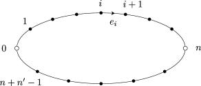
Figure 6.1: The graphical representation of paths of vertices.

There are $n+n^{\prime}$ oriented edges $e_{0},\dots,e_{n+n^{\prime}-1}$ defined by $e_{i}\mathrel{\mathop{:}}=(i,i+1)$ (here, and in the following, $\mathcal{V}_{n,n^{\prime}}$ is taken to be periodic). We denote by $\mathcal{E}_{n,n^{\prime}}\mathrel{\mathop{:}}=\{e_{0},\dots,e_{n+n^{\prime}-1}\}$ the set of edges. In Figure 6.1 the edges are oriented clockwise. Each vertex has an outgoing and an incoming edge, and each edge $e$ has an initial vertex $a(e)$ and final vertex $b(e)$. Moreover, we order the edges using their initial vertices.

Each vertex $i\in\mathcal{V}_{n,n^{\prime}}$ carries a label $x_{i}\in\Lambda_{N}$. The labels $\bm{\mathrm{x}}=(x_{0},\dots,x_{n+n^{\prime}-1})$ are summed over under the restriction $Q_{x}(\bm{\mathrm{x}})=1$, where

$$Q_{x}(\bm{\mathrm{x}})\;\mathrel{\mathop{:}}=\;\delta_{0x_{0}}\delta_{x_{n}x}\prod_{i=0}^{n+n^{\prime}-1}\bm{\mathrm{1}}(1\leqslant\lvert x_{i}-x_{i+1}\rvert\leqslant W)\prod_{i=0}^{n-2}\bm{\mathrm{1}}(x_{i}\neq x_{i+2})\prod_{i=n}^{n+n^{\prime}-2}\bm{\mathrm{1}}(x_{i}\neq x_{i+2})\,.$$

The two last products implement the nonbacktracking condition. We define the unordered pair of labels corresponding to the edge $e$ through

$$\varrho_{\bm{\mathrm{x}}}(e)\;\mathrel{\mathop{:}}=\;\{x_{a(e)},x_{b(e)}\}\,.$$

Next, to each configuration of labels $\bm{\mathrm{x}}=(x_{0},\dots,x_{n+n^{\prime}-1})$ we assign a lumping $\Gamma=\Gamma(\bm{\mathrm{x}})$ of the set of edges $\mathcal{E}_{n,n^{\prime}}$. Here a lumping means a partition of $\mathcal{E}_{n,n^{\prime}}$ or, equivalently, an equivalence relation on $\mathcal{E}_{n,n^{\prime}}$. We use the notation $\Gamma=\{\gamma\}_{\gamma\in\Gamma}$, where $\gamma\in\Gamma$ is lump of $\Gamma$, i.e. an equivalence class. The lumping $\Gamma=\Gamma(\bm{\mathrm{x}})$ associated with the labels $\bm{\mathrm{x}}$ is defined according to the rule that $e$ and $e^{\prime}$ are in the same lump $\gamma\in\Gamma$ if and only if $\varrho_{\bm{\mathrm{x}}}(e)=\varrho_{\bm{\mathrm{x}}}(e^{\prime})$. Let $\widetilde{\mathscr{G}}_{n,n^{\prime}}$ denote the set of lumpings of $\mathcal{E}_{n,n^{\prime}}$ obtained in this manner. Thus we may write

$$\mathbb{E}\,H^{(n)}_{0x}H^{(n^{\prime})}_{x0}\;=\;\sum_{\Gamma\in\widetilde{\mathscr{G}}_{n,n^{\prime}}}V_{x}(\Gamma)\,.$$

Here

$$V_{x}(\Gamma)\;=\;\sideset{}{{}^{*}}{\sum}_{\bm{\mathrm{x}}}Q_{x}(\bm{\mathrm{x}})\,\mathbb{E}\,H_{x_{0}x_{1}}\cdots H_{x_{n+n^{\prime}-1}x_{0}}\,,$$

where the summation is restricted to label configurations yielding the lumping $\Gamma$.

Next, observe that the expectation of a monomial $\prod_{y,z}(H_{yz})^{\nu_{yz}}$ is nonzero if and only if $\nu_{yz}=\nu_{zy}$ for all $y,z$ (here we only use that the law of the matrix entries is invariant under rotations of the complex plane). In particular, $V_{x}(\Gamma)$ vanishes if one lump $\gamma\in\Gamma$ is of odd size. Defining the subset $\mathscr{G}_{n,n^{\prime}}\subset\widetilde{\mathscr{G}}_{n,n^{\prime}}$ of lumpings whose lumps are of even size, we find that

$$\mathbb{E}\,H^{(n)}_{0x}H^{(n^{\prime})}_{x0}\;=\;\sum_{\Gamma\in\mathscr{G}_{n,n^{\prime}}}V_{x}(\Gamma)\,.$$

We summarize the key properties of $\mathscr{G}_{n,n^{\prime}}$.

Lemma 6.1.

Let $\Gamma\in\mathscr{G}_{n,n^{\prime}}$. Then each lump $\gamma\in\Gamma$ is of even size. Moreover, any two edges $e,e^{\prime}\in\gamma$ in the same lump $\gamma$ are separated by either at least two edges or a vertex in $\{0,n\}$ (nonbacktracking property).

Next, we give an explicit expression for $V_{x}(\Gamma)$. We start by assigning to each lump $\gamma\in\Gamma$ an unordered pair of labels $\varrho_{\gamma}$. Then we pick a partition $\pi_{\gamma}$ of $\gamma$ into two subsets of equal size. Abbreviate these families as $\bm{\mathrm{\varrho}}_{\Gamma}=\{\varrho_{\gamma}\}_{\gamma\in\Gamma}$ and $\bm{\mathrm{\pi}}_{\Gamma}=\{\pi_{\gamma}\}_{\gamma\in\Gamma}$. Thus we get

$$V_{x}(\Gamma)\;=\;\sum_{\bm{\mathrm{x}}}Q_{x}(\bm{\mathrm{x}})\sum_{\bm{\mathrm{\varrho}}_{\Gamma}}\sum_{\bm{\mathrm{\pi}}_{\Gamma}}\Biggl{(}{\prod_{\gamma\in\Gamma}\Delta_{\bm{\mathrm{x}}}(\varrho_{\gamma},\pi_{\gamma})}\Biggr{)}\Biggl{(}{\prod_{\gamma\neq\gamma^{\prime}}\bm{\mathrm{1}}(\varrho_{\gamma}\neq\varrho_{\gamma^{\prime}})}\Biggr{)}\,\mathbb{E}H_{x_{0}x_{1}}\cdots H_{x_{n+n^{\prime}-1}x_{0}}\,.$$ (6.1)

Here, for each $\gamma\in\Gamma$, $\varrho_{\gamma}$ ranges over all unordered pairs of labels and $\pi_{\gamma}$ ranges over all partitions of $\gamma$ into two subsets of equal size; $\Delta_{\bm{\mathrm{x}}}(\varrho_{\gamma},\pi_{\gamma})$ is the indicator function of the following event: For all $e\in\gamma$ we have that $\varrho_{\bm{\mathrm{x}}}(e)=\varrho_{\gamma}$, and

$$e,e^{\prime}\in\gamma \pi_{\gamma} \qquad\Longrightarrow\qquad x_{a(e)}\;=\;x_{a(e^{\prime})}\,,\quad x_{b(e)}\;=\;x_{b(e^{\prime})}$$ belong to the same subset of

$$e,e^{\prime}\in\gamma \pi_{\gamma} \qquad\Longrightarrow\qquad x_{a(e)}\;=\;x_{b(e^{\prime})}\,,\quad x_{b(e)}\;=\;x_{a(e^{\prime})}\,.$$ belong to different subsets of

This definition of $\Delta_{\bm{\mathrm{x}}}(\varrho_{\gamma},\pi_{\gamma})$ has the following interpretation. All edges in $\gamma$ (corresponding to matrix elements) have the same unordered pair of labels (and hence represent copies of the same random variable $H_{yz}$ or its complex conjugate). Moreover, each random variable $H_{yz}$ must appear as many times as its complex conjugate; random variables indexed by two edges $e,e^{\prime}\in\gamma$ are identical if $e,e^{\prime}$ belong to the same subset of $\pi_{\gamma}$, and each other’s complex conjugates if $e,e^{\prime}$ belong to different subsets of $\pi_{\gamma}$.

Note that the expectation in (6.1) is equal to

$$\frac{1}{(M-1)^{\bar{n}}}\,,$$ (6.2)

where $\bar{n}\mathrel{\mathop{:}}=\frac{n+n^{\prime}}{2}$. In particular, $V_{x}(\Gamma)\geqslant 0$.

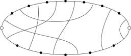
Figure 6.2: A pairing of edges.

An important subset of lumpings of $\mathcal{E}_{n,n^{\prime}}$ is the set of pairings, $\mathscr{P}_{n,n^{\prime}}\subset\mathscr{G}_{n,n^{\prime}}$, which contains all lumpings $\Gamma$ satisfying $\lvert\gamma\rvert=2$ for all $\gamma\in\Gamma$. We call two-element lumps $\sigma\in\mathcal{P}_{n,n^{\prime}}$ bridges. Given a pairing $\Gamma\in\mathscr{P}_{n,n^{\prime}}$, we say that $e$ and $e^{\prime}$ are bridged (in $\Gamma$) if there is a $\sigma\in\Gamma$ such that $\sigma=\{e,e^{\prime}\}$. Bridges are represented graphically by drawing a line, for each $\{e,e^{\prime}\}\in\Gamma$, from the edge $e$ to $e^{\prime}$; see Figure 6.2. Thus a pairing $\Gamma\in\mathscr{P}_{n,n^{\prime}}$ is the edge set of a graph whose vertex set is $\mathcal{E}_{n,n^{\prime}}$. If $\Gamma$ is a pairing, each bridge $\sigma\in\Gamma$ has a unique partition $\pi_{\sigma}$ of its edges, so that the expression (6.1) for $V_{x}(\Gamma)$ may be rewritten in the simpler form

$$V_{x}(\Gamma)\;=\;\sum_{\bm{\mathrm{x}}}Q_{x}(\bm{\mathrm{x}})\Biggl{(}{\prod_{\{e,e^{\prime}\}\in\Gamma}\bm{\mathrm{1}}(x_{a(e)}=x_{b(e^{\prime})})\bm{\mathrm{1}}(x_{b(e)}=x_{a(e^{\prime})})}\Biggr{)}\\ \times\Biggl{(}{\prod_{\sigma\neq\sigma^{\prime}}\prod_{e\in\sigma}\prod_{e^{\prime}\in\sigma^{\prime}}\bm{\mathrm{1}}(\varrho_{\bm{\mathrm{x}}}(e)\neq\varrho_{\bm{\mathrm{x}}}(e^{\prime}))}\Biggr{)}\frac{1}{(M-1)^{\bar{n}}}\,.$$ (6.3)

The main contribution to the expansion is given by the ladder pairing $L_{n}\in\mathscr{P}_{n,n}$. It is defined as

$$L_{n}\;\mathrel{\mathop{:}}=\;\bigl{\{}{\{e_{0},e_{2n-1}\},\{e_{1},e_{2n-2}\},\dots,\{e_{n-1},e_{n}\}}\bigr{\}}\,.$$

The ladder is represented graphically in Figure 6.3.

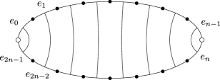
Figure 6.3: The ladder pairing.

7 The non-ladder lumpings

In this section we estimate the contribution of the non-ladder lumpings and show that it vanishes in the limit $W\to\infty$. Let $\mathscr{G}_{n,n^{\prime}}^{*}\subset\mathscr{G}_{n,n^{\prime}}$ denote the set of non-ladder lumpings, i.e. $\mathscr{G}^{*}_{n,n^{\prime}}\mathrel{\mathop{:}}=\mathscr{G}_{n,n^{\prime}}$ if $n\neq n^{\prime}$ and $\mathscr{G}^{*}_{n,n}\mathrel{\mathop{:}}=\mathscr{G}_{n,n}\setminus\{L_{n}\}$. Similarly, let $\mathscr{P}_{n,n^{\prime}}^{*}\mathrel{\mathop{:}}=\mathscr{P}_{n,n^{\prime}}\cap\mathscr{G}^{*}_{n,n^{\prime}}$ denote the set of non-ladder pairings.

We shall prove the following result.

Proposition 7.1.

Let $0<\kappa<1/3$ and pick a $\beta$ satisfying $0<\beta<2/3-2\kappa$. Then there is a constant $C$ such that

$$\sum_{x}\sum_{n,n\geqslant 0}\lvert a_{n}(\eta T)\,a_{n^{\prime}}(\eta T)\rvert\sum_{\Gamma\in\mathscr{G}^{*}_{n,n^{\prime}}}V_{x}(\Gamma)\;\leqslant\;\frac{C}{W^{d\beta}}\,,$$

for $W$ larger than some $W_{0}(T,\kappa)$ and $N\geqslant W^{1+d/6}$.

The rest of this section is devoted to the proof of Proposition 7.1.

7.1 Controlling the non-pairings

Replacing the expectation in (6.1) with (6.2) we get

$$V_{x}(\Gamma)\;=\;\sum_{\bm{\mathrm{x}}}Q_{x}(\bm{\mathrm{x}})\sum_{\bm{\mathrm{\varrho}}_{\Gamma}}\sum_{\bm{\mathrm{\pi}}_{\Gamma}}\Biggl{(}{\prod_{\gamma\in\Gamma}\Delta_{\bm{\mathrm{x}}}(\varrho_{\gamma},\pi_{\gamma})}\Biggr{)}\Biggl{(}{\prod_{\gamma\neq\gamma^{\prime}}\bm{\mathrm{1}}(\varrho_{\gamma}\neq\varrho_{\gamma^{\prime}})}\Biggr{)}\,\frac{1}{(M-1)^{\bar{n}}}\,.$$

We start by estimating the sum over all lumpings $\Gamma\in\mathscr{G}_{n,n^{\prime}}^{*}$ in terms of a sum over all pairings $\Gamma\in\mathscr{P}_{n,n^{\prime}}^{*}$. Let us define

$$R_{x}(\Gamma)\;\mathrel{\mathop{:}}=\;\sum_{\bm{\mathrm{x}}}Q_{x}(\bm{\mathrm{x}})\sum_{\bm{\mathrm{\varrho}}_{\Gamma}}\sum_{\bm{\mathrm{\pi}}_{\Gamma}}\Biggl{(}{\prod_{\gamma\in\Gamma}\Delta_{\bm{\mathrm{x}}}(\varrho_{\gamma},\pi_{\gamma})}\Biggr{)}\,\frac{1}{(M-1)^{\bar{n}}}\,.$$ (7.1)

Lemma 7.2.

For all $n,n^{\prime}\in\mathbb{N}$ we have

$$\sum_{\Gamma\in\mathscr{G}_{n,n^{\prime}}^{*}}V_{x}(\Gamma)\;\leqslant\;\sum_{\Gamma\in\mathscr{P}_{n,n^{\prime}}^{*}}R_{x}(\Gamma)\,.$$

Proof.

Let $\varrho_{\gamma}$ and $\pi_{\gamma}$ be given for each $\gamma\in\Gamma$. For each $\gamma$, pick any pairing $\Sigma_{\gamma}$ of $\gamma$ that is compatible with $\pi_{\gamma}$ in the sense that, for each bridge $\sigma\in\Sigma_{\gamma}$, the two edges of $\sigma$ belong to different subsets of $\pi_{\gamma}$. If $n=n^{\prime}$, we additionally require that not all $\Sigma_{\gamma}$’s are subsets of the Ladder $L_{n}$ (such a choice is always possible). Next, set $\varrho_{\sigma}=\varrho_{\gamma}$ for all $\sigma\in\Sigma_{\gamma}$. Note that each bridge $\sigma$ carries a unique partition $\pi_{\sigma}$. It is then easy to see that for any pairing $\Sigma_{\gamma}$ as above, we have

$$\Delta_{\bm{\mathrm{x}}}(\varrho_{\gamma},\pi_{\gamma})\;\leqslant\;\prod_{\sigma\in\Sigma_{\gamma}}\Delta_{\bm{\mathrm{x}}}(\varrho_{\sigma},\pi_{\sigma})\,.$$

Thus, by partitioning each $\gamma\in\Gamma$ into bridges, we see that each term in $\sum_{\Gamma\in\mathscr{G}_{n,n^{\prime}}^{*}}V_{x}(\Gamma)$ is bounded by a corresponding term in $\sum_{\Gamma\in\mathscr{P}_{n,n^{\prime}}^{*}}R_{x}(\Gamma)$. In fact, there is an overcounting arising from the different ways of partitioning $\gamma$ into bridges. ∎

Because of Lemma 7.2 we may restrict ourselves to pairings. We estimate $\sum_{\Gamma\in\mathscr{P}_{n,n^{\prime}}^{*}}R_{x}(\Gamma)$. If $\Gamma$ is a pairing we may write, just like (6.3), the expression (7.1) in the simpler form

$$R_{x}(\Gamma)\;=\;\sum_{\bm{\mathrm{x}}}Q_{x}(\bm{\mathrm{x}})\Biggl{(}{\prod_{\{e,e^{\prime}\}\in\Gamma}\bm{\mathrm{1}}(x_{a(e)}=x_{b(e^{\prime})})\bm{\mathrm{1}}(x_{b(e)}=x_{a(e^{\prime})})}\Biggr{)}\,\frac{1}{(M-1)^{\bar{n}}}\,.$$ (7.2)

7.2 Collapsing of parallel bridges

Let us introduce the set $\overline{\mathscr{P}}\!\,^{*}_{n,n^{\prime}}$, defined as the set of all non-ladder pairings of $\mathcal{E}_{n,n^{\prime}}$. Clearly, $\mathscr{P}^{*}_{n,n^{\prime}}$ is a proper subset of $\overline{\mathscr{P}}\!\,^{*}_{n,n^{\prime}}$ (due to the nonbacktracking condition of Lemma 6.1 which is imposed on pairings in $\mathscr{P}^{*}_{n,n^{\prime}}$).

Let $n,n^{\prime}\geqslant 0$ and $\Gamma\in\overline{\mathscr{P}}\!\,^{*}_{n,n^{\prime}}$. For any $i,j$, we say that the two bridges $\{e_{i},e_{j}\}$ and $\{e_{i+1},e_{j-1}\}$ of $\Gamma$ are parallel if $i+1,j\notin\{0,n\}$; see Figure 7.1. Two parallel bridges may be collapsed to obtain a new pairing $\Gamma^{\prime}$ of a smaller set of edges, in which the parallel bridges are replaced by a single bridge. More precisely: We obtain $\Gamma^{\prime}\in\overline{\mathscr{P}}\!\,^{*}_{m,m^{\prime}}$ from $\Gamma\in\overline{\mathscr{P}}\!\,^{*}_{n,n^{\prime}}$ by removing the vertices $i+1$ and $j$, by creating the edges $(i,i+2)$ and $(j-1,j+1)$, and by bridging them. Finally, we rename the vertices using the increasing integers $0,1,2,\dots,n+n^{\prime}-3$; by definition, the new name of the vertex $n$ is $m$, and $m^{\prime}$ is defined through $m+m^{\prime}+2=n+n^{\prime}$.

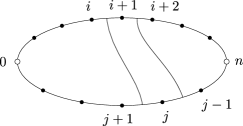
Figure 7.1: Two parallel bridges.

The converse operation of collapsing bridges, expanding bridges, is self-explanatory.

In the next lemma we iterate the above procedure $\Gamma\mapsto\Gamma^{\prime}$ until all parallel bridges have been collapsed.

Lemma 7.3.

Let $\Gamma\in\mathscr{P}^{*}_{n,n^{\prime}}$. Then there exist $m\leqslant n$, $m^{\prime}\leqslant n^{\prime}$, and a pairing $S(\Gamma)\in\overline{\mathscr{G}}\!\,^{*}_{m,m^{\prime}}$ containing no parallel bridges, such that $\Gamma$ may be obtained from $S(\Gamma)$ by successively expanding bridges. This defines $S(\Gamma)$ uniquely.

Proof.

Successively collapse all parallel bridges in $\Gamma$; see Figure 7.2. The result is clearly independent of the order in which this is done.

Figure 7.2: Collapsing parallel bridges to obtain the skeleton pairing.

∎

We call the pairing $\Sigma=S(\Gamma)$ the skeleton of $\Gamma$. The set of skeleton pairings of the edges $\mathcal{E}_{m,m^{\prime}}$ is denoted by

$$\mathscr{S}^{*}_{m,m^{\prime}}\;\mathrel{\mathop{:}}=\;\bigcup_{n,n^{\prime}\geqslant 0}\bigl{\{}{S(\Gamma)\,:\,\Gamma\in\mathscr{P}^{*}_{n,n^{\prime}}}\bigr{\}}\cap\overline{\mathscr{P}}\!\,^{*}_{m,m^{\prime}}\,.$$

Note that $\mathscr{S}^{*}_{m,m^{\prime}}$ is in general not a subset of $\mathscr{P}^{*}_{m,m^{\prime}}$. The following lemma summarizes the key properties of $\mathscr{S}^{*}_{m,m^{\prime}}$.

Lemma 7.4.

1. Each $\Sigma\in\mathscr{S}^{*}_{m,m^{\prime}}$ contains no parallel bridges.

2. Let $\Sigma\in\mathscr{S}^{*}_{m,m^{\prime}}$ and $\sigma=\{e,e^{\prime}\}\in\Sigma$. Then $e,e^{\prime}$ are adjacent only if $e\cap e^{\prime}\in\{0,m\}$.

3. If $\bar{m}\mathrel{\mathop{:}}=\frac{m+m^{\prime}}{2}=1$ then $\mathscr{S}^{*}_{m,m^{\prime}}=\emptyset$.

Proof.

Statement (i) follows immediately from the definition of $S(\Gamma)$. Statement (ii) is a consequence of the nonbacktracking property of pairings in $\mathscr{P}^{*}_{n,n^{\prime}}$, i.e. Lemma 6.1. To see this, let $\Sigma\in\mathscr{S}^{*}_{m,m^{\prime}}$ be of the form $\Sigma=S(\Gamma)$ for some $\Gamma\in\mathscr{P}^{*}_{n,n^{\prime}}$. If $\Sigma=S(\Gamma)$ contains a bridge $\{e,e^{\prime}\}$ consisting of two consecutive edges $e,e^{\prime}$, then $\Gamma$ must also contain a bridge $\{f,f^{\prime}\}$ consisting of two consecutive edges $f,f^{\prime}$. If $e\cap e^{\prime}\notin\{0,m\}$, then $f\cap f^{\prime}\notin\{0,n\}$, in contradiction to Lemma 6.1. Statement (iii) is an immediate consequence of (ii) and the requirement that $L_{1}\notin\mathscr{S}^{*}_{1,1}$. ∎

7.3 Contribution of parallel bridges

For given $n$ and $n^{\prime}$, we estimate $\sum_{\Gamma\in\mathscr{P}^{*}_{n,n^{\prime}}}R_{x}(\Gamma)$ by summing over skeleton pairings $\Sigma$, followed by summing over all possible ways of expanding the bridges of $\Sigma$.

We observe that a pairing $\Gamma\in\mathscr{P}^{*}_{n,n^{\prime}}$ is uniquely determined by its skeleton $\Sigma=S(\Gamma)\in\mathscr{S}^{*}_{m,m^{\prime}}$ for some positive integers $m,m^{\prime}$ as well as a family $\bm{\mathrm{\ell}}_{\Sigma}=\{\ell_{\sigma}\}_{\sigma\in\Sigma}$ satisfying $\lvert\bm{\mathrm{\ell}}_{\Sigma}\rvert=\bar{n}$, where $\ell_{\sigma}$ encodes the number of parallel bridges that were collapsed to form the bridge $\sigma$. Here $\ell_{\sigma}\geqslant 1$ is a positive integer and $\lvert\bm{\mathrm{\ell}}_{\Sigma}\rvert\mathrel{\mathop{:}}=\sum_{\sigma\in\Sigma}\ell_{\sigma}$. Let $G_{\bm{\mathrm{\ell}}_{\Sigma}}(\Sigma)$ denote the pairing obtained from $\Sigma$ by expanding the bridge $\sigma$ into $\ell_{\sigma}$ parallel bridges, for each $\sigma\in\Sigma$. Thus $\Gamma$ may be recovered from its skeleton through $\Gamma=G_{\bm{\mathrm{\ell}}_{\Sigma}}(\Sigma)$ for a unique family $\bm{\mathrm{\ell}}_{\Sigma}$. For given $p\in\mathbb{N}$, the sum over all pairings $\Gamma$ satisfying $\lvert\Gamma\rvert=p$ therefore becomes

$$\sum_{n+n^{\prime}=2p}\;\sum_{\Gamma\in\mathscr{P}_{n,n^{\prime}}^{*}}R_{x}(\Gamma)\;=\;\sum_{m+m^{\prime}\leqslant 2p}\;\sum_{\Sigma\in\mathscr{S}^{*}_{m,m^{\prime}}}\;\sum_{\bm{\mathrm{\ell}}_{\Sigma}\,:\,\lvert\bm{\mathrm{\ell}}_{\Sigma}\rvert=p}R_{x}(G_{\bm{\mathrm{\ell}}_{\Sigma}}(\Sigma))\,.$$ (7.3)

Next, we define and estimate the contribution to $R_{x}(\Gamma)$ of a set of $\ell$ parallel bridges. Let $\ell\geqslant 1$, and two labels $y,z$ be given. Then we define

$$D_{\ell}(y,z)\;\mathrel{\mathop{:}}=\;\sum_{x_{0},\dots,x_{\ell}}\delta_{x_{0}y}\delta_{x_{\ell}z}\prod_{i=0}^{\ell-1}\bm{\mathrm{1}}(1\leqslant\lvert x_{i}-x_{i+1}\rvert\leqslant W)\,.$$

Thus, $D_{\ell}(y,z)$ is equal to the number of paths of length $\ell$ from $y$ to $z$, whereby each step takes values in $\{x\,:\,1\leqslant\lvert x\rvert\leqslant W\}$. (We could also have included the nonbacktracking restriction in the definition of $D_{\ell}$, but this is not needed as we only want an upper bound on $R_{x}(\Sigma)$). Graphically, $D_{\ell}$ corresponds to the contribution of $\ell$ parallel bridges; see Figure 7.3.

Figure 7.3: Summing up $\ell$ parallel bridges.

We need the following straightforward properties of $D_{\ell}$.

Lemma 7.5.

Let $\ell\in\mathbb{N}$. Then for each $y$ we have

$$\sum_{z}D_{\ell}(y,z)\;=\;M^{\ell}\,.$$

Moreover, for each $y$ and $z$ we have

$$D_{\ell}(y,z)\;\leqslant\;M^{\ell-1}\,.$$

as well as

$$D_{\ell}(y,z)\;\leqslant\;\frac{C}{\ell^{d/2}}M^{\ell-1}+\frac{C}{N^{d}}M^{\ell}\,.$$

for some constant $C$.

Proof.

The first two statements are obvious. The last follows from a standard local central limit theorem; see for instance the proof in [42]. ∎

7.4 Orbits of vertices

Fix $\Gamma\in\mathscr{P}^{*}_{n,n^{\prime}}$. We observe that the product in (7.2) may be interpreted as an indicator function that fixes labels along paths of vertices. To this end, we define a map $\tau\equiv\tau_{\,\Gamma}$ on the vertex set $\mathcal{V}_{n,n^{\prime}}$. Start with a vertex $i\in\mathcal{V}_{n,n^{\prime}}$. Let $e$ be the outgoing edge of $i$ (i.e. $e=(i,i+1)$), and $e^{\prime}$ the edge bridged by $\Gamma$ to $e$. Then we define $\tau i$ as the final vertex of $e^{\prime}$ (i.e. $e^{\prime}=(\tau i-1,\tau i)$). Thus the product in (7.2) may be rewritten as

$$\prod_{\{e,e^{\prime}\}\in\Gamma}\bm{\mathrm{1}}(x_{a(e)}=x_{b(e^{\prime})})\bm{\mathrm{1}}(x_{b(e)}=x_{a(e^{\prime})})\;=\;\prod_{i\in\mathcal{V}_{n,n^{\prime}}}\delta_{x_{i}x_{\tau i}}\,.$$

Starting from any vertex $i\in\mathcal{V}_{n,n^{\prime}}$ we construct a path $(i,\tau i,\tau^{2}i,\dots)$. In this fashion the set of vertices is partitioned into orbits of $\tau$; see Figure 7.4. Let $[i]\subset\mathcal{V}_{n,n^{\prime}}$ denote the orbit of the vertex $i\in\mathcal{V}_{n,n^{\prime}}$.

Figure 7.4: Construction of the orbit $[i]$ of the vertex $i$.

Next, let $\Sigma=S(\Gamma)\in\mathscr{S}^{*}_{m,m^{\prime}}$ be the skeleton pairing of $\Gamma$, and let the family $\bm{\mathrm{\ell}}_{\Sigma}$ be defined through $\Gamma=G_{\bm{\mathrm{\ell}}_{\Sigma}}(\Sigma)$. The map $\tau\equiv\tau_{\,\Sigma}$ on the skeleton pairing $\Sigma$ is defined exactly as for $\Gamma$ above. In order to sum over all labels $\bm{\mathrm{x}}=(x_{0},\dots,x_{n+n^{\prime}-1})$ in the expression for $R_{x}(G_{\bm{\mathrm{\ell}}_{\Sigma}}(\Sigma))$, we split the set of labels $\bm{\mathrm{x}}$ into two parts: labels of vertices between two parallel bridges, and labels associated with vertices of $\Sigma$. In order to make this precise, we need the following definitions.

Let $Z(\Sigma)$ be the set of orbits of $\Sigma$. It contains the distinguished orbits $[0]$ and $[m]$, which receive the labels $0$ and $x$ respectively. (Note that we may have $[0]=[m]$, in which case $x$ must be $0$.) We assign a label $y_{\zeta}$ to each orbit $\zeta\in Z(\Sigma)$, and define the family $\bm{\mathrm{y}}_{\Sigma}\mathrel{\mathop{:}}=\{y_{\zeta}\}_{\zeta\in Z(\Sigma)}$. Each bridge $\sigma\in\Sigma$ “sits between two orbits” $\zeta_{1}(\sigma)$ and $\zeta_{2}(\sigma)$ . More precisely, let $e=(i,i+1)\in\sigma$ be the smaller edge of $\sigma$. Then we set $\zeta_{1}(\sigma)\mathrel{\mathop{:}}=[i]$ and $\zeta_{2}(\sigma)\mathrel{\mathop{:}}=[i+1]$. (Note that using the larger edge of $\sigma$ in this definition would simply exchange $\zeta_{1}(\sigma)$ and $\sigma_{2}(\sigma)$; this is of no consequence for the following.)

Lemma 7.6.

For given $\Sigma\in\mathscr{S}^{*}_{m,m^{\prime}}$, $\bm{\mathrm{\ell}}_{\Sigma}$, and $\Gamma=G_{\bm{\mathrm{\ell}}_{\Sigma}}(\Sigma)\in\mathscr{P}^{*}_{n,n^{\prime}}$ we have

$$R_{x}(\Gamma)\;\leqslant\;\frac{1}{(M-1)^{\bar{n}}}\sum_{\bm{\mathrm{y}}_{\Sigma}}\bm{\mathrm{1}}(0=y_{[0]})\bm{\mathrm{1}}(x=y_{[m]})\prod_{\sigma\in\Sigma}D_{\ell_{\sigma}}(y_{\zeta_{1}(\sigma)},y_{\zeta_{2}(\sigma)})\,.$$ (7.4)

Proof.

The left-hand side of (7.4) is given by the expression (7.2). The summation over all $x_{i}$’s between parallel bridges of $\Gamma$ is contained in the factors $D_{\ell}$, and the summation over all the remaining $x_{i}$’s is replaced by the sum over $\bm{\mathrm{y}}_{\Sigma}$. We relaxed the nonbacktracking condition in $Q_{x}(\bm{\mathrm{x}})$ to obtain an upper bound. ∎

Next, let $Z^{*}(\Sigma)\mathrel{\mathop{:}}=Z(\Sigma)\setminus\{[0]\}$ and define $L(\Sigma)\mathrel{\mathop{:}}=\lvert Z^{*}(\Sigma)\rvert$. The set $Z^{*}(\Sigma)$ is the set of orbits whose label is summed over in $\sum_{x}R_{x}(\Gamma)$. The following lemma gives an upper bound on $L(\Sigma)$. It states, roughly, that the number of orbits (or free labels) is bounded by $2\bar{m}/3$; we refer to it as the $2/3$ rule. Compare this bound with the trivial bound $L(\Sigma)\leqslant\bar{m}$, which would be sharp if $\Sigma$ were allowed to have parallel bridges.

Lemma 7.7 (The $2/3$ rule).

Let $\Sigma\in\mathscr{S}_{m,m^{\prime}}^{*}$. Then $L(\Sigma)\leqslant\frac{2\bar{m}}{3}+\frac{1}{3}$.

Proof.

Let $Z^{\prime}(\Sigma)\mathrel{\mathop{:}}=Z(\Sigma)\setminus\{[0],[m]\}$. We show that every orbit $\zeta\in Z^{\prime}(\Sigma)$ consists of at least 3 vertices. Let $i\in\mathcal{V}_{m,m^{\prime}}$ belong to $\zeta\in Z^{\prime}(\Sigma)$. Then, by Lemma 7.4 (ii), we have that $\tau i\neq i$. By assumption, $\tau i\notin\{0,m\}$. Hence $\tau^{2}i\neq i$, for otherwise $\Sigma$ would have two parallel bridges, in contradiction to Lemma 7.4 (i). Therefore the orbit of $\tau$ contains at least 3 vertices. Note that there are orbits containing exactly 3 vertices, as depicted in Figure 7.4.

The total number of vertices of $\Sigma$ not including the vertices $0$ and $m$ is $2\bar{m}-2$, so that we get

$$3\lvert Z^{\prime}(\Sigma)\rvert\;\leqslant\;2\bar{m}-2\,.$$

The claim follows from the bound $\lvert Z^{*}(\Sigma)\rvert\leqslant\lvert Z^{\prime}(\Sigma)\rvert+1$. ∎

7.5 Bound on $R_{x}(\Gamma)$

As in the previous subsection, we fix $\Gamma\in\mathscr{P}^{*}_{n,n^{\prime}}$, $\Sigma=S(\Gamma)\in\mathscr{S}^{*}_{m,m^{\prime}}$, and $\bm{\mathrm{\ell}}_{\Sigma}$ satisfying $\Gamma=G_{\bm{\mathrm{\ell}}_{\Sigma}}(\Sigma)$.

We start by observing that the product in (7.4) may be rewritten in terms of a multigraph $\Pi(\Sigma)$ on the vertex set $Z(\Sigma)$. Each factor $D_{\ell_{\sigma}}(y_{\zeta_{1}(\sigma)},y_{\zeta_{2}(\sigma)})$ yields an edge connecting the orbits $\zeta_{1}$ and $\zeta_{2}$. In other words, there is a one-to-one map, which we denote by $\phi$, between bridges of $\Sigma$ and edges of $\Pi(\Sigma)$; each bridge $\sigma\in\Sigma$ gives rise to an edge $\phi(\sigma)$ of $\Pi(\Sigma)$ connecting $\zeta_{1}(\sigma)$ and $\zeta_{2}(\sigma)$. See Figure 7.5 for an example of such a multigraph.

Figure 7.5: Left: a skeleton pairing $\Sigma$ giving rise to $5$ orbits indexed by $Z(\Sigma)=\{1,\dots,5\}$; the bridges in $\Sigma_{T}$, for one possible choice of $\Sigma_{T}$, are drawn using thick lines. Right: the corresponding multigraph on the vertex set $Z(\Sigma)$; the edges in $\phi(\Sigma_{T})$ are drawn using thick lines.

Lemma 7.8.

There is a subset of bridges $\Sigma_{T}\subset\Sigma$ of size $\lvert\Sigma_{T}\rvert=L(\Sigma)$, such that, in the subgraph of $\Pi(\Sigma)$ with the edge set $\phi(\Sigma_{T})$, each orbit $\zeta\in Z^{*}(\Sigma)$ is connected to $[0]$.

Proof.

Starting from $\zeta_{0}=[0]$, we construct a sequence of orbits $\zeta_{0},\zeta_{1},\dots,\zeta_{L(\Sigma)}$, and a sequence of bridges $\sigma_{1},\dots,\sigma_{L(\Sigma)}$, with the property that for all $k=1,\dots,L(\Sigma)$ there is a $k^{\prime}<k$ such that $\zeta_{k}$ and $\zeta_{k^{\prime}}$ are connected by $\phi(\sigma_{k})$.

Assume that $\zeta_{0},\dots,\zeta_{k-1}$ have already been constructed. Let $i$ be the smallest vertex of $\mathcal{V}_{m,m^{\prime}}\setminus(\zeta_{0}\cup\cdots\cup\zeta_{k-1})$. Then we set $\zeta_{k}=[i]$. By construction, the vertex $i-1$ belongs to an orbit $\zeta_{k^{\prime}}$ for some $k^{\prime}<k$. Set $\sigma_{k}$ to be the bridge containing $\{i-1,i\}$. Hence, by definition of $\Pi(\Sigma)$, we see that $\zeta_{k}$ and $\zeta_{k^{\prime}}$ are connected by $\phi(\sigma_{k})$.

The set $\Sigma_{T}$ is given by $\{\sigma_{1},\dots,\sigma_{L(\Sigma)}\}$. ∎

Because $\lvert\Sigma_{T}\rvert=L(\Sigma)$, the subgraph of $\Pi(\Sigma)$ with the edge set $\phi(\Sigma_{T})$ is a tree that connects all orbits in $Z^{*}(\Sigma)$ to $[0]$. Let us call this tree $\mathcal{T}(\Sigma)$. Its root is $[0]$.

Next, we observe that

$$\lvert\Sigma\setminus\Sigma_{T}\rvert\;\geqslant\;1\,.$$ (7.5)

Indeed, using Lemma 7.7 and $\bar{m}\geqslant 2$ we find

$$\lvert\Sigma\setminus\Sigma_{T}\rvert\;=\;\bar{m}-L(\Sigma)\;\geqslant\;\frac{\bar{m}}{3}-\frac{1}{3}\;\geqslant\;\frac{1}{3}\,.$$ (7.6)

We now estimate (7.4) as follows. Each factor indexed by $\sigma\in\Sigma\setminus\Sigma_{T}$ is estimated by $\sup_{y,z}D_{\ell_{\sigma}}(y,z)$. As it turns out, we need to exploit the heat kernel decay for at least one bridge in $\Sigma\setminus\Sigma_{T}$. Pick a bridge $\bar{\sigma}\in\Sigma\setminus\Sigma_{T}$ (By (7.5) there is such a bridge). Using Lemma 7.5, we estimate

$$\sup_{y,z}D_{\ell_{\sigma}}(y,z) \;\leqslant\;M^{\ell_{\sigma}-1} \text{if }\sigma\in\Sigma\setminus(\Sigma_{T}\cup\{\bar{\sigma}\})\,,$$ (7.7a)

$$\sup_{y,z}D_{\ell_{\sigma}}(y,z) \;\leqslant\;\frac{C}{\ell_{\sigma}^{d/2}}M^{\ell_{\sigma}-1}+\frac{C}{N^{d}}M^{\ell_{\sigma}} \text{if }\sigma=\bar{\sigma}\,.$$ (7.7b)

Since $N\geqslant WM^{1/6}$ and $M\sim CW^{d}$ we find

$$\frac{C}{\ell_{\bar{\sigma}}^{d/2}}M^{\ell_{\bar{\sigma}}-1}+\frac{C}{N^{d}}M^{\ell_{\bar{\sigma}}}\;\leqslant\;CM^{\ell_{\bar{\sigma}}-1}\biggl{(}{\frac{1}{\ell_{\bar{\sigma}}^{1/2}}+\frac{1}{M^{1/6}}}\biggr{)}\,$$

where we replaced $d$ with $1$ to obtain an upper bound. Thus we get

$$\sum_{x}R_{x}(\Gamma)\;\leqslant\;\frac{C}{(M-1)^{\bar{n}}}\biggl{(}{\frac{1}{\ell_{\bar{\sigma}}^{1/2}}+\frac{1}{M^{1/6}}}\biggr{)}\prod_{\sigma\in\Sigma\setminus\Sigma_{T}}M^{\ell_{\sigma}-1}\sum_{\bm{\mathrm{y}}_{\Sigma}}\bm{\mathrm{1}}(0=y_{[0]})\prod_{\sigma\in\Sigma_{T}}D_{\ell_{\sigma}}(y_{\zeta_{1}(\sigma)},y_{\zeta_{2}(\sigma)})\,.$$

We perform the summation over $\bm{\mathrm{y}}_{\Sigma}$ by starting at the leaves of $\mathcal{T}(\Sigma)$ and moving towards the root $[0]$. Each vertex $\zeta$ of $\mathcal{T}(\Sigma)$ carries a label $y_{\zeta}$. Let us choose a leaf $\zeta$ of $\mathcal{T}(\Sigma)$, and denote by $\zeta^{\prime}$ the parent of $\zeta$ in $\mathcal{T}(\Sigma)$. Let $\sigma\in\Sigma$ be the (unique) bridge such that $\phi(\sigma)$ connects $\zeta$ and $\zeta^{\prime}$. Then summation over $y_{\zeta}$ yields the factor

$$\sum_{y_{\zeta}}D_{\ell_{\sigma}}(y_{\zeta},y_{\zeta^{\prime}})\;=\;M^{\ell_{\sigma}}\,,$$ (7.8)

by Lemma 7.5. Continuing in this manner until we reach the root, we find

$$\sum_{x}R_{x}(\Gamma) \;\leqslant\;\frac{C}{(M-1)^{\bar{n}}}\biggl{(}{\frac{1}{\ell_{\bar{\sigma}}^{1/2}}+\frac{1}{M^{1/6}}}\biggr{)}\prod_{\sigma\in\Sigma\setminus\Sigma_{T}}M^{\ell_{\sigma}-1}\prod_{\sigma\in\Sigma_{T}}M^{\ell_{\sigma}}$$

$$\;=\;C\,\biggl{(}{\frac{M}{M-1}}\biggr{)}^{\bar{n}}\biggl{(}{\frac{1}{\ell_{\bar{\sigma}}^{1/2}}+\frac{1}{M^{1/6}}}\biggr{)}\frac{1}{M^{\lvert\Sigma\setminus\Sigma_{T}\rvert}}\,.$$

Now (7.6) implies

$$\lvert\Sigma\setminus\Sigma_{T}\rvert\;\geqslant\;\frac{\bar{m}}{3}-\frac{1}{3}\,,$$

so that

$$\sum_{x}R_{x}(\Gamma)\;\leqslant\;C\biggl{(}{\frac{M}{M-1}}\biggr{)}^{\bar{n}}\biggl{(}{\frac{1}{\ell_{\bar{\sigma}}^{1/2}}+\frac{1}{M^{1/6}}}\biggr{)}\frac{M^{1/3}}{M^{\bar{m}/3}}\,.$$ (7.9)

Notice that (7.9) results from an $\ell^{1}$-$\ell^{\infty}$-summation procedure, where the $\ell^{1}$-bound (7.8) was used for propagators associated with bridges in $\Sigma_{T}$, and the $\ell^{\infty}$-bound (7.7) for propagators associated with bridges in $\Sigma\setminus\Sigma_{T}$. The bound (7.7a) is a simple power counting bound; the bound (7.7b), improved by the heat kernel decay, is used only for one bridge. Note that in the original setup (2.1) each row and column of $H$ contains $M$ nonzero entries $H_{xy}$, whose positions are determined by the condition $1\leqslant\lvert x-y\rvert\leqslant W$. If we removed this last condition and only required that each row and column contain $M$ nonzero entries in arbitrary locations off the diagonal, then all bounds relying solely on power counting would remain valid. In particular, (7.9) would be valid without the factor $\ell_{\bar{\sigma}}^{-1/2}+M^{-1/6}$, which results from the heat kernel decay associated with the special band structure.

7.6 Sum over pairings

We may now estimate $\sum_{n+n^{\prime}=2p}\sum_{\Gamma\in\mathscr{P}_{n,n^{\prime}}^{*}}\sum_{x}R_{x}(\Gamma)$ for fixed $p$. Let first $p,m,m^{\prime}\geqslant 0$ and $\Sigma\in\mathscr{S}^{*}_{m,m^{\prime}}$. Then (7.9) yields

$$\sum_{\bm{\mathrm{\ell}}_{\Sigma}\,:\,\lvert\bm{\mathrm{\ell}}_{\Sigma}\rvert=p}\sum_{x}R_{x}(G_{\bm{\mathrm{\ell}}_{\Sigma}}(\Sigma))\;\leqslant\;C\biggl{(}{\frac{M}{M-1}}\biggr{)}^{p}\frac{M^{1/3}}{M^{\bar{m}/3}}\sum_{\bm{\mathrm{\ell}}_{\Sigma}\,:\,\lvert\bm{\mathrm{\ell}}_{\Sigma}\rvert=p}\biggl{(}{\frac{1}{\ell_{\bar{\sigma}}^{1/2}}+\frac{1}{M^{1/6}}}\biggr{)}\,.$$

The sum on the right-hand side is equal to

$$\sum_{\ell_{1}+\cdots+\ell_{\bar{m}}=p}\biggl{(}{\frac{1}{\ell_{1}^{1/2}}+\frac{1}{M^{1/6}}}\biggr{)} \;=\;\sum_{\ell_{1}=1}^{p-\bar{m}+1}\biggl{(}{\frac{1}{\ell_{1}^{1/2}}+\frac{1}{M^{1/6}}}\biggr{)}\sum_{\ell_{2}+\cdots+\ell_{\bar{m}}=p-\ell_{1}}1$$

$$\;\leqslant\;\sum_{\ell_{1}=1}^{p}\biggl{(}{\frac{1}{\ell_{1}^{1/2}}+\frac{1}{M^{1/6}}}\biggr{)}\binom{p-\ell_{1}-1}{\bar{m}-2}$$

$$\;\leqslant\;C\biggl{(}{\frac{1}{p^{1/2}}+\frac{1}{M^{1/6}}}\biggr{)}\frac{p^{\bar{m}-1}}{(\bar{m}-2)!}\,.$$

Next, we note that

$$\lvert\mathscr{S}^{*}_{m,m^{\prime}}\rvert\;\leqslant\;(2\bar{m}-1)(2\bar{m}-3)\cdots 3\cdot 1\;\leqslant\;2^{\bar{m}}\,\bar{m}\,!\,.$$

This expresses the fact that the first edge of $\Sigma$ can be bridged with at most $(2\bar{m}-1)$ edges, the next remaining edge with at most $(2\bar{m}-3)$ edges, and so on. Therefore (7.3) and Lemma 7.4 (iii) yield

$$\sum_{n+n^{\prime}=2p}\;\sum_{\Gamma\in\mathscr{P}_{n,n^{\prime}}^{*}}\sum_{x}R_{x}(\Gamma) \;\leqslant\;C\sum_{4\leqslant m+m^{\prime}\leqslant 2p}2^{\bar{m}}\bar{m}!\biggl{(}{\frac{M}{M-1}}\biggr{)}^{p}\frac{M^{1/3}}{M^{\bar{m}/3}}\frac{p^{\bar{m}-1}}{(\bar{m}-2)!}\biggl{(}{\frac{1}{p^{1/2}}+\frac{1}{M^{1/6}}}\biggr{)}$$

$$\;\leqslant\;C\frac{M^{1/3}}{p}\biggl{(}{\frac{1}{p^{1/2}}+\frac{1}{M^{1/6}}}\biggr{)}\biggl{(}{\frac{M}{M-1}}\biggr{)}^{p}\sum_{4\leqslant m+m^{\prime}\leqslant 2p}\bar{m}^{2}2^{\bar{m}}\biggl{(}{\frac{p}{M^{1/3}}}\biggr{)}^{\bar{m}}$$

$$\;\leqslant\;\frac{M^{1/3}}{p}\biggl{(}{\frac{1}{p^{1/2}}+\frac{1}{M^{1/6}}}\biggr{)}\biggl{(}{\frac{M}{M-1}}\biggr{)}^{p}\sum_{\bar{m}=2}^{p}\biggl{(}{\frac{Cp}{M^{1/3}}}\biggr{)}^{\bar{m}}\,.$$

Thus, Lemma 7.2 yields

$$\sum_{n+n^{\prime}=2p}h_{n,n^{\prime}}\;\leqslant\;\frac{M^{1/3}}{p}\biggl{(}{\frac{1}{p^{1/2}}+\frac{1}{M^{1/6}}}\biggr{)}\biggl{(}{\frac{M}{M-1}}\biggr{)}^{p}\sum_{r=2}^{p}\biggl{(}{\frac{Cp}{M^{1/3}}}\biggr{)}^{r}\,,$$ (7.10)

where we abbreviated

$$h_{n,n^{\prime}}\;\mathrel{\mathop{:}}=\;\sum_{\Gamma\in\mathscr{G}^{*}_{n,n^{\prime}}}\sum_{x}V_{x}(\Gamma)\,.$$

7.7 Conclusion of the proof

In this subsection we complete the proof of Proposition 7.1 by showing that the error

$$E_{W}\;\mathrel{\mathop{:}}=\;\sum_{n,n^{\prime}}\big{\lvert}a_{n}(\eta T)\,a_{n^{\prime}}(\eta T)\big{\rvert}\,h_{n,n^{\prime}}$$ (7.11)

satisfies $E_{W}=o(1)$ as $W\to\infty$, uniformly in $N\geqslant W^{1+d/6}$.

We begin by deriving bounds on the coefficients $a_{n}(t)$.

Lemma 7.9.

1. We have

   $$\sum_{n\geqslant 0}\lvert a_{n}(t)\rvert^{2}\;=\;1+O(M^{-1})\,,$$ (7.12)

   uniformly in $t\in\mathbb{R}$.

2. We have

   $$\lvert a_{n}(t)\rvert\;\leqslant\;C\frac{t^{n}}{n!}\,.$$ (7.13)

Proof.

We start with (i). Write

$$\sum_{n\geqslant 0}\lvert a_{n}(t)\rvert^{2}\;=\;\sum_{n\geqslant 0}\sum_{k,k^{\prime}\geqslant 0}\frac{\alpha_{n+2k}(t)\,\overline{\alpha_{n+2k^{\prime}}(t)}\!\,}{(M-1)^{k+k^{\prime}}}\,.$$

The term $k=k^{\prime}=0$ yields $1$ by (5.4). The rest is equal, by (5.4), to

$$\sum_{n\geqslant 0}\sum_{k+k^{\prime}>0}\frac{\alpha_{n+2k}(t)\,\overline{\alpha_{n+2k^{\prime}}(t)}\!\,}{(M-1)^{k+k^{\prime}}}\;\leqslant\;\sum_{k+k^{\prime}>0}\sum_{n\geqslant 0}\frac{\lvert\alpha_{n+2k}(t)\rvert^{2}}{(M-1)^{k+k^{\prime}}}\;\leqslant\;\sum_{k+k^{\prime}>0}\frac{1}{(M-1)^{k+k^{\prime}}}\;=\;O(M^{-1})\,.$$

In order to prove (ii), we use the integral representation (see [32])

$$J_{n}(t)\;=\;\frac{\bigl{(}{\frac{t}{2}}\bigr{)}^{n}}{\sqrt{\pi}\,\Gamma\bigl{(}{n+\frac{1}{2}}\bigr{)}}\int_{-1}^{1}\mathrm{d}\lambda\;\mathrm{e}^{\mathrm{i}t\lambda}(1-\lambda^{2})^{n-\frac{1}{2}}\,.$$

Therefore

$$\lvert\alpha_{n}(t)\rvert\;\leqslant\;2\frac{n+1}{t}\,\frac{\bigl{(}{\frac{t}{2}}\bigr{)}^{n+1}}{\sqrt{\pi}\,\Gamma\bigl{(}{n+\frac{3}{2}}\bigr{)}}\,\frac{\pi}{2}\;\leqslant\;\frac{t^{n}}{n!}\,.$$ (7.14)

Moreover, (5.4) yields

$$\lvert\alpha_{n}(t)\rvert\;\leqslant\;1\,.$$ (7.15)

We use the estimate

$$\lvert a_{n}(t)\rvert\;\leqslant\;\sum_{k\geqslant 0}\frac{\lvert\alpha_{n+2k}(t)\rvert}{(M-1)^{k}}\,.$$

Let us first consider the case $t\leqslant n$. Then it is easy to see that $\frac{t^{n+2k}}{(n+2k)!}\leqslant\frac{t^{n}}{n!}$. Together with (7.14) this yields

$$\lvert a_{n}(t)\rvert\;\leqslant\;\sum_{k\geqslant 0}\frac{1}{(M-1)^{k}}\frac{t^{n+2k}}{(n+2k)!}\;\leqslant\;\frac{t^{n}}{n!}\sum_{k\geqslant 0}\frac{1}{(M-1)^{k}}\;\leqslant\;C\frac{t^{n}}{n!}\,.$$

If $t>n$ we have $\frac{t^{n}}{n!}\geqslant C$. Thus the bound (7.15) yields

$$\lvert a_{n}(t)\rvert\;\leqslant\;\sum_{k\geqslant 0}\frac{C}{(M-1)^{k}}\;\leqslant\;C\,\frac{t^{n}}{n!}\,.\qed$$

Using the new variables $p\mathrel{\mathop{:}}=\bar{n}=\frac{n+n^{\prime}}{2}$ and $q\mathrel{\mathop{:}}=\frac{n-n^{\prime}}{2}$ we find from the definition (7.11)

$$E_{W}\;\leqslant\;\sum_{p\geqslant 0}\sum_{q=-p}^{p}\lvert a_{p+q}(\eta T)a_{p-q}(\eta T)\rvert\,h_{p+q,p-q}\,.$$

Next, we observe that Lemma 7.9 (ii) implies that terms corresponding to $n,n^{\prime}\gg t=\eta T\sim CM^{\kappa}T$ are strongly suppressed. Thus we introduce a cutoff at $p=M^{\mu}$, where $\kappa<\mu<\frac{1}{3}$. Let us first consider the terms $p\leqslant M^{\mu}$. We need to estimate

$$E_{W}^{\leqslant}\; \mathrel{\mathop{:}}=\;\sum_{p=0}^{M^{\mu}}\sum_{q=-p}^{p}\lvert a_{p+q}(\eta T)a_{p-q}(\eta T)\rvert\,h_{p+q,p-q}$$

$$\;\leqslant\;\Biggl{(}{\sum_{p=0}^{M^{\mu}}\sum_{q=-p}^{p}\big{\lvert}a_{p+q}(\eta T)a_{p-q}(\eta T)\big{\rvert}^{2}}\Biggr{)}^{1/2}\Biggl{(}{\sum_{p=0}^{M^{\mu}}\sum_{q=-p}^{p}\bigl{(}{h_{p+q,p-q}}\bigr{)}^{2}}\Biggr{)}^{1/2}$$

$$\;\leqslant\;C\Biggl{(}{\sum_{p=0}^{M^{\mu}}\sum_{q=-p}^{p}({h_{p+q,p-q}})^{2}}\Biggr{)}^{1/2}\,,$$

where we used Lemma 7.9 (i). Thus,

$$\bigl{(}{E^{\leqslant}_{W}}\bigr{)}^{2}\;\leqslant\;C\sum_{p=0}^{M^{\mu}}\Biggl{[}{\sum_{q=-p}^{p}h_{p+q,p-q}}\Biggr{]}^{2}\;\leqslant\;\sum_{p=2}^{M^{\mu}}\Biggl{[}{\frac{M^{1/3}}{p}\biggl{(}{\frac{1}{p^{1/2}}+\frac{1}{M^{1/6}}}\biggr{)}\biggl{(}{\frac{M}{M-1}}\biggr{)}^{p}\sum_{\bar{m}=2}^{p}\biggl{(}{\frac{Cp}{M^{1/3}}}\biggr{)}^{\bar{m}}}\Biggr{]}^{2}\,,$$

by (7.10). For $p\leqslant M^{\mu}$ and $W$ large enough, the term in the square brackets is bounded by

$$C\frac{M^{1/3}}{p}\biggl{(}{\frac{1}{p^{1/2}}+\frac{1}{M^{1/6}}}\biggr{)}\frac{1}{\bigl{(}{1-\frac{1}{M}}\bigr{)}^{p}}\biggl{(}{\frac{p}{M^{1/3}}}\biggr{)}^{2}\;\leqslant\;C\,\frac{p^{1/2}}{M^{1/3}}\;\leqslant\;\frac{C}{M^{1/6}}\,.$$

Thus we find $\bigl{(}{E^{\leqslant}_{W}}\bigr{)}^{2}\leqslant CM^{\mu-1/3}$.

Let us now consider the case $p>M^{\mu}$, i.e. estimate

$$E_{W}^{>}\;\mathrel{\mathop{:}}=\;\sum_{p>M^{\mu}}\sum_{q=-p}^{p}\big{\lvert}a_{p+q}(\eta T)a_{p-q}(\eta T)\big{\rvert}\,h_{p+q,p-q}\,.$$

By (7.13) and the elementary inequality $\frac{p!}{(p-q)!}\leqslant\frac{(p+q)!}{p!}$ we have

$$\lvert a_{p+q}(t)a_{p-q}(t)\rvert\;\leqslant\;C\frac{t^{2p}}{(p+q)!(p-q)!}\;\leqslant\;C\frac{t^{2p}}{p!p!}\,.$$

This gives

$$E_{W}^{>} \;\leqslant\;C\sum_{p>M^{\mu}}\frac{(\eta T)^{2p}}{p!p!}\sum_{q=-p}^{p}h_{p+q,p-q}$$

$$\;\leqslant\;C\sum_{p>M^{\mu}}\frac{(\eta T)^{2p}}{p!p!}\frac{M^{1/3}}{p}\biggl{(}{\frac{1}{p^{1/2}}+\frac{1}{M^{1/6}}}\biggr{)}\biggl{(}{\frac{M}{M-1}}\biggr{)}^{p}\sum_{\bar{m}=2}^{p}\biggl{(}{\frac{Cp}{M^{1/3}}}\biggr{)}^{\bar{m}}$$

by (7.10). Setting $\eta\sim CM^{\kappa}$ yields

$$E_{W}^{>} \;\leqslant\;\sum_{p>M^{\mu}}\frac{(CM^{\kappa}T)^{2p}}{p!p!}\sum_{\bar{m}=0}^{p-2}\biggl{(}{\frac{Cp}{M^{1/3}}}\biggr{)}^{\bar{m}}$$

$$\;\leqslant\;\sum_{p>M^{\mu}}\biggl{(}{\frac{CM^{\kappa}T}{p}}\biggr{)}^{2p}+\sum_{p>M^{\mu}}\biggl{(}{\frac{CM^{2\kappa}T^{2}}{pM^{1/3}}}\biggr{)}^{p}$$

$$\;\leqslant\;\sum_{p>M^{\mu}}\bigl{(}{CM^{\kappa-\mu}T}\bigr{)}^{2p}+\sum_{p>M^{\mu}}\bigl{(}{CM^{2\kappa-1/3-\mu}T^{2}}\bigr{)}^{p}$$

$$\;\leqslant\;\bigl{(}{CM^{\kappa-\mu}T}\bigr{)}^{2M^{\mu}}+\bigl{(}{CM^{2\kappa-1/3-\mu}T}\bigr{)}^{M^{\mu}}\,.$$

Choosing $\mu=1/3-\beta$ (where, we recall, $0<\beta<2/3-2\kappa$) completes the proof of Proposition 7.1.

8 The ladder pairings

In this section we analyse the contribution of the ladder pairings, $\sum_{n\geqslant 0}\lvert a_{n}(\eta T)\rvert^{2}\,V_{x}(L_{n})$, and complete the proof of Theorem 3.1. (Recall that $\eta\mathrel{\mathop{:}}=W^{d\kappa}$ is the time scale.) Recalling the expression (6.3), and noting that in the case of the ladder the variables $x_{0},\dots,x_{n}$ determine the value of all variables $x_{0},\dots,x_{2n-1}$, we readily find

$$V_{x}(L_{n})\;=\;\frac{1}{(M-1)^{n}}\sum_{\bm{\mathrm{x}}\in\Lambda_{N}^{n+1}}\delta_{0x_{0}}\delta_{xx_{n}}\prod_{i=0}^{n-1}\bm{\mathrm{1}}(1\leqslant\lvert x_{i+1}-x_{i}\rvert\leqslant W)\\ \times\prod_{i=0}^{n-2}\bm{\mathrm{1}}(x_{i}\neq x_{i+2})\prod_{0\leqslant i<j\leqslant n-1}\bm{\mathrm{1}}\bigl{(}{\{x_{i},x_{i+1}\}\neq\{x_{j},x_{j+1}\}}\bigr{)}\,.$$ (8.1)

Throughout this section we assume that $\eta=W^{d\kappa}$ for some $\kappa<1/3$.

We perform a series of steps to simplify the expression (8.1). In a first step, we get rid of the last product.

Lemma 8.1.

Under the assumptions of Proposition 7.1 we have

$$\sum_{n\geqslant 0}\lvert a_{n}(\eta T)\rvert^{2}\,V_{x}(L_{n})\;=\;\sum_{n\geqslant 0}\lvert a_{n}(\eta T)\rvert^{2}V^{1}_{x}(n)-E^{1}_{x}\,,$$

where

$$V^{1}_{x}(n)\;\mathrel{\mathop{:}}=\;\frac{1}{(M-1)^{n}}\sum_{\bm{\mathrm{x}}\in\Lambda_{N}^{n+1}}\delta_{0x_{0}}\delta_{xx_{n}}\prod_{i=0}^{n-1}\bm{\mathrm{1}}(1\leqslant\lvert x_{i+1}-x_{i}\rvert\leqslant W)\prod_{i=0}^{n-2}\bm{\mathrm{1}}(x_{i}\neq x_{i+2})$$

and

$$\sum_{x}\lvert E^{1}_{x}\rvert\;\leqslant\;\frac{C}{W^{d\beta}}\,.$$

Proof.

For each $\bm{\mathrm{x}}=(x_{0},\dots,x_{n})\in\Lambda_{N}^{n+1}$ we write $1=\sum_{P\,:\,\{0,\dots,n-1\}}\Delta_{P}(\bm{\mathrm{x}})$, where the sum ranges ranges over all partitions $P$ of the set $\{0,\dots,n-1\}$, and $\Delta_{P}(\bm{\mathrm{x}})$ is the indicator function

$$\Delta_{P}(\bm{\mathrm{x}})\;\mathrel{\mathop{:}}=\;\prod_{0\leqslant i<j\leqslant n-1}\begin{cases}\bm{\mathrm{1}}\bigl{(}{\{x_{i},x_{i+1}\}=\{x_{j},x_{j+1}\}}\bigr{)}&\text{if $i$ and $j$ belong to the same lump of $P$}\\ \bm{\mathrm{1}}\bigl{(}{\{x_{i},x_{i+1}\}\neq\{x_{j},x_{j+1}\}}\bigr{)}&\text{if $i$ and $j$ belong to different lumps of $P$}\,.\end{cases}$$

Notice that if $P=P_{0}\mathrel{\mathop{:}}=\bigl{\{}{\{0\},\dots,\{n-1\}}\bigr{\}}$ then $\Delta_{P}(\bm{\mathrm{x}})$ is the last product of (8.1). Let us define

$$E_{x}^{1}(n)\;\mathrel{\mathop{:}}=\;\frac{1}{(M-1)^{n}}\sum_{\bm{\mathrm{x}}\in\Lambda_{N}^{n+1}}\delta_{0x_{0}}\delta_{xx_{n}}\prod_{i=0}^{n-1}\bm{\mathrm{1}}(1\leqslant\lvert x_{i+1}-x_{i}\rvert\leqslant W)\prod_{i=0}^{n-2}\bm{\mathrm{1}}(x_{i}\neq x_{i+2})\sum_{P\neq P_{0}}\Delta_{P}(\bm{\mathrm{x}})\,.$$

Thus, by definition, we have

$$E_{x}^{1}\;=\;\sum_{n\geqslant 0}\lvert a_{n}(\eta T)\rvert^{2}E_{x}^{1}(n)\,.$$

Next, we estimate $\sum_{x}\lvert E_{x}^{1}\rvert$. We begin by observing that each partition $P$ of $\{0,\dots,n-1\}$ uniquely defines a partition $\Gamma(P)\in\mathscr{G}_{n,n}^{*}$. Indeed, each lump $p\in P$ gives rise to the lump $\gamma\in\Gamma(P)$ defined by $\gamma=\bigcup_{i\in p}\{e_{i},e_{2n-1-i}\}$. In particular, $\Gamma(P)\neq\Gamma(P^{\prime})$ if $P\neq P^{\prime}$. We now claim that

$$\frac{1}{(M-1)^{n}}\sum_{\bm{\mathrm{x}}\in\Lambda_{N}^{n+1}}\delta_{0x_{0}}\delta_{xx_{n}}\prod_{i=0}^{n-1}\bm{\mathrm{1}}(1\leqslant\lvert x_{i+1}-x_{i}\rvert\leqslant W)\prod_{i=0}^{n-2}\bm{\mathrm{1}}(x_{i}\neq x_{i+2})\,\Delta_{P}(\bm{\mathrm{x}})\;\leqslant\;V_{x}(\Gamma(P))\,.$$

This can be directly read off (6.1); there is in fact an overcounting arising from the summation over $\bm{\mathrm{\pi}}_{\Gamma}$. Thus we find

$$\sum_{x}\lvert E^{1}_{x}\rvert\;\leqslant\;\sum_{x}\sum_{n\geqslant 0}\lvert a_{n}(\eta T)\rvert^{2}\sum_{\begin{subarray}{c}P\,:\,\{0,\dots,n-1\}\\ P\neq P_{0}\end{subarray}}V_{x}(\Gamma(P))\;\leqslant\;\sum_{x}\sum_{n\geqslant 0}\lvert a_{n}(\eta T)\rvert^{2}\sum_{\Gamma\in\mathscr{G}_{n,n}^{*}}V_{x}(\Gamma)\,.$$

Invoking Proposition 7.1 completes the proof. ∎

In a second step, we get rid of the second to last product in (8.1), i.e. the nonbacktracking condition.

Lemma 8.2.

For any $T\geqslant 0$ we have

$$\sum_{n\geqslant 0}\lvert a_{n}(\eta T)\rvert^{2}V_{x}^{1}(n)\;=\;\sum_{n\geqslant 0}\lvert a_{n}(\eta T)\rvert^{2}V_{x}^{2}(n)-E^{2}_{x}\,,$$

where

$$V^{2}_{x}(n)\;\mathrel{\mathop{:}}=\;\frac{1}{(M-1)^{n}}\sum_{\bm{\mathrm{x}}\in\Lambda_{N}^{n+1}}\delta_{0x_{0}}\delta_{xx_{n}}\prod_{i=0}^{n-1}\bm{\mathrm{1}}(1\leqslant\lvert x_{i+1}-x_{i}\rvert\leqslant W)$$

and

$$\sum_{x}\lvert E^{2}_{x}\rvert\;\leqslant\;\frac{C}{W^{2d/3}}\,.$$

Proof.

We find

$$\sum_{x}\lvert E_{x}^{2}\rvert\;=\;\sum_{n\geqslant 0}\lvert a_{n}(\eta T)\rvert^{2}\frac{1}{(M-1)^{n}}\sum_{\bm{\mathrm{x}}\in\Lambda_{N}^{n+1}}\delta_{0x_{0}}\prod_{i=0}^{n-1}\bm{\mathrm{1}}(1\leqslant\lvert x_{i+1}-x_{i}\rvert\leqslant W)\Biggl{[}{1-\prod_{i=0}^{n-2}\bm{\mathrm{1}}(x_{i}\neq x_{i+2})}\Biggr{]}\,.$$

The expression in the square brackets is equal to

$$1-\prod_{i=0}^{n-2}\bigl{(}{1-\bm{\mathrm{1}}(x_{i}=x_{i+2})}\bigr{)}\;=\;\sum_{k=1}^{n-2}(-1)^{k+1}\sum_{0\leqslant i_{1}<\cdots<i_{k}\leqslant n-2}\prod_{j=1}^{k}\bm{\mathrm{1}}(x_{i_{j}}=x_{i_{j}+2})\,.$$

Therefore summing over $\bm{\mathrm{x}}$ yields

$$\sum_{x}\lvert E_{x}^{2}\rvert \;\leqslant\;\sum_{n\geqslant 0}\lvert a_{n}(\eta T)\rvert^{2}\frac{1}{(M-1)^{n}}\sum_{k=1}^{n-2}\binom{n-2}{k}M^{n-k}$$

$$\;=\;\sum_{n\geqslant 0}\lvert a_{n}(\eta T)\rvert^{2}\biggl{(}{\frac{M}{M-1}}\biggr{)}^{n}\biggl{[}{\biggl{(}{1+\frac{1}{M}}\biggr{)}^{n-2}-1}\biggr{]}\,.$$

We introduce a cutoff at $n=M^{1/3}$. The part $n\leqslant M^{1/3}$ is bounded by

$$\sum_{n\geqslant 0}\lvert a_{n}(\eta T)\rvert^{2}\biggl{(}{\frac{M}{M-1}}\biggr{)}^{M}\biggl{[}{\biggl{(}{1+\frac{1}{M}}\biggr{)}^{M^{1/3}}-1}\biggr{]}\;\leqslant\;C\bigl{(}{\mathrm{e}^{M^{-2/3}}-1}\bigr{)}\;\leqslant\;\frac{C}{M^{2/3}}\,,$$

by Lemma 7.9 (i). The part $n>M^{1/3}$ is estimated using Lemma 7.9 (ii), exactly as in the estimate of $E_{W}^{>}$ in Section 7.7. ∎

We summarize what we have proved so far.

Lemma 8.3.

Under the assumptions of Proposition 7.1 we have

$$\sum_{n\geqslant 0}\lvert a_{n}(\eta T)\rvert^{2}\,V_{x}(L_{n})\;=\;\sum_{n\geqslant 0}\lvert\alpha_{n}(\eta T)\rvert^{2}P_{x}(n)+E_{x}\,,$$

where

$$P_{x}(n)\;\mathrel{\mathop{:}}=\;\frac{1}{M^{n}}\sum_{\bm{\mathrm{x}}\in\Lambda_{N}^{n+1}}\delta_{0x_{0}}\delta_{xx_{n}}\prod_{i=0}^{n-1}\bm{\mathrm{1}}(1\leqslant\lvert x_{i+1}-x_{i}\rvert\leqslant W)$$

and

$$\sum_{x}\lvert E_{x}\rvert\;\leqslant\;\frac{C}{W^{d\beta}}\,.$$

Proof.

The claim follows from Lemmas 8.1 and 8.2, combined with an argument identical to the proof of Lemma 7.9 (i) that allows us to replace $\lvert a_{n}(t)\rvert^{2}$ with $\lvert\alpha_{n}(t)\rvert^{2}$. We replaced the factor $\frac{1}{(M-1)^{n}}$ with $\frac{1}{M^{n}}$ by introducing a cutoff at $n=M^{1/3}$, exactly as in the proof of Lemma 8.2. ∎

The expression $P_{x}(n)$ is the (normalized) number of paths in $\mathbb{Z}^{d}$ of length $n$ from $0$ to any point in the set $x+N\mathbb{Z}^{d}$, whereby each step takes values in $\{y\,:\,1\leqslant\lvert y\rvert\leqslant W\}$.

In a third step, we use the central limit theorem to replace $P_{x}(n)$ with a Gaussian. Recall the definition of the heat kernel

$$G(T,X)\;=\;\biggl{(}{\frac{d+2}{2\pi T}}\biggr{)}^{d/2}\,\mathrm{e}^{-\frac{d+2}{2T}\,\lvert X\rvert^{2}}\,.$$

Lemma 8.4.

Let $\varphi\in C_{b}(\mathbb{R}^{d})$ and $T\geqslant 0$. Then we have

$$\lim_{W\to\infty}\sum_{x}P_{x}([\eta T])\,\varphi\biggl{(}{\frac{x}{W^{1+d\kappa/2}}}\biggr{)}\;=\;\int\mathrm{d}X\;G(T,X)\varphi(X)\,,$$ (8.2)

where $[\cdot]$ denotes the integer part.

Proof.

Let $\widetilde{P}_{x}(n)$ denote the normalized number of paths in $\mathbb{Z}^{d}$ of length $n$ from $0$ to $x$, whereby each step takes values in $\{y\,:\,1\leqslant\lvert y\rvert\leqslant W\}$. Then we have

$$\sum_{x\in\Lambda_{N}}P_{x}([\eta T])\,\varphi\biggl{(}{\frac{x}{W^{1+d\kappa/2}}}\biggr{)} \;=\;\sum_{x\in\Lambda_{N}}\sum_{\nu\in\mathbb{Z}^{d}}\widetilde{P}_{x+\nu N}([\eta T])\,\varphi\biggl{(}{\frac{x}{W^{1+d\kappa/2}}}\biggr{)}$$

$$\;=\;\sum_{x\in\mathbb{Z}^{d}}\widetilde{P}_{x}([\eta T])\,\varphi\biggl{(}{\frac{\pi(x)}{W^{1+d\kappa/2}}}\biggr{)}\,,$$

where $\pi(x)$ is defined through $\pi(x)\in\Lambda_{N}$ and $x-\pi(x)\in N\mathbb{Z}^{d}$. Define the sequence of i.i.d. random variables $A_{1},A_{2},\dots$ whose law is $\frac{1}{M}\sum_{a\in\mathbb{Z}^{d}}\bm{\mathrm{1}}(1\leqslant\lvert a\rvert\leqslant W)\,\delta_{a}$, where $\delta_{a}$ denotes the point measure at $a$. Then we have

$$\sum_{x\in\mathbb{Z}^{d}}\widetilde{P}_{x}([\eta T])\,\varphi\biggl{(}{\frac{\pi(x)}{W^{1+d\kappa/2}}}\biggr{)}\;=\;\mathbb{E}\,\varphi\biggl{(}{\frac{\pi\bigl{(}{A_{1}+\cdots A_{[\eta T]}}\bigr{)}}{W^{1+d\kappa/2}}}\biggr{)}\,.$$ (8.3)

Next, we introduce the partition

$$1\;=\;\bm{\mathrm{1}}\bigl{(}{\big{\lvert}A_{1}+\cdots+A_{[\eta T]}\big{\rvert}<N/2}\bigr{)}+\bm{\mathrm{1}}\bigl{(}{\big{\lvert}A_{1}+\cdots+A_{[\eta T]}\big{\rvert}\geqslant N/2}\bigr{)}$$

in the expectation in (8.3). The second resulting term is bounded by

$$\lVert\varphi\rVert_{\infty}\,\mathbb{P}\bigl{(}{\big{\lvert}A_{1}+\cdots+A_{[\eta T]}\big{\rvert}\geqslant N/2}\bigr{)}\,.$$

This vanishes in the limit $W\to\infty$ by the central limit theorem, since $\frac{N}{W\sqrt{[\eta T]}}\to\infty$ by assumption.

The first term resulting from the partition is

$$\mathbb{E}\,\varphi\biggl{(}{\frac{A_{1}+\cdots A_{[\eta T]}}{W^{1+d\kappa/2}}}\biggr{)}\bm{\mathrm{1}}\bigl{(}{\big{\lvert}A_{1}+\cdots+A_{[\eta T]}\big{\rvert}<N/2}\bigr{)}\;=\;\mathbb{E}\,\varphi\biggl{(}{\frac{A_{1}+\cdots A_{[\eta T]}}{W^{1+d\kappa/2}}}\biggr{)}+o(1)\,,$$

by the same argument as above. Therefore we get

$$\sum_{x\in\Lambda_{N}}P_{x}([\eta T])\,\varphi\biggl{(}{\frac{x}{W^{1+d\kappa/2}}}\biggr{)}\;=\;\mathbb{E}\,\varphi\biggl{(}{\frac{B_{1}+\cdots+B_{[\eta T]}}{\sqrt{[\eta T]}}}\biggr{)}+o(1)\,,$$

where $B_{i}\mathrel{\mathop{:}}=\frac{A_{i}}{W}\frac{\sqrt{[\eta T]}}{\sqrt{\eta}}$. The covariance matrix of $B_{i}$ is $\frac{T}{d+2}\mathbbmss{1}+o(1)$, and the claim (8.2) follows by the central limit theorem. ∎

Figure 8.1: The functions $f_{t}(\lambda)$, $f(\lambda)$ (left) and $F_{t}(\lambda)$, $F(\lambda)$ (right). Here we chose $t=150$.

In a fourth and final step, we replace the probability distribution $\lvert\alpha_{n}(t)\rvert^{2}$ with its asymptotic distribution. For the following we fix some test function $\varphi\in C_{b}(\mathbb{R}^{d})$. Testing against $\varphi$ in Lemma 8.3 yields

$$\sum_{n\geqslant 0}\lvert a_{n}(\eta T)\rvert^{2}\,\sum_{x}V_{x}(L_{n})\,\varphi\biggl{(}{\frac{x}{W^{1+d\kappa/2}}}\biggr{)}\;=\;\sum_{n\geqslant 0}\lvert\alpha_{n}(\eta T)\rvert^{2}\sum_{x}P_{x}(n)\,\varphi\biggl{(}{\frac{x}{W^{1+\kappa d/2}}}\biggr{)}+O\biggl{(}{\frac{\lVert\varphi\rVert_{\infty}}{W^{d\beta}}}\biggr{)}\,.$$ (8.4)

While the distribution $\lvert\alpha_{n}(t)\rvert^{2}$ has no limit as $t\to\infty$, it turns out that the rescaled distribution,

$$f_{t}(\lambda)\;\mathrel{\mathop{:}}=\;t\,\lvert\alpha_{[t\lambda]}(t)\rvert^{2}\,,$$

converges weakly to

$$f(\lambda)\;\mathrel{\mathop{:}}=\;\frac{4}{\pi}\frac{\lambda^{2}}{\sqrt{1-\lambda^{2}}}\bm{\mathrm{1}}(0\leqslant\lambda\leqslant 1)\,.$$

In order to prove this, we consider the integrated distribution

$$F_{t}(\lambda)\;\mathrel{\mathop{:}}=\;\int_{0}^{\lambda}\mathrm{d}\xi\;f_{t}(\xi)\,.$$

We now show that $F_{t}(\lambda)$ converges pointwise to $F(\lambda)=\int_{0}^{\lambda}f$. See Figure 8.1 for a graph of the functions $f_{t},f,F_{t},F$.

Proposition 8.5.

The pointwise limit

$$F(\lambda)\;\mathrel{\mathop{:}}=\;\lim_{t\to\infty}F_{t}(\lambda)$$

exists for all $\lambda\geqslant 0$ and satisfies

$$F(\lambda) \;=\;\int_{0}^{\lambda}\mathrm{d}\xi\;\frac{4}{\pi}\frac{\xi^{2}}{\sqrt{1-\xi^{2}}}\;=\;\frac{2}{\pi}\Bigl{(}{\arcsin\lambda-\lambda\sqrt{1-\lambda^{2}}}\Bigr{)} (\lambda\in[0,1])$$ (8.5a)

$$F(\lambda) \;=\;1 (\lambda>1)\,.$$ (8.5b)

Proof.

See Appendix A. ∎

In order to conclude the proof of Theorem 3.1, we need the following result.

Proposition 8.6.

Let $T\geqslant 0$. Then

$$\lim_{W\to\infty}\sum_{n\geqslant 0}\lvert a_{n}(\eta T)\rvert^{2}\,\sum_{x}V_{x}(L_{n})\,\varphi\biggl{(}{\frac{x}{W^{1+d\kappa/2}}}\biggr{)}\\ =\;\int_{0}^{\infty}\mathrm{d}\lambda\;f(\lambda)\int\mathrm{d}X\;G(\lambda T,X)\,\varphi(X)\,.$$

Indeed, Theorem 3.1 is an immediate consequence of Propositions 7.1 and 8.6. The rest of this section is devoted to the proof of Proposition 8.6.

We begin by observing that the family of probability measures defined by the densities $\{f_{t}\}_{t\geqslant 0}$ is tight, so that we may cut out values of $\lambda$ in the range $[0,\delta)\cup(1-\delta,\infty)$.

Lemma 8.7.

Let $\varepsilon>0$. Then there is a $\delta>0$ and a $t_{0}\geqslant 0$ such that

$$F(\delta)+1-F(1-\delta)\;\leqslant\;\frac{\varepsilon}{\lVert\varphi\rVert_{\infty}}$$

and

$$F_{t}(\delta)+1-F_{t}(1-\delta)\;\leqslant\;\frac{\varepsilon}{\lVert\varphi\rVert_{\infty}}$$

for all $t\geqslant t_{0}$.

Proof.

By Proposition 8.5 we have that

$$F(\delta)+1-F(1-\delta)\;\to\;0$$ (8.6)

as $\delta\to 0$. Choose $\delta>0$ small enough that the left-hand side of (8.6) is bounded by $\frac{\varepsilon}{2\lVert\varphi\rVert_{\infty}}$. Moreover, Proposition 8.5 also implies that there is a $t_{0}$ such that

$$F_{t}(\delta)+1-F_{t}(1-\delta)\;\leqslant\;F(\delta)+1-F(1-\delta)+\frac{\varepsilon}{2\lVert\varphi\rVert_{\infty}}$$

for all $t\geqslant t_{0}$. ∎

Now by (8.4), Proposition 8.6 will follow if we can show

$$\sum_{n\geqslant 0}\lvert\alpha_{n}(\eta T)\rvert^{2}\sum_{x}P_{x}(n)\,\varphi\biggl{(}{\frac{x}{W^{1+d\kappa/2}}}\biggr{)}\;=\;\int_{0}^{\infty}\mathrm{d}\lambda\;f(\lambda)\int\mathrm{d}X\;G(\lambda T,X)\,\varphi(X)+o(1)\,,$$

i.e.

$$\int_{0}^{\infty}\mathrm{d}\lambda\;f_{\eta T}(\lambda)\sum_{x}P_{x}([\eta T\lambda])\,\varphi\biggl{(}{\frac{x}{W^{1+d\kappa/2}}}\biggr{)}\;=\;\int_{0}^{\infty}\mathrm{d}\lambda\;f(\lambda)\int\mathrm{d}X\;G(\lambda T,X)\,\varphi(X)+o(1)\,.$$ (8.7)

Lemma 8.7 implies that in order to prove (8.7) it suffices to prove

$$\int_{\delta}^{1-\delta}\mathrm{d}\lambda\;f_{\eta T}(\lambda)\sum_{x}P_{x}([\eta T\lambda])\,\varphi\biggl{(}{\frac{x}{W^{1+d\kappa/2}}}\biggr{)}\;=\;\int_{\delta}^{1-\delta}\mathrm{d}\lambda\;f(\lambda)\int\mathrm{d}X\;G(\lambda T,X)\,\varphi(X)+o(1)\,,$$ (8.8)

for every $\delta>0$.

Next, note that, by Lemma 8.4, the sum on the left-hand side of (8.8) converges to $\int\mathrm{d}X\,G(\lambda T,X)\,\varphi(X)$ for each $\lambda\in[\delta,1-\delta]$. In order to invoke the dominated convergence theorem, we need an integrable bound on $f_{t}(\lambda)$.

Lemma 8.8.

Let $\delta>0$. Then there is a $C>0$ such that $f_{t}(\lambda)\leqslant C$ for all $\lambda\in[\delta,1-\delta]$ and $t$ large enough.

Proof.

From Lemma 5.1 we get

$$\big{\lvert}\alpha_{[t\lambda]}(t)\big{\rvert}^{2}t\;\leqslant\;C\big{\lvert}J_{[t\lambda]+1}(t)\big{\rvert}^{2}t\,.$$

We estimate this using the following result due to Krasikov (see [36], Theorem 2). Setting $\mu\mathrel{\mathop{:}}=(2\nu+1)(2\nu+3)$ and assuming that $\nu>-1/2$ and $t>\sqrt{\mu+\mu^{2/3}}/2$, we have the bound

$$\lvert J_{\nu}(t)\rvert^{2}\;\leqslant\;\frac{4}{\pi}\,\frac{4t^{2}-(2\nu+1)(2\nu+5)}{(4t^{2}-\mu)^{3/2}-\mu}\,.$$

Setting $\nu=[t\lambda]+1$ yields $\lvert J_{[t\lambda]+1}(t)\rvert^{2}\leqslant\frac{C}{t}$ for $\lambda\in(\delta,1-\delta)$ and $t$ large enough. This completes the proof. ∎

By Lemmas 8.8 and 8.4, it is enough to prove that

$$\int_{\delta}^{1-\delta}\mathrm{d}\lambda\;f_{\eta T}(\lambda)\int\mathrm{d}X\;G(\lambda T,X)\,\varphi(X)\;=\;\int_{\delta}^{1-\delta}\mathrm{d}\lambda\;f(\lambda)\int\mathrm{d}X\;G(\lambda T,X)\,\varphi(X)+o(1)\,.$$ (8.9)

Let us abbreviate

$$g(\lambda)\;\mathrel{\mathop{:}}=\;\int\mathrm{d}X\;G(\lambda T)\,\varphi(X)\,.$$

The proof of Proposition 8.6 is therefore completed by the following result.

Lemma 8.9.

Let $\delta>0$. Then

$$\lim_{t\to\infty}\int_{\delta}^{1-\delta}\mathrm{d}\lambda\;f_{t}(\lambda)g(\lambda)\;=\;\int_{\delta}^{1-\delta}\mathrm{d}\lambda\;f(\lambda)g(\lambda)\,.$$

Proof.

The proof is a simple integration by parts. It is easy to check that on $[\delta,1-\delta]$ the function $g$ is smooth and its derivative is bounded. We find

$$\int_{\delta}^{1-\delta}\mathrm{d}\lambda\;f_{t}(\lambda)g(\lambda)\;=\;\int_{\delta}^{1-\delta}\mathrm{d}\lambda\;F^{\prime}_{t}(\lambda)g(\lambda)\;=\;-\int_{\delta}^{1-\delta}\mathrm{d}\lambda\;F_{t}(\lambda)g^{\prime}(\lambda)+F_{t}(1-\delta)g(1-\delta)-F_{t}(\delta)g(\delta)\,.$$

Proposition 8.5 and dominated convergence yield the claim. ∎

9 Symmetric matrices

In this section we describe how to extend the argument of Sections 6 – 8 to the symmetric case (2.1b). While in the Hermitian case (2.1a) we had

$$\mathbb{E}H_{xy}H_{yx}\;=\;\frac{1}{M-1}\,,\qquad\mathbb{E}H_{xy}H_{xy}\;=\;0\,,$$

we now have

$$\mathbb{E}H_{xy}H_{yx}\;=\;\mathbb{E}H_{xy}H_{xy}\;=\;\frac{1}{M-1}\,.$$ (9.1)

Since the distribution of $H_{xy}$ is symmetric, Lemma 6.1 also holds in the symmetric case. However, (9.1) implies that there is no restriction on the order of the labels associated with an edge. Thus we replace (6.1) with

$$V_{x}(\Gamma)\;=\;\sum_{\bm{\mathrm{x}}}Q_{x}(\bm{\mathrm{x}})\sum_{\bm{\mathrm{\varrho}}_{\Gamma}}\Biggl{(}{\prod_{\gamma\in\Gamma}\Delta_{\bm{\mathrm{x}}}(\varrho_{\gamma})}\Biggr{)}\Biggl{(}{\prod_{\gamma\neq\gamma^{\prime}}\bm{\mathrm{1}}(\varrho_{\gamma}\neq\varrho_{\gamma^{\prime}})}\Biggr{)}\,\frac{1}{(M-1)^{\bar{n}}}\,,$$ (9.2)

where

$$\Delta_{\bm{\mathrm{x}}}(\varrho_{\gamma})\;\mathrel{\mathop{:}}=\;\prod_{e\in\gamma}\bm{\mathrm{1}}(\varrho_{\bm{\mathrm{x}}}(e)=\varrho_{\gamma})\,.$$

Next, we define the set $\mathscr{G}^{*}_{n,n^{\prime}}$ as the set of lumpings $\mathscr{G}_{n,n^{\prime}}$ without the complete ladder and the complete antiladder (see its definition below). It is easy to see that the analogue of Lemma 7.2 holds with

$$R_{x}(\Gamma)\;\mathrel{\mathop{:}}=\;\sum_{\bm{\mathrm{x}}}Q_{x}(\bm{\mathrm{x}})\sum_{\bm{\mathrm{\varrho}}_{\Gamma}}\Biggl{(}{\prod_{\gamma\in\Gamma}\Delta_{\bm{\mathrm{x}}}(\varrho_{\gamma})}\Biggr{)}\,\frac{1}{(M-1)^{\bar{n}}}\,.$$

It therefore suffices to estimate the contribution of pairings $\Gamma\in\mathscr{P}^{*}_{n,n^{\prime}}$. We have that

$$R_{x}(\Gamma)\;=\;\sum_{\bm{\mathrm{x}}}Q_{x}(\bm{\mathrm{x}})\,\frac{1}{(M-1)^{\bar{n}}}\\ \times\prod_{\{e,e^{\prime}\}\in\Gamma}\Bigl{(}{\bm{\mathrm{1}}(x_{a(e)}=x_{b(e^{\prime})})\bm{\mathrm{1}}(x_{b(e)}=x_{a(e^{\prime})})+\bm{\mathrm{1}}(x_{a(e)}=x_{a(e^{\prime})})\bm{\mathrm{1}}(x_{b(e)}=x_{b(e^{\prime})})}\Bigr{)}\,.$$ (9.3)

Thus, the graphical representation of pairings has to be modified as follows. Each bridge $\sigma\in\Gamma$ carries a tag, straight or twisted, which arises from multiplying out the product in (9.3). Twisted bridges are graphically represented with dashed lines.

In order to find a good notion of combinatorial complexity of pairings, we define antiparallel bridges as follows. Two bridges $\{e_{i},e_{j}\}$ and $\{e_{i+1},e_{j+1}\}$ are antiparallel if $i+1,j+1\notin\{0,n\}$; see Figure 9.1. An antiladder is a sequence of bridges such that two consecutive bridges are antiparallel.

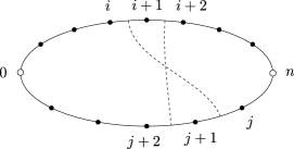
Figure 9.1: Two antiparallel twisted bridges. Compare to Figure 7.1.

It is easy to see that, in addition to ladders whose rungs are straight bridges, antiladders whose rungs are twisted bridges have a leading order contribution.

The skeleton $\Sigma=S(\Gamma)$ of the pairing $\Gamma$ is obtained from $\Gamma$ by the following procedure. A pair of parallel straight bridges is collapsed to form a single straight bridge. A pair of antiparallel twisted bridges is collapsed to form a single twisted bridge. This is repeated until no parallel straight bridges or antiparallel twisted bridges remain. The resulting pairing is the skeleton $\Sigma=S(\Gamma)$; see Figure 9.2.

Figure 9.2: The construction of the tagged skeleton graph.

Thus we see that Lemma 7.3 holds. Moreover, Lemma 7.4 holds, provided that (i) is replaced with

• Each $\Sigma\in\mathscr{S}_{m,m^{\prime}}^{*}$ contains no parallel straight bridges and no antiparallel twisted bridges.

Crucially, Lemma 7.7 remains valid for such tagged skeletons. This can be easily seen using the orbit construction of the proof of Lemma 7.7, combined with (i’).

Next, we associate a factor $D_{\ell}(y,z)$ with each bridge $\sigma\in\Sigma$. If $\sigma$ is straight, this is done exactly as in Section 7.4. If $\sigma$ is twisted, this association follows immediately from the definition of the antiladder. Thus we find that Lemma 7.6 holds. The rest of the analysis in Section 7 carries over almost verbatim; the only required modification is the summation over $2^{\bar{m}}$ tag configurations of the bridges of $\Sigma$. The resulting factor $2^{\bar{m}}$ is immaterial.

Finally, the complete ladder pairing yields (3.1). The complete antiladder is subleading, as its contribution vanishes unless $x=0$.

10 Delocalization: proofs of Theorem 3.3 and Corollary 3.4

In this section we show how to derive Theorem 3.3 from Theorem 3.1, and derive Corollary 3.4 as a consequence.

Proof of Theorem 3.3.

We use an argument due to Chen [9] showing that diffusive motion implies delocalization of the vast majority of eigenvectors.

Recall that $P_{x,\ell}(y)\mathrel{\mathop{:}}=\bm{\mathrm{1}}(\lvert y-x\rvert\geqslant\ell)$ is the characteristic function of the complement (in $\Lambda_{N}$) of the $\ell$-neighborhood of $x$. Also, $\mathfrak{A}_{\varepsilon,\ell}^{\omega}$, defined by

$$\mathfrak{A}^{\omega}_{\varepsilon,\ell}\;=\;\biggl{\{}{\alpha\in\mathfrak{A}\,:\,\sum_{x}\lvert\psi_{\alpha}^{\omega}(x)\rvert\,\lVert P_{x,\ell}\,\psi^{\omega}_{\alpha}\rVert<\varepsilon}\biggr{\}}\,,$$

is the set of eigenvectors localized on a scale $\ell$ up to an error of $\varepsilon$.

By diagonalizing $H^{\omega}$,

$$H^{\omega}\;=\;\sum_{\alpha\in\mathfrak{A}}\lambda^{\omega}_{\alpha}\,|\psi^{\omega}_{\alpha}\rangle\langle\psi^{\omega}_{\alpha}|\,,$$

we have

$$\big{\lVert}P_{x,\ell}\,\mathrm{e}^{-\mathrm{i}tH^{\omega}}\delta_{x}\big{\rVert}^{2} \;=\;\bigg{\lVert}\sum_{\alpha\in\mathfrak{A}}P_{x,\ell}\,\mathrm{e}^{-\mathrm{i}t\lambda_{\alpha}^{\omega}}\,\overline{\psi_{\alpha}^{\omega}(x)}\!\,\,\psi_{\alpha}^{\omega}\bigg{\rVert}^{2}$$

$$\;\leqslant\;\biggl{(}{1+\frac{1}{\zeta}}\biggr{)}\bigg{\lVert}\sum_{\alpha\in\mathfrak{A}_{\varepsilon,\ell}^{\omega}}P_{x,\ell}\,\mathrm{e}^{-\mathrm{i}t\lambda_{\alpha}^{\omega}}\,\overline{\psi_{\alpha}^{\omega}(x)}\!\,\,\psi_{\alpha}^{\omega}\bigg{\rVert}^{2}+(1+\zeta)\bigg{\lVert}\sum_{\alpha\in\mathfrak{A}\setminus\mathfrak{A}_{\varepsilon,\ell}^{\omega}}P_{x,\ell}\,\mathrm{e}^{-\mathrm{i}t\lambda_{\alpha}^{\omega}}\,\overline{\psi_{\alpha}^{\omega}(x)}\!\,\,\psi_{\alpha}^{\omega}\bigg{\rVert}^{2}\,,$$

for any $\zeta>0$. Next, we observe that the norm in the first term may be bounded by 1:

$$\bigg{\lVert}\sum_{\alpha\in\mathfrak{A}_{\varepsilon,\ell}^{\omega}}P_{x,\ell}\,\mathrm{e}^{-\mathrm{i}t\lambda_{\alpha}^{\omega}}\,\overline{\psi_{\alpha}^{\omega}(x)}\!\,\,\psi_{\alpha}^{\omega}\bigg{\rVert}^{2}\;\leqslant\;\bigg{\lVert}\sum_{\alpha\in\mathfrak{A}_{\varepsilon,\ell}^{\omega}}\overline{\psi_{\alpha}^{\omega}(x)}\!\,\,\psi_{\alpha}^{\omega}\bigg{\rVert}^{2}\;=\;\sum_{\alpha\in\mathfrak{A}^{\omega}_{\varepsilon,\ell}}\lvert\psi^{\omega}_{\alpha}(x)\rvert^{2}\;\leqslant\;\sum_{\alpha\in\mathfrak{A}}\lvert\psi^{\omega}_{\alpha}(x)\rvert^{2}\;=\;1\,.$$

Thus we get

$$\big{\lVert}P_{x,\ell}\,\mathrm{e}^{-\mathrm{i}tH^{\omega}}\delta_{x}\big{\rVert}^{2} \;\leqslant\;\biggl{(}{1+\frac{1}{\zeta}}\biggr{)}\bigg{\lVert}\sum_{\alpha\in\mathfrak{A}_{\varepsilon,\ell}^{\omega}}P_{x,\ell}\,\mathrm{e}^{-\mathrm{i}t\lambda_{\alpha}^{\omega}}\,\overline{\psi_{\alpha}^{\omega}(x)}\!\,\,\psi_{\alpha}^{\omega}\bigg{\rVert}+(1+\zeta)\bigg{\lVert}\sum_{\alpha\in\mathfrak{A}\setminus\mathfrak{A}_{\varepsilon,\ell}^{\omega}}\overline{\psi_{\alpha}^{\omega}(x)}\!\,\,\psi_{\alpha}^{\omega}\bigg{\rVert}^{2}$$

$$\;\leqslant\;\biggl{(}{1+\frac{1}{\zeta}}\biggr{)}\sum_{\alpha\in\mathfrak{A}_{\varepsilon,\ell}^{\omega}}\lvert\psi_{\alpha}^{\omega}(x)\rvert\,\lVert P_{x,\ell}\psi_{\alpha}^{\omega}\rVert+(1+\zeta)\sum_{\alpha\in\mathfrak{A}\setminus\mathfrak{A}_{\varepsilon,\ell}^{\omega}}\lvert\psi_{\alpha}^{\omega}(x)\rvert^{2}\,.$$

Averaging over $x\in\Lambda_{N}$ yields

$$\frac{1}{\lvert\mathfrak{A}\rvert}\sum_{x}\big{\lVert}P_{x,\ell}\,\mathrm{e}^{-\mathrm{i}tH^{\omega}}\delta_{x}\big{\rVert}^{2} \;\leqslant\;\biggl{(}{1+\frac{1}{\zeta}}\biggr{)}\frac{1}{\lvert\mathfrak{A}\rvert}\sum_{\alpha\in\mathfrak{A}_{\varepsilon,\ell}^{\omega}}\sum_{x}\lvert\psi_{\alpha}^{\omega}(x)\rvert\,\lVert P_{x,\ell}\psi_{\alpha}^{\omega}\rVert+(1+\zeta)\frac{1}{\lvert\mathfrak{A}\rvert}\sum_{\alpha\in\mathfrak{A}\setminus\mathfrak{A}_{\varepsilon,\ell}^{\omega}}\sum_{x}\lvert\psi_{\alpha}^{\omega}(x)\rvert^{2}\,.$$

$$\;\leqslant\;\biggl{(}{1+\frac{1}{\zeta}}\biggr{)}\varepsilon+(1+\zeta)\frac{\lvert\mathfrak{A}\setminus\mathfrak{A}^{\omega}_{\varepsilon,\ell}\rvert}{\lvert\mathfrak{A}\rvert}\,,$$

by definition of $\mathfrak{A}^{\omega}_{\varepsilon,\ell}$. Therefore

$$\frac{\lvert\mathfrak{A}\setminus\mathfrak{A}^{\omega}_{\varepsilon,\ell}\rvert}{\lvert\mathfrak{A}\rvert}\;\geqslant\;\frac{1}{1+\zeta}\frac{1}{\lvert\mathfrak{A}\rvert}\sum_{x}\big{\lVert}P_{x,\ell}\,\mathrm{e}^{-\mathrm{i}tH^{\omega}}\delta_{x}\big{\rVert}^{2}-\frac{\varepsilon}{\zeta}\,.$$

Taking the expectation yields

$$\mathbb{E}\frac{\lvert\mathfrak{A}\setminus\mathfrak{A}_{\varepsilon,\ell}\rvert}{\lvert\mathfrak{A}\rvert}\;\geqslant\;\frac{1}{1+\zeta}\frac{1}{\lvert\mathfrak{A}\rvert}\mathbb{E}\sum_{x}\big{\lVert}P_{x,\ell}\,\mathrm{e}^{-\mathrm{i}tH}\delta_{x}\big{\rVert}^{2}-\frac{\varepsilon}{\zeta}\;=\;\frac{1}{1+\zeta}\,\mathbb{E}\big{\lVert}P_{0,\ell}\,\mathrm{e}^{-\mathrm{i}tH}\delta_{0}\big{\rVert}^{2}-\frac{\varepsilon}{\zeta}\,,$$ (10.1)

by translation invariance. Note that this estimate holds uniformly in $t$.

Next, pick a continuous function $\varphi(X)$ that is equal to $0$ if $\lvert X\rvert\leqslant 1$ and $1$ if $\lvert X\rvert\geqslant 2$. Recalling that $\varrho(t,x)=\lvert\langle{\delta_{x}}\mspace{2.0mu},{\mathrm{e}^{-\mathrm{i}tH/2}\delta_{0}}\rangle\rvert^{2}$, we find

$$\mathbb{E}\big{\lVert}P_{0,W^{1+d\kappa/2}}\,\mathrm{e}^{-\mathrm{i}tH/2}\delta_{0}\big{\rVert}^{2}\;=\;\sum_{x}\bm{\mathrm{1}}(\lvert x\rvert\geqslant W^{1+d\kappa/2})\,\varrho(t,x)\;\geqslant\;\sum_{x}\varphi\biggl{(}{\frac{x}{W^{1+d\kappa/2}}}\biggr{)}\,\varrho(t,x)\,.$$

Now choose an exponent $\tilde{\kappa}$ satisfying $\kappa<\tilde{\kappa}<1/3$ and set $t=W^{d\tilde{\kappa}}$. Thus,

$$\mathbb{E}\big{\lVert}P_{0,W^{1+d\kappa/2}}\,\mathrm{e}^{-\mathrm{i}W^{d\tilde{\kappa}}H/2}\delta_{0}\big{\rVert}^{2}\;\geqslant\;\sum_{x}\varphi\biggl{(}{W^{d/2(\tilde{\kappa}-\kappa)}\,\frac{x}{W^{1+\tilde{\kappa}d/2}}}\biggr{)}\,\varrho(W^{d\tilde{\kappa}},x)\,.$$

Since we have

$$\lim_{W\to\infty}\varphi\bigl{(}{W^{d/2(\tilde{\kappa}-\kappa)}\,X}\bigr{)}\;=\;1$$

for $X\neq 0$ and $L(1,X)$ is continuous at $X=0$, a simple limiting argument shows that Theorem 3.1 implies

$$\lim_{W\to\infty}\sum_{x}\varphi\biggl{(}{W^{d/2(\tilde{\kappa}-\kappa)}\,\frac{x}{W^{1+d\tilde{\kappa}/2}}}\biggr{)}\,\varrho(W^{d\tilde{\kappa}},x)\;=\;\int\mathrm{d}X\;L(1,X)\;=\;1\,.$$

We have hence proved that

$$\lim_{W\to\infty}\mathbb{E}\big{\lVert}P_{0,W^{1+d\kappa/2}}\,\mathrm{e}^{-\mathrm{i}W^{d\tilde{\kappa}}H/2}\delta_{0}\big{\rVert}^{2}\;=\;1\,,$$

Plugging this into (10.1) yields

$$\liminf_{W\to\infty}\,\mathbb{E}\frac{\lvert\mathfrak{A}\setminus\mathfrak{A}_{\varepsilon,W^{1+d\kappa/2}}\rvert}{\lvert\mathfrak{A}\rvert}\;\geqslant\;\frac{1}{1+\zeta}-\frac{\varepsilon}{\zeta}\,.$$

Setting $\zeta=\sqrt{\varepsilon}$ completes the proof. ∎

Proof of Corollary 3.4.

Pick an intermediate exponent $\widetilde{\kappa}$ satisfying $\kappa<\widetilde{\kappa}<1/3$ and abbreviate

$$\ell\;\mathrel{\mathop{:}}=\;W^{1+d\kappa/2}\,,\qquad\widetilde{\ell}\;\mathrel{\mathop{:}}=\;W^{1+d\widetilde{\kappa}/2}\,.$$

Let $\alpha\in\mathfrak{B}^{\omega}_{\ell}$ and let $u\in\Lambda_{N}$ be as in (3.3). Then we find by Cauchy-Schwarz

$$\biggl{(}{\sum_{x}\lvert\psi^{\omega}_{\alpha}(x)\rvert\,\big{\lVert}P_{x,\widetilde{\ell}}\,\psi^{\omega}_{\alpha}\big{\rVert}}\biggr{)}^{2} \;\leqslant\;\biggl{(}{\sum_{x}\lvert\psi_{\alpha}^{\omega}(x)\rvert^{2}\exp\biggl{[}{\frac{\lvert x-u\rvert}{\ell}}\biggr{]}^{\gamma}}\biggr{)}\biggl{(}{\sum_{x}\exp\biggl{\{}{-\biggl{[}{\frac{\lvert x-u\rvert}{\ell}}\biggr{]}^{\gamma}}\biggr{\}}\big{\lVert}P_{x,\widetilde{\ell}}\,\psi_{\alpha}^{\omega}\big{\rVert}^{2}}\biggr{)}$$

$$\;\leqslant\;K\sum_{\lvert x-y\rvert\geqslant\widetilde{\ell}}\exp\biggl{\{}{-\biggl{[}{\frac{\lvert x-u\rvert}{\ell}}\biggr{]}^{\gamma}}\biggr{\}}\,\lvert\psi_{\alpha}^{\omega}(y)\rvert^{2}$$

$$\;\leqslant\;K\mathrm{e}^{-\delta(\widetilde{\ell}/\ell)^{\gamma}}\sum_{\lvert x-y\rvert\geqslant\widetilde{\ell}}\exp\biggl{\{}{-\biggl{[}{\frac{\lvert x-u\rvert}{\ell}}\biggr{]}^{\gamma}+\delta\biggl{[}{\frac{\lvert x-y\rvert}{\ell}}\biggr{]}^{\gamma}}\biggr{\}}\,\lvert\psi_{\alpha}^{\omega}(y)\rvert^{2}\,,$$

where $\delta>0$ is some small constant to be chosen later. Using $(a+b)^{\gamma}\leqslant(2a)^{\gamma}+(2b)^{\gamma}$ we find

$$\biggl{(}{\sum_{x}\lvert\psi^{\omega}_{\alpha}(x)\rvert\,\big{\lVert}P_{x,\widetilde{\ell}}\,\psi^{\omega}_{\alpha}\big{\rVert}}\biggr{)}^{2}\;\leqslant\;K\mathrm{e}^{-\delta(\widetilde{\ell}/\ell)^{\gamma}}\sum_{x,y}\exp\biggl{\{}{-\biggl{[}{\frac{\lvert x-u\rvert}{\ell}}\biggr{]}^{\gamma}+\delta\biggl{[}{2\frac{\lvert x-u\rvert}{\ell}}\biggr{]}^{\gamma}+\delta\biggl{[}{2\frac{\lvert y-u\rvert}{\ell}}\biggr{]}^{\gamma}}\biggr{\}}\,\lvert\psi_{\alpha}^{\omega}(y)\rvert^{2}\,.$$

Choosing $\delta<2^{-\gamma}$ therefore yields

$$\biggl{(}{\sum_{x}\lvert\psi^{\omega}_{\alpha}(x)\rvert\,\big{\lVert}P_{x,\widetilde{\ell}}\,\psi^{\omega}_{\alpha}\big{\rVert}}\biggr{)}^{2}\;\leqslant\;C\ell^{d}K^{2}\mathrm{e}^{-\delta(\widetilde{\ell}/\ell)^{\gamma}}\;=\mathrel{\mathop{:}}\;\varepsilon_{W}^{2}\,.$$

We have thus proved that $\mathfrak{B}^{\omega}_{\ell}\subset\mathfrak{A}^{\omega}_{\varepsilon_{W},\widetilde{\ell}}$ . Then Corollary 3.4 follows from $\lim_{W\to\infty}\varepsilon_{W}=0$ and Theorem 3.3. ∎

11 Critical pairings

In this section we give an example family of pairings which are critical in the sense that they saturate the 2/3 rule (Lemma 7.7). This implies that extending our results beyond time scales of order $W^{d/3}$ requires either a further resummation of pairings or a more refined classification of graphs in terms of their deviation from the 2/3 rule.

Let $k\geqslant 1$ and consider the skeleton pairing $\Sigma_{k}$ defined in Figure 11.1. It is a critical pairing in the sense that all orbits not containing the vertices $0,m$ consist of $3$ vertices.

Figure 11.1: A critical skeleton pairing $\Sigma_{k}$. The label of each vertex is indicated next to its vertex.

It is easy to see that for $\Sigma_{k}$ we have

$$\bar{m}\;=\;6k+1\,,\qquad L(\Sigma_{k})\;=\;4k+1\,.$$

In particular, the 2/3 rule of Lemma 7.7 is saturated. Moreover, if $\bm{\mathrm{\ell}}_{\Sigma_{k}}$ satisfies $\ell_{\sigma}\geqslant 2$ for all $\sigma\in\Sigma_{k}$ then the associated pairing $\Gamma\mathrel{\mathop{:}}=G_{\bm{\mathrm{\ell}}_{\Sigma_{k}}}(\Sigma_{k})$ has a nonzero contribution $V_{x}(\Gamma)\sim R_{x}(\Gamma)\approx M^{-2k}$ (here, and in the following, we ignore any powers of $W$ with exponent of order one). Indeed, it is easy to check that under the condition $\ell_{\sigma}\geqslant 2$ for all $\sigma$ the above $\Gamma$ satisfies all nonbacktracking conditions. (In fact, it suffices to require that $\ell_{\bar{\sigma}}\geqslant 2$, where $\bar{\sigma}$ is the bridge drawn as a vertical line in Figure 11.1.)

As shown in the Section 7 (see (7.13)), the coefficients $a_{n}(t)$ essentially vanish if $n>(1+o(1))t$. Setting $t=M^{\kappa}$ thus means restricting the summation to $n,n^{\prime}\leqslant M^{\kappa}$.

Assume, to begin with, that we adopt the strategy of Section 7 in estimating the contribution of each graph, i.e. we use the 2/3 rule for each skeleton pairing and the $\ell^{1}$-$\ell^{\infty}$-type estimates from Lemma 7.5 on the edges of the associated multigraph. We show that the sum of the contributions of the skeleton pairings $\Sigma_{k}$ diverges if $\kappa>1/3$. Indeed, noting that $n,n^{\prime}\leqslant M^{\kappa}$ implies $\bar{n}\leqslant M^{\kappa}$, we find that the contribution of all $\Sigma_{k}$’s is

$$\sum_{k=1}^{p/6}\frac{1}{M^{2k}}\sum_{\ell_{1}+\dots+\ell_{6k}=p}1\,,$$ (11.1)

where $p=M^{\kappa}$ and the sum over $\ell_{i}$ is restricted to $\ell_{i}\geqslant 2$ for all $i$. Here we only sum over the pairing of maximal $\bar{n}=p$ (so as to obtain a lower bound), and set $6k+1\approx 6k$. Now (11.1) is equal to

$$\sum_{k=1}^{p/6}\frac{1}{M^{2k}}\binom{p-6k}{6k}\;\sim\;\sum_{k=1}^{p/6}\biggl{(}{\frac{C(M^{\kappa}-6k)}{kM^{1/3}}}\biggr{)}^{6k}\,,$$

which diverges as $W\to\infty$ if $\kappa>1/3$. Hence a control of the error term at time scales $\kappa$ larger than $1/3$ would require further resummation of such critical pairings.

In the estimates of the preceding paragraph we did not make full use of the heat kernel decay associated with each skeleton bridge. For simplicity, the following discussion is restricted to $d=1$ (it may be easily extended to higher dimensions; in fact some estimates are better in higher dimensions). Using Lemma 7.5, we may improve (11.1) to

$$\sum_{k=1}^{p/6}\frac{1}{M^{2k}}\sum_{\ell_{1}+\dots+\ell_{6k}=p}\frac{1}{\sqrt{\ell_{1}\cdots\ell_{2k}}}\,;$$ (11.2)

this is a simple consequence of the heat kernel bound of Lemma 7.5 and the fact that each six-block of $\Sigma_{k}$ contains two bridges in $\Sigma_{k}\setminus(\Sigma_{k})_{T}$ for which we may apply the bound (7.7b) (in which we drop the unimportant second term for simplicity). Now (11.2) is bounded by

$$\sum_{k=1}^{p/6}\frac{1}{M^{2k}}\,p^{k}\binom{p}{4k}\;\sim\;\sum_{k=1}^{p/6}\biggl{(}{\frac{CM^{5\kappa/6}}{k^{2/3}M^{1/3}}}\biggr{)}^{6k}\,,$$ (11.3)

which is summable for $\kappa<2/5$. Note, however, that the factor $k^{-6k}$ from (11.1) has been replaced with the larger factor $k^{-4k}$. Recall that the factor $k^{-6k}$ is used to cancel the combinatorics $\bar{m}!\sim k^{6k}$ arising from the summation over all skeletons. In the present example this small factor is not needed, as the family $\{\Sigma_{k}\}$ is small. It is clear, however, that a systematic application of this approach requires a more refined classification of skeletons in terms of how much they deviate from the 2/3 rule. One expects that the number of skeletons saturating the 2/3 rule is small, and that they are therefore amenable to estimates of type (11.3). Conversely, most of the $\bar{m}!$ skeletons are expected to deviate strongly from the 2/3 rule, so that their greater number is compensated by their small individual contributions.

Finally, we mention that the upper bound (7.7), used in the $\ell^{1}$-$\ell^{\infty}$-type estimates above, neglects the spatial decay of the heat kernel, i.e. that

$$D_{\ell}(x,y)\sim\ell^{-1/2}e^{-(x-y)^{2}/\ell}$$ (11.4)

for $\lvert x-y\rvert\ll N$. Thus a correct lower bound on the contribution of each skeleton graph should have taken into account this additional decay as well. A somewhat lenghtier calculation shows that with the asymptotics (11.4) the estimate (11.2) may be improved to

$$\sum_{k=1}^{p/6}\frac{1}{M^{2k}}\sum_{\ell_{1}+\cdots+\ell_{6k}=p}\;\prod_{j=1}^{k}\frac{1}{\sqrt{\ell^{(j)}_{2}\ell^{(j)}_{4}+\ell^{(j)}_{2}\ell^{(j)}_{6}+\ell^{(j)}_{3}\ell^{(j)}_{4}+\ell^{(j)}_{3}\ell^{(j)}_{6}+\ell^{(j)}_{4}\ell^{(j)}_{5}+\ell^{(j)}_{4}\ell^{(j)}_{6}+\ell^{(j)}_{5}\ell^{(j)}_{6}}}\,,$$

where we abbreviated $\ell^{(j)}_{i}\mathrel{\mathop{:}}=\ell_{6(j-1)+i}$. It is not hard to see that the resulting bound is the same as (11.3), with a smaller constant $C$. In other words, the gain obtained from the spatial decay of the heat kernel is immaterial, and the $\ell^{1}$-$\ell^{\infty}$-estimates cannot be improved.

In conclusion: Our estimates rely on an indiscriminate application of the 2/3 rule to all skeleton pairings; going beyond time scales of order $W^{d/3}$ would require either (i) a refined classification of the skeleton pairings in terms of how much they deviate from the 2/3 rule, combined with a systematic use of the bound (7.7b) on all bridges in $\Sigma\setminus\Sigma_{T}$; or (ii) a further resummation of graphs in order to exploit cancellations. The approach (i) can be expected to reach at most times of order $W^{2/5}$ for $d=1$.

Appendix A Proof of Proposition 8.5

Note first that $F$ is monotone nondecreasing and satisfies $0\leqslant F(\lambda)\leqslant 1$, as follows from (5.4). Hence it is enough to prove (8.5a) for $\lambda\in(0,1)$.

For the following it is convenient to replace $F_{t}$ with $\widetilde{F}_{t}$, defined by

$$\widetilde{F}_{t}(\lambda)\;\mathrel{\mathop{:}}=\;\sum_{n=0}^{[\lambda t]}\lvert\alpha_{n}(t)\rvert^{2}\;=\;F_{t}\biggl{(}{\frac{[t\lambda+1]}{t}}\biggr{)}\,.$$

By Lemma 8.8 we have $F_{t}(\lambda)-\widetilde{F}_{t}(\lambda)=o(1)$ as $t\to\infty$.

Thus let $\lambda\in(0,1)$ be fixed. From (5.2) we find

$$\widetilde{F}_{t}(\lambda)\;=\;\sum_{n=0}^{[\lambda t]}\bigg{\lvert}\frac{2}{\pi}\int_{-1}^{1}\mathrm{d}\xi\,\sqrt{1-\xi^{2}}\,U_{n}(\xi)\,\mathrm{e}^{-\mathrm{i}t\xi}\bigg{\rvert}^{2}\;=\;\sum_{n=0}^{[\lambda t]}\bigg{\lvert}\frac{2}{\pi}\int_{0}^{\pi}\mathrm{d}\theta\;\sin\theta\sin[(n+1)\theta]\,\mathrm{e}^{-\mathrm{i}t\cos\theta}\bigg{\rvert}^{2}\,,$$

where we used (5.1). Thus,

$$\widetilde{F}_{t}(\lambda)\;=\;\frac{1}{\pi^{2}}\int_{0}^{\pi}\mathrm{d}\theta\int_{0}^{\pi}\mathrm{d}\theta^{\prime}\;\sin\theta\,\sin\theta^{\prime}\,\mathrm{e}^{\mathrm{i}t(\cos\theta-\cos\theta^{\prime})}\\ \times\Biggl{[}{\frac{\mathrm{e}^{\mathrm{i}([\lambda t]+1)(\theta+\theta^{\prime})}-1}{\mathrm{e}^{-\mathrm{i}(\theta+\theta^{\prime})}-1}+\frac{\mathrm{e}^{-\mathrm{i}([\lambda t]+1)(\theta+\theta^{\prime})}-1}{\mathrm{e}^{\mathrm{i}(\theta+\theta^{\prime})}-1}-\frac{\mathrm{e}^{\mathrm{i}([\lambda t]+1)(\theta-\theta^{\prime})}-1}{\mathrm{e}^{-\mathrm{i}(\theta-\theta^{\prime})}-1}-\frac{\mathrm{e}^{-\mathrm{i}([\lambda t]+1)(\theta-\theta^{\prime})}-1}{\mathrm{e}^{\mathrm{i}(\theta-\theta^{\prime})}-1}}\Biggr{]}\,,$$ (A.1)

We now claim that the limit $t\to\infty$ of the first two terms of (A.1) vanish by a stationary phase argument. Let us write the first term of (A.1) as $R_{t}^{1}+R_{t}^{2}$, where

$$R_{t}^{1} \;\mathrel{\mathop{:}}=\;\frac{1}{\pi^{2}}\int_{0}^{\pi}\mathrm{d}\theta\int_{0}^{\pi}\mathrm{d}\theta^{\prime}\;\sin\theta\,\sin\theta^{\prime}\,\mathrm{e}^{\mathrm{i}t(\cos\theta-\cos\theta^{\prime})}\frac{\mathrm{e}^{\mathrm{i}([\lambda t]+1)(\theta+\theta^{\prime})}}{\mathrm{e}^{-\mathrm{i}(\theta+\theta^{\prime})}-1}$$

$$\;=\;\frac{1}{\pi^{2}}\int_{0}^{\pi}\mathrm{d}\theta\int_{0}^{\pi}\mathrm{d}\theta^{\prime}\;\frac{\sin\theta\,\sin\theta^{\prime}\,\mathrm{e}^{\mathrm{i}(1-\{\lambda t\})(\theta+\theta^{\prime})}}{\mathrm{e}^{-\mathrm{i}(\theta+\theta^{\prime})}-1}\,\mathrm{e}^{\mathrm{i}t(\cos\theta-\cos\theta^{\prime}+\lambda\theta+\lambda\theta^{\prime})}$$

$$\;=\mathrel{\mathop{:}}\;\int_{0}^{\pi}\mathrm{d}\theta\int_{0}^{\pi}\mathrm{d}\theta^{\prime}\,a_{t}(\theta,\theta^{\prime})\,\mathrm{e}^{\mathrm{i}t\phi(\theta,\theta^{\prime})}\,,$$

where $\{\xi\}\mathrel{\mathop{:}}=\xi-[\xi]\in[0,1)$. One readily finds the bounds

$$\inf_{\theta,\theta^{\prime}\in[0,\pi]}\lvert\nabla\phi(\theta,\theta^{\prime})\rvert\geqslant\lambda\,,\qquad\sup_{\theta,\theta^{\prime}\in[0,\pi]}\lvert\nabla^{2}\phi(\theta,\theta^{\prime})\rvert<\infty\,,\qquad\sup_{t}\sup_{\theta,\theta^{\prime}\in[0,\pi]}\,\lvert\nabla a_{t}(\theta,\theta^{\prime})\rvert\;<\;\infty\,.$$

A standard stationary phase argument therefore yields $\lim_{t\to\infty}R_{t}^{1}=0$.

Similarly, we find

$$R_{t}^{2}\;=\;-\frac{1}{\pi^{2}}\int_{0}^{\pi}\mathrm{d}\theta\int_{0}^{\pi}\mathrm{d}\theta^{\prime}\;\mathrm{e}^{\mathrm{i}t(\cos\theta-\cos\theta^{\prime})}\underbrace{\frac{\sin\theta\,\sin\theta^{\prime}}{\mathrm{e}^{-\mathrm{i}(\theta+\theta^{\prime})}-1}}_{=\mathrel{\mathop{:}}b(\theta,\theta^{\prime})}$$

As above, the functions $b$ and $\nabla b$ are bounded on $[0,\pi]^{2}$. The phase $\cos\theta-\cos\theta^{\prime}$ has four stationary points, $(0,0),(0,\pi),(\pi,0),(\pi,\pi)$, all of them nondegenerate. Therefore a standard stationary phase argument implies that $R^{2}_{t}=O(t^{-1/2})$. (Note that the stationary points lie on the boundary of the integration domain. This is not a problem, however, as the usual stationary phase argument may be applied in combination with the identity $\int_{0}^{\infty}\mathrm{d}x\,\mathrm{e}^{\mathrm{i}tx^{2}}=O(t^{-1/2})$.) Similarly, one shows that the second term of (A.1) vanishes as $t\to\infty$.

Next, as we have just shown, we have

$$\widetilde{F}_{t}(\lambda)\;=\;\widetilde{F}^{0}_{t}(\lambda)+\widetilde{F}^{+}_{t}(\lambda)+\widetilde{F}^{-}_{t}(\lambda)+o(1)$$

for $t\to\infty$, where

$$\widetilde{F}^{0}_{t}(\lambda) \;\mathrel{\mathop{:}}=\;\frac{1}{\pi^{2}}\int_{0}^{\pi}\mathrm{d}\theta\int_{0}^{\pi}\mathrm{d}\theta^{\prime}\;\sin\theta\,\sin\theta^{\prime}\,\mathrm{e}^{\mathrm{i}t(\cos\theta-\cos\theta^{\prime})}\Biggl{[}{\frac{1}{\mathrm{e}^{-\mathrm{i}(\theta-\theta^{\prime})}-1}+\frac{1}{\mathrm{e}^{\mathrm{i}(\theta-\theta^{\prime})}-1}}\Biggr{]}\,,$$

$$\widetilde{F}^{\pm}_{t}(\lambda) \;\mathrel{\mathop{:}}=\;-\frac{1}{\pi^{2}}\int_{0}^{\pi}\mathrm{d}\theta\;\mathcal{P}\int_{0}^{\pi}\mathrm{d}\theta^{\prime}\;\sin\theta\,\sin\theta^{\prime}\,\mathrm{e}^{\mathrm{i}t(\cos\theta-\cos\theta^{\prime})}\frac{\mathrm{e}^{\pm\mathrm{i}([\lambda t]+1)(\theta-\theta^{\prime})}}{\mathrm{e}^{\mp\mathrm{i}(\theta-\theta^{\prime})}-1}\,,$$

where $\mathcal{P}$ denotes principal value. We now show that $\widetilde{F}^{0}_{t}(\lambda)=o(1)$. Indeed, the expression in square brackets in the definition of $\widetilde{F}_{t}^{0}(\lambda)$ is equal to $-1$. Exactly as above we therefore conclude that $\widetilde{F}_{t}^{0}(\lambda)=O(t^{-1/2})$.

Next, let us consider $\widetilde{F}_{t}^{+}(\lambda)$. In a first step, we replace the factor $\frac{1}{\mathrm{e}^{-\mathrm{i}(\theta-\theta^{\prime})}-1}$ with $\frac{1}{-\mathrm{i}(\theta-\theta^{\prime})}$. The error is

$$-\frac{1}{\pi^{2}}\int_{0}^{\pi}\mathrm{d}\theta\;\mathcal{P}\int_{0}^{\pi}\mathrm{d}\theta^{\prime}\;\sin\theta\,\sin\theta^{\prime}\,\mathrm{e}^{\mathrm{i}t(\cos\theta-\cos\theta^{\prime})}\mathrm{e}^{\mathrm{i}([\lambda t]+1)(\theta-\theta^{\prime})}\Biggl{[}{\frac{1}{\mathrm{e}^{-\mathrm{i}(\theta-\theta^{\prime})}-1}-\frac{1}{-\mathrm{i}(\theta-\theta^{\prime})}}\Biggr{]}\,,$$

which vanishes in the limit $t\to\infty$ by the above saddle point argument (the expression in the square brackets is an entire analytic function, and the phase $\cos\theta-\cos\theta^{\prime}+\lambda\theta-\lambda\theta^{\prime}$ has the four nondegenerate saddle points defined by $\sin\theta=\sin\theta^{\prime}=\lambda$).

In a second step, we choose a scale $2/5<\varepsilon<1/2$ and introduce a cutoff in $\lvert\theta-\theta^{\prime}\rvert$ at $t^{-\varepsilon}$. Thus we have

$$\widetilde{F}^{+}_{t}(\lambda)+o(1)\;=\;\frac{1}{\pi^{2}}\int_{0}^{\pi}\mathrm{d}\theta\;\mathcal{P}\int_{0}^{\pi}\mathrm{d}\theta^{\prime}\;\bm{\mathrm{1}}(\lvert\theta-\theta^{\prime}\rvert\leqslant t^{-\varepsilon})\sin\theta\,\sin\theta^{\prime}\,\mathrm{e}^{\mathrm{i}t(\cos\theta-\cos\theta^{\prime})}\frac{\mathrm{e}^{\mathrm{i}([\lambda t]+1)(\theta-\theta^{\prime})}}{\mathrm{i}(\theta-\theta^{\prime})}\,,\\ +\frac{1}{\pi^{2}}\int_{0}^{\pi}\mathrm{d}\theta\int_{0}^{\pi}\mathrm{d}\theta^{\prime}\;\bm{\mathrm{1}}(\lvert\theta-\theta^{\prime}\rvert>t^{-\varepsilon})\sin\theta\,\sin\theta^{\prime}\,\mathrm{e}^{\mathrm{i}t(\cos\theta-\cos\theta^{\prime})}\frac{\mathrm{e}^{\mathrm{i}([\lambda t]+1)(\theta-\theta^{\prime})}}{\mathrm{i}(\theta-\theta^{\prime})}\,,$$ (A.2)

Let us abbreviate $D_{t}\;\mathrel{\mathop{:}}=\;\{(\theta,\theta^{\prime})\in[0,\pi]^{2}\,:\,\lvert\theta-\theta^{\prime}\rvert>t^{-\varepsilon}\}$. The second term on the right-hand side of (A.2) is equal to

$$\frac{1}{\pi^{2}}\int_{D_{t}}\mathrm{d}\theta\,\mathrm{d}\theta^{\prime}\;\mathrm{e}^{\mathrm{i}t(\cos\theta-\cos\theta^{\prime}+\lambda\theta-\lambda\theta^{\prime})}\frac{\sin\theta\,\sin\theta^{\prime}\,\mathrm{e}^{\mathrm{i}(1-\{\lambda t\})(\theta-\theta^{\prime})}}{\mathrm{i}(\theta-\theta^{\prime})}\;=\mathrel{\mathop{:}}\;\int_{D_{t}}\mathrm{d}\theta\,\mathrm{d}\theta^{\prime}\;\mathrm{e}^{\mathrm{i}t\phi(\theta,\theta^{\prime})}\frac{a_{t}(\theta,\theta^{\prime})}{\theta-\theta^{\prime}}\,.$$ (A.3)

In the domain $D_{t}$ the phase $\phi$ has two stationary points defined by $\sin\theta=\sin\theta^{\prime}=\lambda$ and $\theta\neq\theta^{\prime}$. For all $(\theta,\theta^{\prime})$ not in some fixed neighbourhood of these stationary points and satisfying $\lvert\theta-\theta^{\prime}\rvert>t^{-\varepsilon}$, we have the bound

$$\lvert\nabla\phi(\theta,\theta)\rvert\;\geqslant\;Ct^{-\varepsilon}\,,$$

for some constant $C>0$ depending on $\lambda$, and large enough $t$. Thus a standard saddle point analysis shows that (A.3) is of the order $t^{-1/2}+t^{2\varepsilon-1}=o(1)$.

In a third step, we analyse the first term on the right-hand side of (A.2). We introduce the new coordinates

$$u\;=\;\frac{\theta+\theta^{\prime}}{2}\,,\qquad v\;=\;\theta-\theta^{\prime}\,,$$

and write

$$\widetilde{F}_{t}^{+}(\lambda)+o(1) \;=\;\frac{1}{\pi^{2}}\int_{0}^{\pi}\mathrm{d}\theta\;\mathcal{P}\int_{0}^{\pi}\mathrm{d}\theta^{\prime}\;\bm{\mathrm{1}}(\lvert\theta-\theta^{\prime}\rvert\leqslant t^{-\varepsilon})\sin\theta\,\sin\theta^{\prime}\,\mathrm{e}^{\mathrm{i}t(\cos\theta-\cos\theta^{\prime})}\frac{\mathrm{e}^{\mathrm{i}([\lambda t]+1)(\theta-\theta^{\prime})}}{\mathrm{i}(\theta-\theta^{\prime})}$$

$$\;=\;\frac{1}{\pi^{2}}\int_{0}^{\pi}\mathrm{d}u\;\mathcal{P}\int_{-a_{t,u}}^{a_{t,u}}\mathrm{d}v\;\sin\biggl{(}{u+\frac{v}{2}}\biggr{)}\sin\biggl{(}{u-\frac{v}{2}}\biggr{)}\,\mathrm{e}^{\mathrm{i}(1-\{\lambda t\})v}\frac{\mathrm{e}^{\mathrm{i}t(\lambda v-2\sin u\sin\frac{v}{2})}}{\mathrm{i}v}\,,$$

where

$$a_{t,u}\;\mathrel{\mathop{:}}=\;\min\{t^{-\varepsilon},2u,2(\pi-u)\}\,.$$

Now we replace the factor $\mathrm{e}^{\mathrm{i}t(\lambda v-2\sin u\sin\frac{v}{2})}$ with $\mathrm{e}^{\mathrm{i}tv(\lambda-\sin u)}$. The resulting error is

$$R_{t}\;\mathrel{\mathop{:}}=\;\frac{1}{\pi^{2}}\int_{0}^{\pi}\mathrm{d}u\;\mathcal{P}\int_{-a_{t,u}}^{a_{t,u}}\mathrm{d}v\;\sin\biggl{(}{u+\frac{v}{2}}\biggr{)}\sin\biggl{(}{u-\frac{v}{2}}\biggr{)}\,\mathrm{e}^{\mathrm{i}(1-\{\lambda t\})v}\mathrm{e}^{\mathrm{i}tv(\lambda-\sin u)}\frac{\mathrm{e}^{\mathrm{i}t\sin u\,(v-2\sin\frac{v}{2})}-1}{\mathrm{i}v}\,.$$ (A.4)

It is easy to check that, for $v\in[-a_{t,u},a_{t,u}]$, we have

$$\bigg{\lvert}\frac{\mathrm{e}^{\mathrm{i}t\sin u\,(v-2\sin\frac{v}{2})}-1}{\mathrm{i}v}\bigg{\rvert}\;\leqslant\;Ct^{1-\frac{5}{2}\varepsilon}\frac{1}{\sqrt{\lvert v\rvert}}\,.$$

Therefore

$$\lvert R_{t}\rvert\;\leqslant\;C\int_{0}^{\pi}\mathrm{d}u\int_{0}^{2\pi}\mathrm{d}v\;t^{1-\frac{5}{2}\varepsilon}\frac{1}{\sqrt{\lvert v\rvert}}\;=\;o(1)\,.$$

Thus we may write

$$\widetilde{F}_{t}^{+}(\lambda)+o(1)\;=\;\frac{1}{\pi^{2}}\int_{0}^{\pi}\mathrm{d}u\;\underbrace{\mathcal{P}\int_{-a_{t,u}}^{a_{t,u}}\mathrm{d}v\;\sin\biggl{(}{u+\frac{v}{2}}\biggr{)}\sin\biggl{(}{u-\frac{v}{2}}\biggr{)}\,\mathrm{e}^{\mathrm{i}(1-\{\lambda t\})v}\frac{\mathrm{e}^{\mathrm{i}tv(\lambda-\sin u)}}{\mathrm{i}v}}_{=\mathrel{\mathop{:}}I_{t}(u)}\,.$$

In a fourth step, we analyse $I_{t}(u)$ using contour integration. Abbreviate $b\mathrel{\mathop{:}}=\lambda-\sin u$. Let us assume that $u$ satisfies $b\neq 0$. Then, setting $z=\lvert b\rvert tv$, we find

$$I_{t}(u)\;=\;\mathcal{P}\int_{-\lvert b\rvert ta_{t,u}}^{\lvert b\rvert ta_{t,u}}\mathrm{d}z\;\sin\biggl{(}{u+\frac{z}{2\lvert b\rvert t}}\biggr{)}\sin\biggl{(}{u-\frac{z}{2\lvert b\rvert t}}\biggr{)}\,\mathrm{e}^{\mathrm{i}(1-\{\lambda t\})\frac{z}{\lvert b\rvert t}}\frac{\mathrm{e}^{\mathrm{i}z\operatorname{sgn}b}}{\mathrm{i}z}\,.$$

Let us consider the case $b>0$. Using the identity

$$\mathcal{P}\frac{1}{v}\;=\;\mathrm{i}\pi\delta(v)+\frac{1}{v-\mathrm{i}0}$$

and Cauchy’s theorem, we find

$$I_{t}(u)\;=\;\pi\sin^{2}(u)+\int_{\gamma}\mathrm{d}z\;\sin\biggl{(}{u+\frac{z}{2bt}}\biggr{)}\sin\biggl{(}{u-\frac{z}{2bt}}\biggr{)}\,\mathrm{e}^{\mathrm{i}(1-\{\lambda t\})\frac{z}{bt}}\frac{\mathrm{e}^{\mathrm{i}z}}{\mathrm{i}z}\,,$$

where $\gamma$ is the arc $\{bta_{t,u}(\cos\varphi,\sin\varphi)\,:\,\varphi\in[0,\pi]\}$. The absolute value of the integral is bounded by

$$\int_{0}^{\pi}\mathrm{d}\varphi\;\mathrm{e}^{a_{t,u}\sin\varphi}\,\mathrm{e}^{-bta_{t,u}\sin\varphi}\,,$$

which is bounded uniformly in $t$ and $b\neq 0$, and vanishes in the limit $t\to\infty$ for all $b\neq 0$. The case $b<0$ is treated in the same way. In summary, we have, for each $u$ satisfying $\sin u\neq\lambda$, that

$$\lvert I_{t}(u)\rvert\;\leqslant\;C\,,\qquad\lim_{t\to\infty}I_{t}(u)\;=\;\pi\sin^{2}(u)\,\operatorname{sgn}(\lambda-\sin u)\,.$$

Hence by dominated convergence we get

$$\lim_{t\to\infty}\widetilde{F}_{t}^{+}(\lambda)\;=\;\frac{1}{\pi}\int_{0}^{\pi}\mathrm{d}u\;\sin^{2}(u)\,\operatorname{sgn}(\lambda-\sin u)\,.$$

A similar (in fact easier) analysis yields

$$\lim_{t\to\infty}\widetilde{F}_{t}^{-}(\lambda)\;=\;\frac{1}{\pi}\int_{0}^{\pi}\mathrm{d}u\;\sin^{2}(u)\,\operatorname{sgn}(\lambda+\sin u)\,.$$

Therefore we get

$$\lim_{t\to\infty}\widetilde{F}_{t}(\lambda)\;=\;\frac{2}{\pi}\int_{0}^{\pi}\mathrm{d}u\;\sin^{2}(u)\,\bm{\mathrm{1}}(\sin u<\lambda)\;=\;\frac{4}{\pi}\int_{0}^{\lambda}\mathrm{d}\xi\frac{\xi^{2}}{\sqrt{1-\xi^{2}}}\,.$$

This completes the proof of Proposition 8.5.

References

- [1] Abrahams, E., Anderson, P.W., Licciardello, D.C., Ramakrishnan, T.V.: Scaling theory of localization: Absence of quantum diffusion in two dimensions. Phys. Rev. Lett. 42, 673–676.
- [2] Anderson, G.; Zeitouni, O.: A CLT for a band matrix model. Probab. Theory Related Fields 134 (2006), no. 2, 283–338.
- [3] Aizenman, M. and Molchanov, S.: Localization at large disorder and at extreme energies: an elementary derivation, Commun. Math. Phys. 157, 245–278 (1993).
- [4] Aizenman, M., Sims, R., Warzel, S.: Absolutely continuous spectra of quantum tree graphs with weak disorder. Commun. Math. Phys. 264 no. 2, 371–389 (2006).
- [5] Anderson, P.: Absences of diffusion in certain random lattices, Phys. Rev. 109, 1492–1505 (1958).
- [6] Bachmann, S.; De Roeck, W.: From the Anderson model on a strip to the DMPK equation and random matrix theory, J. Stat. Phys. 139, 541–564 (2010).
- [7] Bai, Z.D., Yin, Y.Q.: Limit of the smallest eigenvalue of a large dimensional sample covariance matrix. Ann. Probab. 21 (1993), no. 3, 1275–1294.
- [8] Bourgain, J.: Random lattice Schrödinger operators with decaying potential: some higher dimensional phenomena. Lecture Notes in Mathematics, Vol. 1807, 70–99 (2003).
- [9] Chen, T.: Localization lengths and Boltzmann limit for the Anderson model at small disorders in dimension 3. J. Stat. Phys. 120 (2005), no. 1–2, 279–337.
- [10] Denisov, S.A.: Absolutely continuous spectrum of multidimensional Schrödinger operator. Int. Math. Res. Not. 2004 no. 74, 3963–3982.
- [11] Disertori, M., Pinson, H., Spencer, T.: Density of states for random band matrices. Commun. Math. Phys. 232, 83–124 (2002).
- [12] Disertori, M., Spencer, T.: Anderson localization for a supersymmetric sigma model. Preprint arXiv:0910.3325.
- [13] Disertori, M., Spencer, T., Zirnbauer, M.: Quasi-diffusion in a 3D Supersymmetric Hyperbolic Sigma Model. Preprint arXiv:0901.1652.
- [14] Efetov, K.B.; Supersymmetry in Disorder and Chaos, Cambridge University Press, Cambridge, 1997.
- [15] Elgart, A.: Lifshitz tails and localization in the three-dimensional Anderson model. Duke Math. J. 146 (2009), no. 2, 331–360.
- [16] Erdős, L., Knowles, A.: Quantum diffusion and delocalization for band matrices with general distribution. Preprint arXiv:1005.1838.
- [17] Erdős, L., Péché, G., Ramírez, J., Schlein, B., Yau, H.-T.: Bulk universality for Wigner matrices. Comm. Pure Appl. Math. 63 (2010), no. 7, 895–925.
- [18] Erdős, L., Salmhofer, M., Yau, H.-T.: Quantum diffusion of the random Schrödinger evolution in the scaling limit. Acta Math. 200, no. 2, 211–277 (2008).
- [19] Erdős, L., Salmhofer, M., Yau, H.-T.: Quantum diffusion of the random Schrödinger evolution in the scaling limit II. The recollision diagrams. Commun. Math. Phys. 271, 1–53 (2007).
- [20] Erdős, L., Salmhofer, M., Yau, H.-T.: Quantum diffusion for the Anderson model in scaling limit. Ann. Inst. H. Poincare 8 no. 4, 621–685 (2007).
- [21] Erdős, L., Schlein, B., Yau, H.-T.: Local semicircle law and complete delocalization for Wigner random matrices. Comm. Math. Phys. 287, 641–655 (2009).
- [22] Erdős, L., Schlein, B., Yau, H.-T.: Universality of Random Matrices and Local Relaxation Flow. Preprint arXiv:0907.5605.
- [23] Erdős, L., Schlein, B., Yau, H.-T., Yin, J.: The local relaxation flow approach to universality of the local statistics for random matrices. Preprint arXiv:0911.3687.
- [24] Erdős, L. and Yau, H.-T.: Linear Boltzmann equation as the weak coupling limit of the random Schrödinger equation. Commun. Pure Appl. Math. LIII, 667–735, (2000).
- [25] Erdős, L., Yau, H.-T., Yin, J.: Bulk universality for generalized Wigner matrices. Preprint arXiv:1001.3453.
- [26] Feldheim, O. and Sodin, S.: A universality result for the smallest eigenvalues of certain sample covariance matrices. Preprint arXiv:0812.1961.
- [27] Froese, R., Hasler, D., Spitzer, W.: Transfer matrices, hyperbolic geometry and absolutely continuous spectrum for some discrete Schrödinger operators on graphs. J. Funct. Anal. 230 no. 1, 184–221 (2006).
- [28] Fröhlich, J. and de Roeck, W.: Diffusion of a massive quantum particle coupled to a quasi-free thermal medium in dimension . Preprint arXiv:0906.5178.
- [29] Fröhlich, J. and Spencer, T.: Absence of diffusion in the Anderson tight binding model for large disorder or low energy, Commun. Math. Phys. 88, 151–184 (1983).
- [30] Fröhlich, J., Martinelli, F., Scoppola, E., Spencer, T.: Constructive proof of localization in the Anderson tight binding model. Commun. Math. Phys. 101 no. 1, 21–46 (1985).
- [31] Fyodorov, Y.V. and Mirlin, A.D.: Scaling properties of localization in random band matrices: A -model approach. Phys. Rev. Lett. 67 2405–2409 (1991).
- [32] Gradshteyn, I.S. and Ryzhik, I.M., Tables of integrals, series, and products. Academic Press, New York, 2007.
- [33] Guionnet, A.: Large deviation upper bounds and central limit theorems for band matrices. Ann. Inst. H. Poincaré Probab. Statist 38 , 341–384 (2002).
- [34] Kirsch, W., Krishna, M., Obermeit, J.: Anderson model with decaying randomness: Mobility edge. Math. Z. 235, 421–433 (2000).
- [35] Klein, A.: Absolutely continuous spectrum in the Anderson model on the Bethe lattice. Math. Res. Lett. 1, 399–407 (1994).
- [36] Krasikov, I., Uniform bounds for Bessel functions. J. Appl. Anal. 12, no. 1, 83–91 (2006).
- [37] Mehta, M.L.: Random Matrices. Academic Press, New York, 1991.
- [38] Minami, N.: Local fluctuation of the spectrum of a multidimensional Anderson tight binding model. Comm. Math. Phys. 177, no. 3, 709–725 (1996).
- [39] Rodnianski, I., Schlag, W.: Classical and quantum scattering for a class of long range random potentials. Int. Math. Res. Not. 5, 243–300 (2003).
- [40] Schenker, J.: Eigenvector localization for random band matrices with power law band width. Commun. Math. Phys. 290, 1065–1097 (2009).
- [41] Schlag, W., Shubin, C., Wolff, T.: Frequency concentration and location lengths for the Anderson model at small disorders. J. Anal. Math. 88, 173–220 (2002).
- [42] Sodin, S.: The spectral edge of some random band matrices. Preprint arXiv:0906.4047.
- [43] Spencer, T.: Lifshitz tails and localization. Preprint (1993).
- [44] Spencer, T.: Random banded and sparse matrices (Chapter 23) to appear in “Oxford Handbook of Random Matrix Theory”, edited by G. Akemann, J. Baik and P. Di Francesco.
- [45] Spohn, H.: Derivation of the transport equation for electrons moving through random impurities. J. Statist. Phys. 17, no. 6., 385–412 (1977).
- [46] Tao, T. and Vu, V.: Random matrices: Universality of the local eigenvalue statistics. Preprint arXiv:0906.0510.
- [47] Valkó, B., Virág, B.: Random Schrödinger operators on long boxes, noise explosion and the GOE. Preprint arXiv:0912.0097.
- [48] Wigner, E.: Characteristic vectors of bordered matrices with infinite dimensions. Ann. of Math. 62, 548–564 (1955).