$F_{K}/F_{\pi}$ in full QCD

Abstract:

We determine the ratio $F_{K}/F_{\pi}$ in QCD with $N_{f}=2+1$ flavors of sea quarks, based on a series of lattice calculations with three different couplings, large volumes and a simulated pion mass reaching down to about 190 MeV. We obtain $F_{K}/F_{\pi}=1.192(7)_{stat}(6)_{sys}$ with all the sources of systematic uncertainty under control.

1 Introduction

We determine $F_{K}/F_{\pi}$ in QCD through a series of dynamical lattice calculations such that all the sources of systematic uncertainty are properly taken into account [1]. We use $N_{f}=2+1$ dynamical quarks, with a single quark whose mass is close to the physical strange quark mass ($m_{s}\!\simeq\!m_{s}^{\mathrm{phys}}$), and two degenerate flavours of light quarks heavier than in the real world $u$ and $d$ quarks, but with masses varying trough a range that allows a controlled extrapolation to the physical point. Concerning finite volume effects, the spatial size $L$ is large enough so that the values of $F_{K}/F_{\pi}$in our ensembles can be corrected for small finite-volume effects. We simulate at three different values of $\beta$ to have full control over the continuum extrapolation.

2 Simulation and analysis details

Here we will not give any details about our actions for the gauge and fermion fields, or about the algorithms used for the simulation. The interested reader should consult [2].

To set the scale and adjust the quark masses, we use $aM_{\pi}$, $aM_{K}$ and either $aM_{\Xi}$ or $aM_{\Omega}$ (to estimate the systematics, as we will see). We extrapolate for each value of the lattice spacing the values $aM_{\pi},aM_{K},aM_{\Xi}$ to the point where any two of the ratios agree with the experimental values. We subtract electromagnetic and isosping breaking effects to the experimental values of the masses: we use $M_{\pi}^{\mathrm{phys}}=135\,\mathrm{MeV}$, $M_{K}^{\mathrm{phys}}=495\,\mathrm{MeV}$ and $M_{\Xi}^{\mathrm{phys}}=1318\,\mathrm{MeV}$ with an error of a few MeV, according to [3].

Regarding $m_{ud}$, we have pion masses in the range $190-460\,\mathrm{MeV}$. $F_{K}/F_{\pi}$ is measured with the valence quark masses equal to the sea quark masses (no partial quenching).

The same dataset was successfully used to determine the light hadron spectrum [4].

3 Treatment of the theoretical errors

3.1 Extrapolation to the physical mass point

We simulate with a strange quark mass already close to its physical value, but this is not the case for the light quarks. Thus our values of $F_{K}/F_{\pi}$ need an extrapolation to the physical point. There are three possible guides for this extrapolation: $SU(3)$ chiral perturbation theory, heavy kaon $SU(2)$ chiral perturbation theory, and Taylor fits.

For the case of $SU(3)$ chiral perturbation theory we use the expression for the ratio at NLO as a function of the measured pion and kaon masses. It is important to note here that the apparent convergence of Chiral perturbation theory is a statement that depends both on the observable and the statistical accuracy of the data. With our data, the ratio $F_{K}/F_{\pi}$ is well described by the NLO expression, but this does not mean that NLO expressions can be used in general to describe others quantities (see [5]). The ratio $F_{K}/F_{\pi}$ is probably a benevolent quantity as chiral logs in $F_{\pi}$ and $F_{K}$ cancel in part.

$SU(2)$ chiral perturbation theory [6] and its heavy kaon variant [7] determines the functional dependence of the ratio of decay constants on pion mass. We find that the ratio of NLO expressions from these two references describes well the data in our ensembles.

Having data in the range $190\,\mathrm{MeV}-460\,\,\mathrm{MeV}$, it is natural to consider an expansion about a regular point which encompasses both the lattice results and the physical point [4, 5]. The mass dependence of $F_{K}/F_{\pi}$ in our ensemble and at the physical point is well described by a low order polynomial in $M_{\pi}^{2}$ and $M_{K}^{2}$.

Since all the three frameworks describe well our data, we will use all of them in our analysis, and use the difference between them to estimate the systematic uncertainty.

3.2 Continuum limit

$F_{K}/F_{\pi}$ is an $SU(3)$-flavor breaking ratio, so that cutoff effects must be proportional to $m_{s}-m_{ud}$, that guided by $SU(3)$ chiral perturbation theory we may substitute with $M_{K}^{2}-M_{\pi}^{2}$.

Cutoff effects are both theoretically (they partially cancel in the ratio) and in practice small numerically. In [2] we found that although our action is only formally improved up to order $a$, these small cutoff effects seem to scale like $a^{2}$ up to about 0.16 fm. Even if this is the case we can not exclude the possibility of cutoff effects proportional to $a$. Thus we have considered the following three options compatible with our data: no cutoff effects, and a flavor breaking term proportional to $a$ or $a^{2}$.

3.3 Infinite volume limit

Stable states in a box with periodic boundary conditions have different masses and decay constants than the corresponding states in infinite volume. The difference vanishes exponentially fast with the mass of the lightest state in the box [8]. In our case, masses and decay constants are corrected with terms proportional to $\exp(-M_{\pi}L)$. In our simulations $M_{\pi}L\!\raise 1.29167pt\hbox{$>$\kern-7.5pt\raise-4.73611pt\hbox{$\sim$}}\!4$ making finite volume corrections small. Moreover the sign of leading correction in $F_{\pi}$ and $F_{K}$ is the same, so that they partially cancel in the ratio.

Within chiral perturbation theory, the 1-loop [9, 10] and 2-loop [11] corrections for the pion and kaon decay constants are known, so we have decided to correct the values of our simulations with the 2-loop expression before fitting the data. The 1-loop expression will be used to estimate the systematic uncertainty due to finite volume corrections (see below).

Similarly, we also correct the meson masses [11].

4 Fitting strategy and treatment of theoretical errors

Our goal is to obtain $F_{K}/F_{\pi}$ at the physical point, in the continuum and in infinite volume. To this end we perform a global fit which simultaneously extrapolates or interpolates $M_{\pi}^{2}\to M_{\pi}^{2}|_{\mathrm{phys}}$, $M_{K}^{2}\to M_{K}^{2}|_{\mathrm{phys}}$ and $a\to 0$, after the data have been corrected for very small finite volume effects using the two-loop chiral perturbation theory results discussed above. To assess the various systematic uncertainties associated with our analysis, we perform a large number of alternative fits.

Excited states contribute to the correlators, so to estimate their effect, we choose 18 different time intervals dominated by the ground state. The difference between masses and decay constants coming from different time intervals are used to estimate the uncertainty associated with excited states.

Scale setting systematic uncertainty is estimated by using $M_{\pi}$, $M_{K}$ and either $M_{\Xi}$ or $M_{\Omega}$.

The chiral extrapolation systematic error is estimated in two ways. First we consider two different ranges of pion masses for the fits: $190-350\,\mathrm{MeV}$ and $190-460\,\mathrm{MeV}$. Second, we consider a total of 7 different functional forms to extrapolate to the physical point. 3 of them come from the NLO $SU(3)$ chiral perturbation expression: the ratio of decay constants (cancelling terms proportional to $L_{4}$), a NLO expansion of the ratio and a similar NLO expansion but for the inverse ratio $F_{\pi}/F_{K}$. 2 functional forms come from the $SU(2)$ chiral perturbation theory expression: the expanded ratio of decay constants, and a similar expression but for $F_{\pi}/F_{K}$. The last 2 forms correspond to a Taylor fit for $F_{K}/F_{\pi}$, and a Taylor fit for $F_{\pi}/F_{K}$. It is important to note that the difference between these 7 functional forms provides an estimate of both higher order contributions within a concrete framework (e.g NNLO terms in $SU(3)$ chiral perturbation theory), and systematic bias coming from a particular framework.

As discussed above, cutoff effects are parametrised in three different ways: we consider fits with and without $O(a^{2})$ and $O(a)$ corrections, as described in Sec. 3.2.

Following this procedure we have $18\times 2\times 2\times 7\times 3=1512$ global fits. One of the 1512 fits (corresponding to a specific choice for the time intervals used in fitting the correlators, scale setting, pion mass range, …) can be seen in (Fig. 1a). We emphasize that the $\chi^{2}$ per d.o.f. for our correlated fits are close to one.

Although all these methods seem to describe well our data, not all of them do it in the same way, so we weight with the fit quality the central value of each fit. These 1512 weighted values can be used to construct a distribution, whose median is an estimate of the typical result of our analysis, therefore our desired final result (see fig. 1b). The width of the distribution is a measure of the systematic error of our analysis, thus we take the 16-th/84-th percentiles as an estimate of the systematic error of our computation.

Finite volume effects are treated separately because we know a priori that the two-loop expressions of [11] are the most accurate expressions available and they describe well these effects in our data. To estimate the error associated with the finite volume effects, we repeat the full analysis using the 1 loop expression to correct the ratio $F_{K}/F_{\pi}$ and we also repeat the full analysis correcting only the value of $F_{\pi}$ (this can be seen as an upper bound to the real correction in $F_{K}/F_{\pi}$). The weighted (with the quality of the fit) standard deviation of these three values is used as an estimation of the uncertainty due to finite volume effect, and added to our systematic error by quadratures to produce the final systematic error.

To determine the statistical error, the whole procedure is bootstrapped with 2000 samples, and the standard deviations of the 2000 medians used as our estimate of the statistical error. Our final error is computed as the sum by quadratures of the total systematic and statistical errors.

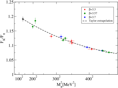
(a) Chiral extrapolation of the lattice data to the physical point for a particular choice of time interval and mass cut ($M_{\pi}<460\,\mathrm{MeV}$ in this case). Here we use a Taylor ansatze with no cutoff effects. The $m_{s}$ dependence has been subtracted to plot the data as a function only of $M_{\pi}$.

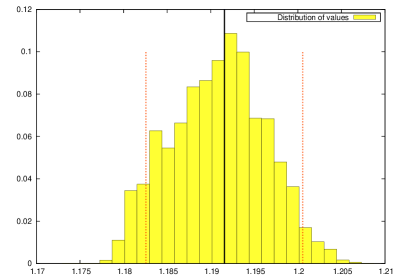
(b) Distribution of values of $F_{K}/F_{\pi}$. The large background distribution (yellow) represents the values of $F_{K}/F_{\pi}$ obtained with different extrapolation formulas, pion mass cuts, parameterization of cutoff effects, time intervals and different methods to set the scale. Also shown is the final error interval (dashed lines) and the final value (black solid vertical line).

Figure 1: And example of mass extrapolation and the distribution of fits used to obtain the final result and systematic error.

5 Results

Our final result for the ratio of decay constants is

$${F_{K}\over F_{\pi}}\bigg{|}_{\mathrm{phys}}=1.192(7)_{\mathrm{stat}}(6)_{\mathrm{syst}}\qquad\mbox{or}\qquad{F_{\pi}\over F_{K}}\bigg{|}_{\mathrm{phys}}=0.839(5)_{\mathrm{stat}}(4)_{\mathrm{syst}}$$ (1)

at the physical point, where all sources of systematic error have been included.

Figure 2a shows our final result compared with the determination of $F_{K}/F_{\pi}$ from other dynamical lattice computations. There are two $N_{f}=2$ computations by JLQCD [13] and ETM [14]. With $2+1$ fermion flavours, we have a number of results obtained using MILC configurations: MILC [3, 15], NPLQCD [16], HPQCD/UKQCD [17] and Aubin et al. [18]. The results by RBC/UKQCD [7] and PACS-CS [19] were also obtained with $N_{f}=2+1$ simulations but with different configurations. It is worth noting that these results show a good overall consistency when one excludes the outlier point of [13].

6 Contributions to the systematic error

Having estimated the total systematic error, it is interesting to decompose it into its individual contributions. To quantify these contributions, we construct a distribution for each of the possible alternative procedures corresponding to the source of theoretical error under investigation. These distributions are constructed by varying over all of the other procedures and weighing the results by the total fit quality. Then, we take the weighted standard deviations of the medians of these distributions as an estimate of the systematic uncertainty associated with the source of error under consideration.

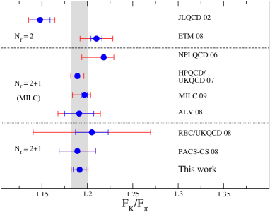
(a) Comparison of recent lattice computations of $F_{K}/F_{\pi}$.

Source of systematic error	error on $F_{K}/F_{\pi}$
Chiral Extrapolation:
- Functional form	$3.3\times 10^{-3}$
- Pion mass range	$3.0\times 10^{-3}$
Continuum extrapolation	$3.3\times 10^{-3}$
Excited states	$1.9\times 10^{-3}$
Scale setting	$1.0\times 10^{-3}$
Finite volume	$6.2\times 10^{-4}$

(b) Breakdown of the total systematic error on $F_{K}/F_{\pi}$ into its various components, in order of decreasing importance.

Figure 2: In the figure, we can see a comparison between our result and recent unquenched computations of $F_{K}/F_{\pi}$. The table shows, in order of importance, the different sources of systematic error.

Table (2b) shows the estimation of the different sources of systematic error in our computation. Even having pion masses down to $190$ MeV, the chiral extrapolation remains the main source of systematic error. This error is broken in two parts by changing the fit range, and using different expressions to extrapolate the data. In the Fig. 3 we can see how fits corresponding to different pion mass cuts, and different functional forms contribute to the final distribution of values. The medians of the small constituent distributions are used to compute the error associated with each source of error, as was mentioned before.

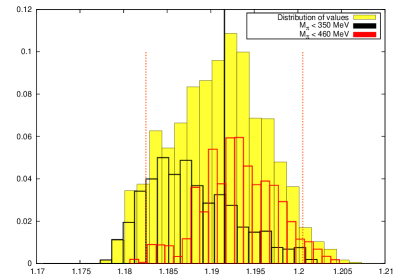
(a) Final distribution of values and the contribution to this corresponding to different pion mass cuts.

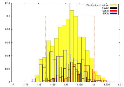
(b) Final distribution of values and the contribution to this corresponding to different functional forms.

Figure 3: Analysis of chiral extrapolation error.

The next source of systematic error in importance are cutoff effects. As was commented earlier, we have three possible parametrizations for the cutoff effects: no cutoff effects at all, a flavor breaking term proportional to $a$, and a flavor breaking term proportional to $a^{2}$. In Fig. 4a the corresponding distributions are shown. In the same way Fig. 5a shows the contributions coming from the two possibilities for setting the scale.

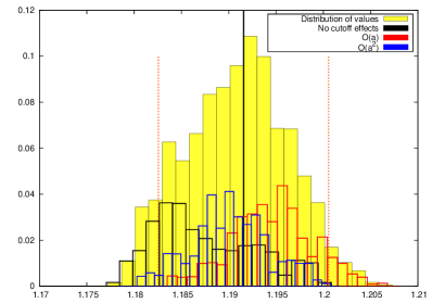
(a) Final distribution of values and the contribution to this corresponding to different cutoff effects.

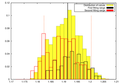
(b) Final distribution of values and the contribution to this corresponding to two different fitting ranges (of the 18 possibilities). The total area of the distributions have been rescaled to make them visible.

Figure 4: Distributions with its contributions coming from different sources of theoretical error.

The two remaining sources of theoretical error deserve a separate comment. First, the contamination with excited states is studied by using a total of 18 different fitting ranges for the correlators, corresponding to $t_{\mathrm{min}}/a=5$ or 6, for $\beta=3.3$; 7, 8 or 9, for $\beta=3.57$; 10, 11 or 12 for $\beta=3.7$. In Fig. 4b we can see the final distribution compared with the distributions corresponding to $t_{\mathrm{min}}/a=5,7,10$ and $t_{\mathrm{min}}/a=6,9,12$. These distributions have been rescaled (so that they add to the total area of our final distribution), to make the small distributions more visible.

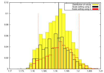
(a) Final distribution of values and the contribution to this corresponding to different scale settings.

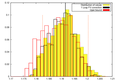
(b) Final distribution of values, compared with the distributions corresponding to a different (1-loop and upper bound) finite volume correction.

Figure 5: Distributions with its contributions coming from different sources of theoretical error.

Second, only the 2-loop finite volume corrections are included in the 1512 fits used to determine the final central value, because we do not want to bias this value with the 1-loop contributions, that are, a priori, less accurate than the 2-loop corrections. To estimate the uncertainty associated with the subtraction of finite volume effects, we repeated the full analysis with 1-loop finite volume corrections and with an upper bound to the correction, computed by including only the 2-loop correction to $F_{\pi}$. Our final distribution of values with these two alternatives are plotted in Fig. 5b. The error associated with the finite volume effects is computed as the weighted (by fit quality) standard deviation of the medians of these three distributions, and added by quadratures to the 68% confidence interval of our final distribution to produce the final systematic error.

One final comment about the procedure to obtain the final systematic error. The addition of different procedures to construct the final distribution only can increase the systematic error. For example in figure (3b) we can clearly see that dropping any of the procedures to extrapolate to the physical point (for example not using $SU(3)$ fits), gives a final value well in our final error band, but a smaller systematic error. This general statement remains true for the other sources of systematic error.

- [1] S. Durr et al., arXiv:1001.4692 [hep-lat].
- [2] S. Dürr et al. [Budapest-Marseille-Wuppertal Collab.], Phys. Rev. D 79, 014501 (2009) [arXiv:0802.2706, hep-lat].
- [3] C. Aubin et al. [MILC Collab.], Phys. Rev. D 70, 114501 (2004) [hep-lat/0407028].
- [4] S. Dürr et al., Science 322, 1224 (2008) [arXiv:0906.3599, hep-lat].
- [5] L. Lellouch, PoS LAT2008, 015 (2009) [arXiv:0902.4545, hep-lat].
- [6] J. Gasser and H. Leutwyler, Annals Phys. 158, 142 (1984).
- [7] C. Allton et al. [RBC/UKQCD Collab.], Phys. Rev. D 78, 114509 (2008) [arXiv:0804.0473, hep-lat].
- [8] M. Lüscher, Commun. Math. Phys. 104, 177 (1986).
- [9] J. Gasser and H. Leutwyler, Phys. Lett. B 184, 83 (1987).
- [10] D. Becirevic and G. Villadoro, Phys. Rev. D 69, 054010 (2004) [hep-lat/0311028].
- [11] G. Colangelo, S. Dürr and C. Haefeli, Nucl. Phys. B 721, 136 (2005) [hep-lat/0503014].
- [12] G. Colangelo and S. Dürr, Eur. Phys. J. C 33, 543 (2004) [hep-lat/0311023].
- [13] S. Aoki et al. [JLQCD Collab.], Phys. Rev. D 68, 054502 (2003) [hep-lat/0212039].
- [14] B. Blossier et al. [ETM Collab.], JHEP 0907, 043 (2009) [arXiv:0904.0954, hep-lat].
- [15] A. Bazavov et al. [MILC Collab.], arXiv:0903.3598 [hep-lat].
- [16] S. R. Beane, P. F. Bedaque, K. Orginos and M. J. Savage [NPLQCD Collab.], Phys. Rev. D 75, 094501 (2007) [hep-lat/0606023].
- [17] E. Follana, C. T. H. Davies, G. P. Lepage and J. Shigemitsu [HPQCD Collab.], Phys. Rev. Lett. 100, 062002 (2008) [arXiv:0706.1726, hep-lat].
- [18] C. Aubin, J. Laiho and R. S. Van de Water, arXiv:0810.4328 [hep-lat].
- [19] S. Aoki et al. [PACS-CS Collab.], Phys. Rev. D 79, 034503 (2009) [arXiv:0807.1661, hep-lat].