Particle Creation from Vacuum by Lorentz Violation

Abstract

It is shown that the vacuum state in presence of Lorentz violation can be followed by a particle-full universe that represents the current status of the universe. In this model the modification in dispersion relation (Lorentz violation) is picked up representing the regime of quantum gravity. The result can be interpreted such that the existence of the particles is an evidence for quantum effects of gravity in the past. It is concluded that only the vacuum state is sufficient to appear the matter fields spontaneously after the process of semi-classical analysis.
PACS: 04.60.-m (Quantum gravity), 04.62.+v (Quantum fields in curved spacetime)

1 Introduction

The big-bang singularity is a prediction of classical general relativity and it must be removed in the final theory. This feature causes concentration of the community on the regimes that the general relativity (gravity) is the dominant field with a very high density. From the other side our knowledge of quantum physics says that in this regime due to enormous density of a field the classical physics is broken and quantum fields become essential. The big-bang and the black-hole are theoretical evidences of quantum gravity, challenge the final theory (at least its gravity sector). Until now different approaches to quantize gravity have grown up e.g. string theory [1] and loop quantum gravity [2]. For such candidates or any given new theory it is very crucial to be falsifiable i.e. it must have some non-trivial accessible predictions, besides the compatibility with their classical counterparts. However due to complexity of quantum gravity it is so hard to calculate any physical prediction comparing to the experiments. To make this comparison possible the test theories are needed which fill the gap between the full theories’ predictions and the experiments. These test theories should possess the structure of the main theories as much as possible. Also there is (are) another layer(s) between the full quantum gravity theories and test theories which is (are) named falsifiable “quantum gravity theory of not everything” [3]. These theories make it possible to transit the great gap between test theories and full theories step by step. As an example noncommutative geometry [4] can be mentioned.

As one of the candidate to model quantum gravity effects is a deviation [3, 5, 6, 7, 8, 9] from the standard dispersion relation among energy and momentum of a particle (Lorentz violation) i.e. $\omega^{2}=k^{2}+m^{2}$ where $\omega$, $k$ and $m$ are energy, momentum’s norm and mass of the particle, respectively. Actually, it is well-known that modification in dispersion relation can appear as a consequence of discretization of space-time on a lattice [3, 10]. Observationally in some cases the modified dispersion relation’s imprints can be found in cosmic ray spectrum [11]. This deviation can be represented by a modification in the dispersion relation such that $\omega^{2}=k^{2}+m^{2}-\alpha^{2}k^{4}$ as a famous example [6]. However, this form of deformation is not a unique choice e.g. introducing a cubic term has been studied in details [7] and a more general form in [8] which contains an observer independent length beside velocity. The coefficient $\alpha^{2}$ is a factor proportional to the minimum length $\ell_{P}$ that makes the semi-classical limit to standard form of dispersion relation trivial due to exiting from quantum gravity regime by taking $\ell_{P}\rightarrow 0$. It is worth mentioning that this prediction is a candidate to go further in the phenomenology of quantum gravity [3, 9]. As mentioned in the above, the phenomenological aspects of quantum gravity is a controversial issue in theoretical physics. Though it is arguable to suppose that the regime of quantum gravity does not make any senses to do some repeatable experiments by humankind but it is believable to accept domination of quantum gravity in early universe. Therefore illustration of this regime may shed some lights on the nature of quantum gravity.

In general to achieve properties of a physical system, knowledge of the dynamical rules besides the correct initial conditions, are needed. For our universe the common believing is that the initial state is a quantum gravitational state due to domination of gravitational field in the very early times. This state has reached to the present state such that the universe contains the particles and also in lack of the quantum effects of gravity. So the question is that how the particle-full universe has risen up from an unknown initial quantum gravitational state? Note that the initial state is an unknown state at least at the present. But as it is usual, with the similar predictions the simpler choice is the better choice. At least in lack of any knowledge about the correct initial state, the simpler choice makes the theory calculable resulting in a general understanding of the theory however it is not complete. The simplest choice for the initial state is the vacuum state, if it does not fall in a trivial prediction. If this simplest choice can predict non-trivial particle-full present status of the universe then the result is very interesting and remarkable. Note that the vacuum state is not only the simplest choice but also is a special choice. This choice makes the proposal of creation from nothing meaningful [12]. The idea of vacuum creation theory has been considered also in different aspects such that under the action of strong fields it is possible to create particle-anti particle plasma system [13, 14]. As mentioned in [14] the time dependent masses can cause particle creation that makes these kind of models comparable to our model which has a time dependent dispersion relation.

In this work, in a toy model we have shown that the above argument can be obtainable. To construct our toy model we pick up the method of particle creation in the context of the quantum field theory in curved space-times [15]. The deformed dispersion relation is used to model the quantum gravitational field i.e. $\omega^{2}=k^{2}+m^{2}-\alpha^{2}k^{4}$. We will propose that the quantum gravity parameter $\alpha^{2}$ has a time dependence such that for very early times be one and vanishing for late times. This evolution behavior is appropriate to study the effects of very early quantum gravity in present time. But it should be mentioned that the function of $\alpha(t)^{2}$ is taken arbitrarily, in lack of any full quantum gravity, such that the equations become solvable analytically.

2 Model

It is generally believed that the notion of particle and as a consequence the notion of vacuum in quantum field theory is not a straightforward manner specially in curved space-times. The crucial part of the definition of states in field theory is the selection of the basis. A field can be expanded due to the appropriate basis $u_{k}(x)$ as follow

$$\varphi(x)=\sum_{k}\left(a_{k}u_{k}(x)+a_{k}^{*}u^{*}_{k}(x)\right)$$ (1)

where $a_{k}$ is a complex number, $x$ and $k$ are four-vectors of position and momentum respectively. In the Minkowskian space-time the choice is trivially $e^{\pm i\vec{k}.\vec{x}}e^{\pm i\omega t}$ such that $\omega^{2}={\vec{k}}^{2}+m^{2}$. The next step is the quantization that is being constructed by transition from complex number coefficients $a_{k}$ to their corresponding operators $\hat{a}_{k}$ and consequently $a_{k}^{*}$ to $\hat{a}^{\dagger}_{k}$, such that the commutation relation $[\hat{a}_{k},\hat{a}_{k^{\prime}}^{\dagger}]=i\hbar\delta_{ij}$ is satisfied by $\hat{a}_{k}$ and $\hat{a}^{\dagger}_{k}$. Due to this relation $\hat{a}_{k}$ and $\hat{a}^{\dagger}_{k}$ can be interpreted as annihilation and creation operators. Finally an $n_{k}$-particle state with momentum $k$, $|n_{k}>$, is being defined by $\hat{N}_{k}=\hat{a}^{\dagger}_{k}\hat{a}_{k}|n_{k}>=n_{k}|n_{k}>$. In the above we reviewed very quickly the structure of definition of states containing particles. As mentioned before the starting point is definition of the appropriate basis that is not trivial for curved space-times [15]. In general cases the symmetries can help in defining the useful basis. This rapid review was needed entering to our model.

In our model we will suppose a Minkowskian space-time as the background but the dispersion relation is different for two sides of the time interval. For the very early times, i.e. for $t\rightarrow-\infty$, it has the form $\omega^{2}=\vec{k}^{2}+m^{2}-\alpha_{0}^{2}\vec{k}^{4}$ where $\alpha_{0}^{2}$ is the Lorentz violation parameter represents the quantum gravity regime in our model. And for very late times, i.e. $t\rightarrow+\infty$, the dispersion relation becomes the standard one, $\omega^{2}=\vec{k}^{2}+m^{2}$. For the late times the natural choice of the basis is $e^{\pm i\vec{k}.\vec{x}}e^{\pm i\omega t}$ where $\omega^{2}=\vec{k}^{2}+m^{2}$. But for the early times these basis are not the suitable ones since the dispersion relation $\omega^{2}=\vec{k}^{2}+m^{2}$ has not any significance in this time region. The natural alternative for this region of time is $e^{\pm i\vec{k}.\vec{x}}e^{\pm i\omega t}$ where $\omega^{2}=\vec{k}^{2}+m^{2}-\alpha_{0}^{2}\vec{k}^{4}$. Since the definitions of basis for these two different regions are not equivalent then the equivalence of the vacuum’s notion for them is not a trivial concept and must restudy again. This feature can cause a deviation from the initial vacuum state and the final vacuum state. This deviation can be interpreted as particle creation during transition from initial to final state. Note that this kind of interpretation is a standard one in quantum field theory in curved space-times [15]. The aim of this paper is to study this concept. To do more, supposing the time evolution of the Lorentz violation parameter is

$$\alpha(t)^{2}=\frac{\alpha_{0}^{2}}{1+e^{t}},$$ (2)

where $\alpha_{0}^{2}$ is the initial value of the Lorentz violation parameter and the general behavior is such that the parameter for the early times and the late times satisfies our above propositions. Otherwise, the form of the function is picked only to make the equations exactly solvable. It must be noted that the origin of this form of time dependence has not been discussed in this work and it seems that this subject belongs to the quantum gravity and specially that branch discussing on the semi-classical limit of quantum gravity. We consider a mass-less scalar field without any loss of generality. To reach to the Klein-Gordon equation it is sufficient to replace $\omega$ and $\vec{k}$ in the dispersion relation by their operator form $-i\partial_{t}$ and $-i\partial_{\vec{x}}$ respectively. So the Klein-Gordon equation becomes

$$\left[\partial^{2}_{t}-\partial^{2}_{\vec{x}}-\alpha(t)^{2}\partial^{4}_{\vec{x}}\right]\varphi(x)=0,$$ (3)

where $x$ is position four-vector. Letting $\varphi(x)\propto e^{i\vec{k}.\vec{x}}T_{k}(t)$ reduces the above equation to

$$\left[\partial^{2}_{t}+k^{2}-\alpha(t)^{2}k^{4}\right]T_{k}(t)=0,$$ (4)

where $k=|\vec{k}|$. The solution of the above second order differential equation is

$$T_{k}(t)=C_{1}e^{-i\left(\sqrt{k^{2}-\alpha_{0}^{2}k^{4}}\right)t}{{}_{2}F_{1}}\left(a,b;c;-e^{t}\right)+C_{2}e^{+i\left(\sqrt{k^{2}-\alpha_{0}^{2}k^{4}}\right)t}{{}_{2}F_{1}}\left(b^{*},a^{*};c^{*};-e^{t}\right)$$ (5)

where ${}_{2}F_{1}$ is the hypergeometric function and

$$a = -ik-i\sqrt{k^{2}-\alpha_{0}^{2}k^{4}}=-i(\omega_{in}+\omega_{out})$$

$$b = +ik-i\sqrt{k^{2}-\alpha_{0}^{2}k^{4}}=-i(\omega_{in}-\omega_{out})$$ (6)

$$c = 1-2i\sqrt{k^{2}-\alpha_{0}^{2}k^{4}}=1-i\hskip 1.42262pt2\omega_{in}$$

To go further we concentrate to the behavior of the both infinite limits. At the first for the very early times, $t\rightarrow-\infty$, the above solution reduces to

$$T_{k}(t\rightarrow-\infty)=C_{1}e^{-i\omega_{in}t}+C_{2}e^{+i\omega_{in}t},$$ (7)

where the identity ${}_{2}F_{1}(a,b;c;0)=1$ for arbitrary $a$, $b$ and $c$ is used [19]. The result is fully in agreement with our expectation since for the very early times the energy is $\omega_{in}=\sqrt{\vec{k}^{2}-\alpha_{0}^{2}\vec{k}^{4}}$. So the first term in (7) can be interpreted as the temporal part of $u_{k}^{in}$ that we will need it in the following calculations. For the second infinite limit, the very late times, the solution becomes more complicated such that

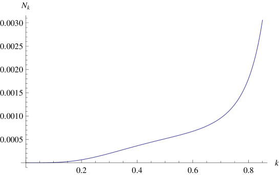
Figure 1: The parameter $\alpha_{0}^{2}=1$ is positive then the plot is not shown for the forbidden region where the $\omega_{in}$ is imaginary (in this case $k>1$ represents forbidden region).

$$T_{k}(t\rightarrow+\infty) = \left[C_{1}\frac{\Gamma(c)\Gamma(a-b)}{\Gamma(a)\Gamma(c-b)}+C_{2}\frac{\Gamma(c^{*})\Gamma(b^{*}-a^{*})}{\Gamma(b^{*})\Gamma(c^{*}-a^{*})}\right]\times e^{-i\omega_{out}\hskip 1.42262ptt}$$ (8)

$$+ \left[C_{1}\frac{\Gamma(c)\Gamma(b-a)}{\Gamma(b)\Gamma(c-a)}+C_{2}\frac{\Gamma(c^{*})\Gamma(a^{*}-b^{*})}{\Gamma(a^{*})\Gamma(c^{*}-b^{*})}\right]\times e^{+i\omega_{out}\hskip 1.42262ptt},$$

where $\Gamma(x)$ is the gamma function. The important point in the above solutions is that for incoming waves $e^{-i\omega_{out}\hskip 1.42262ptt}$ there is a combination of the two terms of the general solutions (5) i.e. $C_{1}$ and $C_{2}$ both appear in the coefficient of the incoming waves and the same is true for the outgoing waves. This means that the vacuum state of the very early universe, $t\rightarrow-\infty$, does not coincide to the vacuum state of the very late times, $t\rightarrow+\infty$. As mentioned before, this interpretation is a standard interpretation in the subject of quantum field theory in curved space-times [15]. For continuing we must calculate the Bogolubov coefficients, $\gamma$ and $\beta$, as the following [15]

$$u_{k}^{in}(x)=\gamma_{k}u_{k}^{out}(x)+\beta_{k}u_{-k}^{out*}(x),$$ (9)

where $x$ is the position four-vector. Note that $u_{k}^{in}$ and $u_{k}^{out}$ are the first terms in relation (1) corresponding to annihilation operator for $in$-region and $out$-region respectively. The non-vanishing $\beta$ results in incoincidence vacua for $in$-region and $out$-region e.g. in our model, the very early times and the very late times respectively. In mathematical language due to relation (7) in our model $u_{k}^{in}(x)$ is the first term in relation (5) times $e^{i\vec{k}.\vec{x}}$ i.e. it contains only the $C_{1}$ factor. But for the $out$-region the result is more complicated such that due to relation (8), $u_{k}^{out}(x)$ equals to a combination of both of terms in (5). The temporal part of the solutions for both of the $in$- and $out$-regions are

$$T_{k}^{in}(t) = \frac{1}{(4\pi\omega_{in})^{\frac{1}{2}}}\hskip 5.69054pte^{-i\omega_{in}t}\hskip 2.84526pt{{}_{2}F_{1}}\left(a,b;c;-e^{t}\right)$$

$$T_{k}^{out}(t) = \frac{(4\pi\omega_{out})^{\frac{1}{2}}}{(4\pi\omega_{in})}\times$$

$$\left(e^{-i\omega_{in}t}\frac{\Gamma(c^{*})\Gamma(a^{*}-b^{*})}{\Gamma(a^{*})\Gamma(c^{*}-b^{*})}\hskip 2.84526pt{{}_{2}F_{1}}(a,b;c;-e^{t})-e^{+i\omega_{in}t}\frac{\Gamma(c)\Gamma(b-a)}{\Gamma(b)\Gamma(c-a)}\hskip 2.84526pt{{}_{2}F_{1}}(b^{*},a^{*};c^{*};-e^{t})\right),$$

such that by taking the limits, the above solutions reduce to the first terms in their counterpart relations (7) and (8). Note that in the above results the prefactors guaranties the normalization of the basis. The second Bogolubov coefficient contributes to show the spectrum of the created particles with respect to the energy i.e. the $|\beta_{k}^{2}|$ is the number of particles with energy $k$, is in the following form

$$N_{k}=\beta_{k}^{2} = \frac{\sinh^{2}(\pi(\omega_{out}-\omega_{in}))}{\sinh(2\pi\omega_{in})\times\sinh(2\pi\omega_{out})}.$$ (11)

The above result can be deduced by some algebra (see the Appendix) from definition of Bogolubov coefficients (9) that has been used for relations (2). The figures show the above number density spectrum for different values of $\alpha_{0}^{2}$. Now let us examine the behavior of the result in well known limits. For $\alpha_{0}^{2}=0$ the expectation is, vanished $N_{k}$ due to no difference between the early and late times. Obviously since in this case $\omega_{in}=\omega_{out}$ it causes vanishing “$\sinh(\pi(\omega_{in}-\omega_{out}))$” in the numerator of the fraction results in vanished $N_{k}$, as expected. Another point is that we have two different choices for $\alpha_{0}^{2}$, a positive one and a negative one. It must be noted that for the positive one, we must restrict the plots to an upper-bound for $k$’s since for the greater values of $k$, $\omega_{in}$ becomes an imaginary number that makes no sense in our conclusions. But for the negative values of $\alpha_{0}^{2}$ the spectrum is valid for all the $k$’s. The figure 1 shows the behavior of the $N_{k}$ with respect to $k$ for a positive $\alpha^{2}_{0}$. In this case as mentioned before, there is a forbidden region due to non-real values of energy $\omega_{in}$. The second figure presents the spectrum of the number of created particles with respect to their energy but for two negative values of $\alpha^{2}_{0}$. It is obvious from the plots that in this case, the maximum of the spectrum is changed by different values of Lorentz violation parameters. The energy, that has the maximum number of created particle, decreasing due to increasing of the absolute value of $\alpha_{0}^{2}$. In this case for smaller value of $\alpha_{0}^{2}$ the plot falls and for $\alpha_{0}^{2}\rightarrow 0$ it coincides to $N_{k}=0$ for all $k$’s, as one expected.

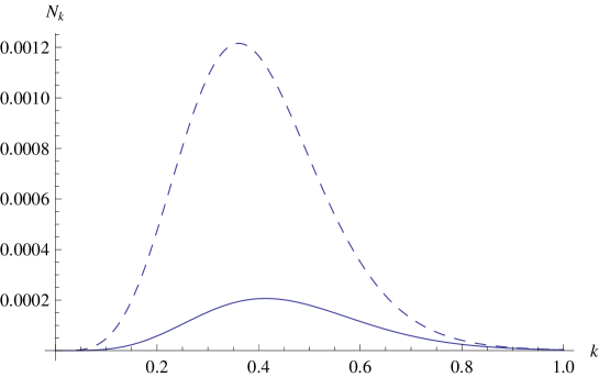
Figure 2: This plot is for two negative $\alpha^{2}_{0}$ with no forbidden region. The solid line presents the spectrum of created particles for $\alpha_{0}^{2}=-1$ and the dashed line for $\alpha_{0}^{2}=-3$.

3 Conclusions

We have studied a toy model to describe the effects of Lorentz violation in particle creation subject [17] in presence of a time dependent deformed dispersion relation. In this paper, we have shown that the existence of Lorentz violation in very early times’ vacuum can result in the existence of particles but in the absence of any Lorentz violation. In the other words we have combined two legitimate individual ingredients, modification of the dispersion relation [6, 7, 8] and time variation of a fundamental parameter [20], to peruse any interesting features. According to above discussions and close relation between Lorentz violation and quantum gravity a suggestion can be introduced that: quantum gravitational vacuum causes a particle-full state in classical gravity. This final state is obtainable by making a semi-classical limitation process. These particle-full states are obtained by taking semi-classical limits of quantum gravitational vacuum. This means particles are only some excitations of quantum gravitational vacuum, that is not an obsolete idea in theoretical physics [21]. In this viewpoint, the particles are the evidences of the past existence of Lorentz violation (or, quantum structure of the geometry (gravity)). The above argument is totally in agreement with some kinds of interpretation of wave function in quantum cosmology such that “probabilistic evolutionary process” interpretation [22]. Since our model is a toy model and far from complete quantum gravity theory, then to see the correctness of our proposal in this paper we need waiting until full quantum gravity theory. This can also shed lights on the origin of the time-dependence of Lorentz violation parameter that is an ambiguity in our model. Finally, it is again worth to mention that in our model only the Lorentz violation is picked up presenting the quantum gravity regime. To discuss more accurate we need to study all the quantum gravitational effects in the presence of the curved background and its dynamics.

At the end it is proper to consider that the origin of the present particles and even the large scale structures can be explained by proposing an inflationary era in the early universe [23]. Maybe it causes to think that the inflationary scenario makes the results of this paper irrelevant. But it is important to note that the inflationary era is not the first stage after the big-bang where quantum gravitational effects are dominant [24]. Our conclusion is that the created particles by Lorentz violation are just before the inflationary era i.e. in contrast to the standard approach in inflationary models the initial state for this era is not vacuum state. In this viewpoint [24] the natural question will be how one can find any traces of these particles after inflationary era in the last scattering surface or even at present time? It seems that at least in our model since the old particles are created by a geometric effect then they show themselves by a geometric feature e.g. gravitational waves [25]. This way of thinking is still open and in this work we did not consider this problem e.g. the effects on CMB temperature fluctuations and etc.

Acknowledgments
I would like to thank H. Firouzjahi, S. Jalalzadeh and M. M. Sheikh-Jabbari for discussions and also anonymous referee for useful comments. This work was supported in part by the Bonyad-e-Nokhbegan grant.

Appendix

In the body of the paper we have used alternatively the following identities among the hypergeometric functions

$$F(a,b;c;z)=F(b,a;c;z) = \frac{\Gamma(c)\Gamma(b-a)}{\Gamma(b)\Gamma(c-a)}(-z)^{-a}F(a,1-c+a;1-b+a;\frac{1}{z})$$

$$+ \frac{\Gamma(c)\Gamma(a-b)}{\Gamma(a)\Gamma(c-b)}(-z)^{-b}F(b,1-c+b;1-a+b;\frac{1}{z})$$

and the following properties for gamma functions

$$\Gamma(1+iy) = iy\Gamma(iy)$$

$$\Gamma(iy)\Gamma(-iy) = \frac{\pi}{y\sinh(\pi y)}$$

where $y$ is a real number.

References

-
[1]
M. B. Green, J. H. Schwarz and E. Witten, “Superstring
Theory”, volumes 1 and 2, Cambridge University Press (1988),
J. Polchinski, “String Theory”, volumes 1 and 2, Cambridge University Press (1998). -
[2]
C. Rovelli, “Quantum Gravity”, Cambridge University Press (2004),
T. Thiemann, “Modern Canonical Quantum General Relativity”, Cambridge University Press (2007). - [3] G. Amelino-Camelia, “Quantum Gravity Phenomenology”, 0806.0339 [gr-qc].
-
[4]
A. Connes, Noncommutative geometry, Academic Press
(1994),
A. Connes, A Short Survey of Noncommutative Geometry, J. Math. Phys. 41, 3832, (2000), hep-th/0003006,
S. Majid, Meaning of Noncommutative Geometry and the Planck-Scale Quantum Group, Lect. Notes Phys. 541, 227, (2000), hep-th/0006166. -
[5]
V. A. Kostelecky and S. Samuel, “Spontaneous breaking of Lorentz symmetry in string theory”, Phys. Rev. D39, 683, (1989),
J. Alfaro, H. Morales-Tecotl and L. Urratia, “Loop quantum gravity and light propagation”, Phys. Rev. D65, 103509, (2002), hep-th/0108061. - [6] T. Jacobson and D. Mattingly, Phys. Rev. D63, 041502, (2001), hep-th/0009052.
- [7] G. Amelino-Camelia, J. Ellis, N. E. Mavromatos, D.V. Nanopoulos and S. Sarkar, “Potential Sensitivity of Gamma-Ray Burster Observations to Wave Dispersion in Vacuo”, Nature 393, 763, (1998), astro-ph/9712103.
- [8] G. Amelino-Camelia, “Relativity in space-times with short-distance structure governed by an observer-independent (Planckian) length scale”, Int. J. Mod. Phys. D11, 35, (2002), gr-qc/0012051.
-
[9]
G. Amelino-Camelia and L. Smolin, “Prospects for constraining quantum gravity dispersion with near term
observations”, Phys. Rev. D80, 084017, (2009), 0906.3731
[hep-th],
G. Amelino-Camelia, L. Smolin and A. Starodubtsev, “Quantum symmetry, the cosmological constant and Planck scale phenomenology”, Class. Quant. Grav. 21, 3095, (2004), hep-th/0306134. - [10] G. ’t Hooft,“Quantization of Point Particles in 2+1 Dimensional Gravity and Space-Time Discreteness”, Class. Quant. Grav. 13, 1023, (1996), gr-qc/9601014.
-
[11]
T. Kifune, “Invariance Violation Extends the Cosmic Ray Horizon?”, Astrophys. J. Lett. L21, 518, (1999), astro-ph/9904164,
R. Aloisio, P. Blasi, P. L. Ghia and A. F. Grillo, “Probing The Structure of Space-Time with Cosmic Rays”, Phys. Rev. D62,053010, (2000), astro-ph/0001258,
G. Amelino-Camelia and T. Piran, “Planck-scale deformation of Lorentz symmetry as a solution to the UHECR and the TeV- paradoxes”, Phys. Rev. D64 ,036005, (2001), astro-ph/0008107,
G. Amelino-Camelia, “Quantum theory’s last challenge”, Nature 408, 661, (2000), gr-qc/0012049,
R. J. Protheroe and H. Meyer, “An infrared background–TeV gamma-ray crisis?”, Phys. Lett. B493, 1, (2000), astro-ph/0005349. - [12] A. Vilenkin, Approaches to quantum cosmology, Phys. Rev. D50, 2581, (1994), gr-qc/9403010 and references therein.
- [13] V. N. Pervushin, V. V. Skokov, A. V. Reichel, S. A. Smolyansky and A. V. Prozorkevich, “The kinetic description of vacuum particle creation in the oscillator representation”, Int. J. Mod. Phys. A20, 5689, (2005), hep-th/0307200.
- [14] A. V. Filatov, A. V. Prozorkevich, S. A. Smolyansky and V. D. Toneev, “Inertial mechanism: dynamical mass as a source of particle creation”, Phys. Part. Nucl. 39, 886, (2008), 0710.0233 [hep-ph].
- [15] N. D. Birrell and P. C. W. Davies, “Quantum Fields in Curved Space”, Cambridge University Press (1982).
-
[16]
S. Carlip, “Quantum Gravity: a Progress Report”, Rept. Prog. Phys. 64, 885,
(2001), gr-qc/0108040,
C. Rovelli, “Graviton propagator from background-independent quantum gravity”, Phys. Rev. Lett. 97, 151301, (2006), gr-qc/0508124. -
[17]
E. Khajeh, N. Khosravi and H. Salehi, “Cosmological Particle Creation in the Presence of Lorentz
Violation”, Phys. Lett. B652, 217, (2007), 0707.3247
[hep-ph],
R. Rashidi, N. Khosravi, E. Khajeh and H. Salehi, “Unruh’s detector in the presence of Lorentz symmetry breaking”, Astrophys Space Sci. 310, 333, (2007), 0706.2767 [hep-th]. - [18] R. Rashidi and H. Salehi, “On the non-existence of micro-causal sector of Lorentz non-invariant quantum field theory on a continuum”, Phys. Lett. B655, 280, (2007).
- [19] M. Abramowitz and I. A. Stegun (editors), “Handbook of Mathematical Functions”, Dover publications (1965).
-
[20]
H. Fritzsch, “The Fundamental Constants in Physics”, Phys. Usp. 52, 359,
(2009), 0902.2989 [hep-ph],
C. Brans and R. H. Dicke, “Mach’s Principle and a Relativistic Theory of Gravitation”, Phys. Rev. 124, 925, (1961). -
[21]
S. O. Bilson-Thompson, F. Markopoulou and L. Smolin,
“Quantum gravity and the standard model”, Class. Quant. Grav.
24, 3975, (2007), hep-th/0603022,
L. Smolin and Y. Wan, “Propagation and interaction of chiral states in quantum gravity”, Nucl. Phys. B796, 331, (2008), 0710.1548 [hep-th]. - [22] N. Khosravi and H. R. Sepangi, “Probabilistic Evolutionary Process: a possible solution to the problem of time in quantum cosmology and creation from nothing”, Phys. Lett. B673, 297, (2009), 0903.1914 [gr-qc].
- [23] S. Weinberg, “Cosmology”, Oxford University Press (2008).
-
[24]
R. Easther, B. R. Greene, W. H. Kinney and G. Shiu,“Imprints of Short Distance Physics On Inflationary
Cosmology”, Phys. Rev. D67, 063508, (2003), hep-th/0110226,
R. H. Brandenberger, “String Gas Cosmology”, 0808.0746 [hep-th]. -
[25]
G. Amelino-Camelia, “An interferometric gravitational wave detector as a quantum-gravity
apparatus”, Nature 398, 216, (1999), gr-qc/9808029,
G. Amelino-Camelia, “Gravity-wave interferometers as probes of a low-energy effective quantum gravity”, Phys. Rev. D62, 024015, (2000), gr-qc/9903080.