A Large-System Analysis of the Imperfect-CSIT Gaussian Broadcast Channel
with a DPC-based Transmission Strategy
Chinmay S. Vaze and Mahesh K. Varanasi
This work was supported in part by NSF Grant CCF-0728955.
The authors are with the Department of Electrical, Computer, and
Energy Engineering, University of Colorado, Boulder, CO 80309-0425
USA (e-mail: vaze, varanasi@colorado.edu).
Abstract
The Gaussian broadcast channel (GBC) with transmit antennas and
single-antenna users is considered for the case in which the
channel state information is obtained at the transmitter via a
finite-rate feedback link of capacity bits per user. The
throughput (i.e., the sum-rate normalized by ) of the GBC is
analyzed in the limit as with . Considering the transmission strategy of zeroforcing dirty
paper coding (ZFDPC), a closed-form expression for the asymptotic
throughput is derived. It is observed that, even under the
finite-rate feedback setting, ZFDPC achieves a significantly higher
throughput than zeroforcing beamforming. Using the asymptotic
throughput expression, the problem of obtaining the number of users
to be selected in order to maximize the throughput is solved.
Index Terms:
broadcast channel, dirty paper coding, inflation factor, zeroforcing
beamforming.
I Introduction
The Gaussian broadcast channel (GBC) has been
intensely researched in recent
years. It is well-known that dirty paper coding (DPC) [1]
achieves the capacity region of the GBC if perfect channel state
information (CSI) is available at the transmitter (CSIT) and the
receivers (CSIR) [2]. However, even though the
assumption of perfect CSIR can be justified, it is unrealistic to
assume the same about CSIT. Moreover, the rate achievable over the
GBC is quite sensitive to the quality of CSIT as has been
demonstrated in [3, 4, 5] (see also
references in [5]). This paper therefore tackles
the important problem of achieving high throughputs using DPC over
the GBC with imperfect CSIT.
It is well known that under perfect CSIT the DPC based transmission
outperforms other known strategies such as zeroforcing beamforming
(ZFBF) [3]. Nevertheless, under imperfect CSIT, it is
the ZFBF strategy that has been intensely researched rather than DPC,
mainly because ZFBF is analytical tractable [4, 6]
and because of a perception that DPC based schemes are either not feasible without perfect CSIT
or, even if feasible, they may be analytically intractable. The main hurdle with DPC is seen to be the
difficulty of designing the inflation factor – a parameter that
can critically affect its performance [1] – without perfect CSIT;
it is even generally believed that the inflation factor cannot be effectively
designed without perfect CSIT [4] implying that DPC
may be overly sensitive to the imperfection in CSIT, thereby rendering it less desirable
than even ZFBF.
Making progress to this end, we recently developed iterative numerical algorithms for the
determination of inflation factor under imperfect CSIT which yield high achievable rates
[7, 8]. Some analytical results were also obtained in the high/low SNR
(signal-to-noise ratio) regime [9, 10]. However,
these results may not always reveal much insight on how DPC works with imperfect CSIT
nor does it shed light on the behavior of DPC at moderate values of SNR.
Moreover, due to the numerical nature of these algorithms, it is almost
impossible to derive analytical results regarding the finite SNR performance of DPC based strategies
or on how they compare with other transmission strategies such as ZFBF. Furthermore,
the algorithms don’t lend themselves to answering important design questions about DPC based schemes –
such as optimizing the sum-rate by selecting (and transmitting to) only a subset of users – other than through a tedious and un-insightful exhaustive search. Recall that the strategy of transmitting to a subset of users
is known to indeed result in a considerable improvement in the sum-rate under
perfect CSIT [3] and for the ZFBF even under imperfect CSIT [6].
To address the above issues, we undertake here a large-system or asymptotic analysis
of the GBC with transmit antennas and single-antenna users (i.e., the GBC of
size/dimension ) in which the CSIT is obtained via a finite-rate
feedback link of capacity bits per user per channel realization (or coherence interval).
In particular, for the transmission strategy of zeroforcing DPC (ZFDPC) [3, 9], we analyze the normalized sum-rate or the throughput
(i.e., the sum-rate divided by ) of the GBC in the limit as with . Such a problem has been
considered before in the special case of perfect CSIT (i.e.,
) in [3] and for the finite-rate feedback
GBC with the simpler transmission strategy of ZFBF in [6].
(1)
(2)
In the large-system limit, the involved random variables converge to
their deterministic limits [11]. Therefore, the
large-system analysis yields a closed-form expression for the
asymptotic throughput (i.e., the throughput in the limit of ), the evaluation of which involves a simple easy-to-compute
numerical integral. Importantly, unlike many works that deal with high SNR
characterizations (c.f., [5] and the references therein)
the asymptotic throughput is obtained as a function of SNR, and hence, it can
provide insights at any finite SNR. It also serves as a simple
semi-analytic tool for the comparison of different transmission
strategies. In particular, contrary to popular belief, we show that even under imperfect
CSIT ZFDPC does indeed achieve a significantly higher throughput than ZFBF.
Furthermore, the asymptotic analysis helps to definitively answer the design question
of optimizing over the number of users to be transmitted to. It is also een that this method when mapped simply to finite dimensions
works quite accurately even for the relatively small values of .
Thus the asymptotic analysis is seen to offer useful insights about
finite-dimensional GBCs as well.
Notations: For a matrix/vector , is its
complex-conjugate transpose. denotes
the circularly symmetric complex normal mean- variance- random
variable (RV), while denotes the chi-square RV of mean
. denotes the vector of
dimension consisting of independent
RVs. For any vector ,
denotes its direction, i.e., , where
denotes the norm of . For a
vector , the perpendicular space of it and the
orthonormal basis vectors spanning the perpendicular space, both,
are denoted by (the meaning is to be understood from the
context). Almost-sure convergence [12] is denoted by
a.s. is an identity matrix. For
RVs and , denotes independence. All logarithms are
to base .
II System Model of GBC
Consider the GBC of size . The received signal at the
user is given by , where is the channel vector of the user,
is the signal transmitted under the
power constraint of , and
is the additive noise. We assume that are independent. Let denote the BF vector for the user and let
. Let be the data symbol to be sent to the
user (’s are independent). Then the total transmitted
signal is given by . Let . We assume perfect
CSIR. Define SNR .
W consider the so-called ‘on-off’ power allocation policy which is that
the transmitter selects a set, denoted , of ‘on’ users
and transmits with equal power to the selected users. In fact, under
perfect CSIT, such a scheme is near optimal. To be precise, the
difference between the asymptotic throughput achieved with the
optimal waterfilling-type power allocation policy [3] and
that obtained using the on-off power policy is negligible.
Hence, we consider here only the on-off power policy.
Under this scheme, if then , where , else . We
let as . Thus, the
asymptotic throughput is obtained as a function of , which
allows us to answer the design problem of optimization over the
fraction of users.
II-AQuantization Scheme
In the limit of large , RVs and , both,
converge to in probability [6, Proposition 1].
Therefore, we find it sufficient, for the present purpose, to
feedback only the channel directions, namely the ’s.
Let denote the number of feedback bits per user. Each user has a
codebook consisting of
-dimensional unit-norm vectors. The vector is
quantized according to the rule: . Denote
by (or simply ) the quantization error
. We further assume
that . We define .
In this paper, we assume the quantization cell approximation (called
the quantization-cell upper-bound (QUB)) [13]. Under
this approximation, we assume ideally that the quantization cell
around each vector of the codebook is a spherical cap of area
times the total surface area of the unit sphere
[13]. It has been shown that this approximation yields
an upper-bound to the performance [13, 14]; and this
upper-bound has been observed to be tight [14]. The tightness
of the bound is a property that depends mainly on how the
quantization error is modeled under the approximation, and not so
much on the channel or the transmission scheme for which the
approximation is being used. Hence, QUB is a reasonable
assumption to make for the present analysis.
Lemma 1
If we write then, under the QUB model, is
isotropically distributed in and is independent of
. Also, a.s.
We consider here an ensemble of codebooks
where is a Haar distributed unitary matrix and
is a given codebook. Then is isotropic. We take the
expectation over the codebooks as well although this is not shown
explicitly in subsequent formulas.
II-BThe Achievable Rate
Assume that the users are encoded according to their natural order.
We focus here on ZFDPC scheme [3, 9]. To obtain
the BF vectors under this scheme, we perform QR-decomposition
[15] of when there is perfect CSIT [3];
i.e., let . The columns of are respectively the BF
vectors of the users. Under finite-rate feedback, we perform the
same procedure with [9]. Note that the BF
vectors are orthogonal and (under finite-rate feedback) , .
We select the auxiliary random variable for the user as
, where is the inflation factor for the
user [1, 8, 9]. Then the achievable
rate for the user is given by equation (1) below (see [8]).
In this scheme, the interference (at user ) due to the users
encoded previously (i.e., users to ) is treated by DPC
whereas that due to the users encoded afterwards (i.e., users
to ) is treated by zeroforcing; hence the name ZFDPC.
Our choice of the inflation factor is stated in equation (2), which is obtained from [8] and
[9]. It is derived by first moving the conditional
expectation in equation (1) inside the
logarithm to obtain an upper-bound on the rate and then maximizing
this upper-bound over the inflation factor.
III Evaluation of the Asymptotic Throughput
We want to evaluate the limit, ,
where each depends on the user index , and hence, on the
normalized user index . In the limit, the normalized
user index would take a value from the continuum, i.e., . We thus anticipate that, as , the above summation would converge to an integral over
and the integrand of which would be the limit of .
To compute the limit, we first need to evaluate the conditional
expectations in (2). We start below with
. Then we
compute and . To this end, note that ; each of these terms is
dealt separately in Subsections III-A to
III-C, respectively. Later, in Subsection
III-D, we find in closed form. Finally,
we evaluate the limit of the terms involved in the denominator of the
argument of the logarithm in (1). We define
. Then .
Lemma 2
.
Proof:
We first prove that . To this end,
consider the unitary matrix ,
where is any arbitrary
unitary matrix. Now, and . Hence, is isotropic in ,
which implies that .
Now, must be of
the form where is positive
semi-definite matrix. We can prove that ,
unitary . This implies that with chosen
such that . Hence .
Now using the decomposition of given in Lemma
1 and noting the fact that we obtain the result.
∎
III-AAnalysis of
1) . Therefore, .
We know a.s. Note that
[11]. Hence, a.s.
Therefore a.s.
2) Now with
. Let us consider . Let ; . Conditioned on ,
is a deterministic direction. Hence, conditioned on ,
. Therefore,
and .
To compute the limit, note that behaves
like , as far as the limit
is concerned. Since the other multiplicative terms remain bounded in
limit, this term converges to zero a.s.
3) One of the cross terms is . Now, ;
.
Since and , the conditional expectation of the cross terms is
zero. Their limit can also be shown to be zero a.s.
III-BAnalysis of
The conditional expectation can be computed using the techniques
developed in Subsection III-A. We directly
state the main result. Note that and
. Then
.
.
To compute the limit, we have .
Thus, are independent random variables. Hence
a.s.
III-CAnalysis of
To compute the conditional expectation, the techniques developed in
Subsection III-A are used. We omit the details
and state the main result:
Since , we get . As in
Subsection III-A, introduce . Then conditioned on
, ; hence unconditionally also, it has the
same distribution. This gives a.s.
III-DComputation of the inflation factor
Let us define . Then we have:
,
, and
We now need . Note that is positive definite
and one of the eigenvectors of or is
while the rest are orthogonal to . Hence, is equal to times the eigenvalue of
corresponding to as the eigenvector. Therefore, we get
(5)
III-EAnalysis of
We have . Further a.s. Let denote the limit
of . Then we can easily obtain the following:
III-FAnalysis of
From equation (5), we can write
for an appropriately chosen
scalar . Then
Let us first analyze the terms and in the above equation. To this end, we have
Using the arguments developed in Subsection III-A Part 2), it can be proved that the terms and converge to zero a.s. Hence, we get
Now, a.s.,
a. s., and
. The limiting value of ,
denoted by , can be easily obtained from the
results of the previous subsection (not shown here explicitly).
Putting together these results, we obtain
Using all the above results, we obtain the asymptotic throughput
as given by equation (III-C).
In the simpler case of perfect CSIT (i.e., as ),
the expression for the asymptotic throughput obtained here reduces
to , which is
same as what one would obtain by specializing the result of
[3] to the ‘on-off’-type power policy.
IV Numerical Results
Let the optimal value of maximizing for the given
value of and be . Let . The asymptotic
throughput for ZFBF is obtained from [6].
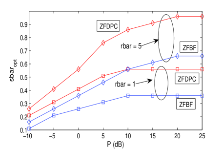
Figure 1: vs. P for and .
In Fig. 1, we plot as
function of for , . It can be seen that for
lower values of , increases with . This
behavior can be understood by noting that if the increased power is
allocated to only a few users, then there would be a ‘logarithmic’
increase in the sum-rate; however, if the power is distributed
across more users then the ‘pre-log’ factor gets improved (i.e.,
more users contribute to the sum-rate). However, increasing
also increases the inter-user interference. Hence, at
higher values of , becomes constant. Next,
increases with because the inter-user
interference reduces with increasing . Finally, note that
for ZFDPC is higher than that for ZFBF. As we would
discuss below, ZFDPC manages the channel gain of the useful signal
and the inter-user interference more efficiently than ZFBF and
hence, corresponding to it turns out to be higher.
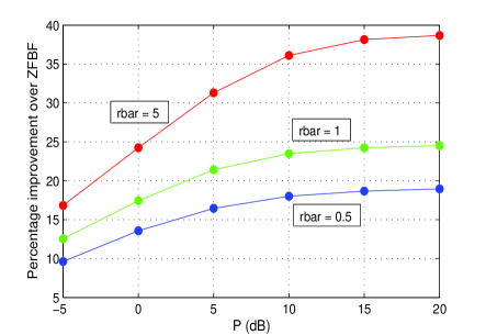
Figure 2: Percentage improvement in the asymptotic throughput
achieved with ZFDPC over ZFBF.
In Fig. 2, we compare the asymptotic
throughput obtained using ZFDPC and ZFBF. The numerical results in
this figure pertain to . Here we plot the percentage
improvement achieved using ZFDPC over ZFBF against for three
values of . We can see that ZFDPC achieves a considerably
higher throughput than ZFBF at all values of and . Note
that even for as low as , the percentage improvement is in
the range of to , which is significant.
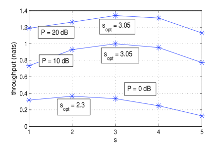
Figure 3: Throughput achieved using ZFDPC vs. for and .
Let us now examine the differences between ZFDPC and ZFBF. Consider
the user. Under ZFDPC, the interference due to users to
is canceled by DPC. This can be accomplished for any given
choice of the BF vectors of users to , as long as the
inflation factor is chosen in the appropriate manner. The BF
vectors are chosen under ZFDPC in such a way that the interference
due to users to gets zeroforced at the user. In
contrast to this, under ZFBF, the BF vectors are selected so as to
zeroforce the interference due to all other users. With this
background, let us now analyze the channel gain of the useful
signal, i.e., the term . Under
ZFDPC, it is proportional the RV
(recall that the other additive terms converge to zero in limit),
whereas under ZFBF, it is proportional to RV [6]. Thus, except for
the user , every other user experiences a stronger channel
under ZFDPC. In other words, DPC (or ZFDPC) manages
the channel gain of the useful signal and the interference together
more effectively than ZFBF. It was known that, due to these
differences, ZFDPC outperforms ZFBF under perfect CSIT [3].
In the light of the results obtained here, we conclude that the same
is true even under imperfect CSIT as well. Lastly, it must be noted that
with ZFBF, the asymptotic throughput is zero when , i.e.,
, . Note that for ZFDPC,
is comparable to . This
behavior can be easily understood by noting the distribution of the
channel gain of the useful signal under two transmission schemes.
Consider now Fig. 3. Here, we plot the
throughput (i.e., the sum-rate normalized by ) for the GBC with
and . We see from the figure that by optimizing over
the number of users, an improvement of about nats can be
obtained (at all values of ), over the simple solution of
transmitting to all users. This improvement is quite
significant, especially at dB and dB. The question
now is how to determine the optimal number of ‘on’ users in the
-dimensional GBC for a given and . Instead of performing
an exhaustive search over , we propose a simple and
computationally efficient approach. First find for
the given and . Then we suggest that for
the -dimensional GBC, select
(rounded to the nearest integer) number of users. In Fig.
3, we see that the maximum value of the
normalized throughput is indeed attained at (rounded to
the nearest integer). We have observed this simple method to work
quite accurately, even for the relatively small values of (
here). Note that the method suggested for the ZFBF in [6]
using their large system analysis
for selecting the number of users is more complicated than the one
suggested here but seems to provide no particular benefit over
this simple approach.
V Conclusion
We provide a large-system analysis of the GBC with finite-rate
feedback and derive a closed-form expression for the asymptotic
throughput achievable using ZFDPC. Using this result, we show that
the DPC-based scheme achieves a significantly higher throughput than
ZFBF. For the first time, DPC is shown to have a better performance,
under imperfect CSIT. Also, using the asymptotic throughput
expression, we address the problem of optimizing over the number of
‘on’ users.
References
[1]
M.Costa, “Writing on dirty paper,” IEEE Trans. Inform. Theory, vol.
29, no. 3, pp. 439–441, May 1983.
[2]
H. Weingarten, Y. Steinberg, and S. Shamai, “The capacity region of
multiple-input multiple-output broadcast channels,” IEEE Trans.
Inform. Theory, vol. 52, no. 9, pp. 3936–3964, Sep. 2006.
[3]
G. Caire and S. Shamai, “On the achievable throughput of a multiantenna
gaussian broadcast channel,” IEEE. Trans. Inform. Theory, vol. 49,
no. 7, pp. 1691–1706, Jul. 2003.
[4]
N. Jindal, “MIMO broadcast channels with finite rate feedback,”
IEEE Trans. Inform. Theory, vol. 52, no. 11, pp. 5045–5060, Nov.
2006.
[5]
C. S. Vaze and M. K. Varanasi, “The degrees of freedom regions of MIMO
broadcast, interference, and cognitive radio channels with no CSIT,”
Sep. 2009, Available Online: http://arxiv.org/abs/0909.5424.
[6]
W. Dai, Y. Liu, B. Rider, and W. Gao, “How many users should be turned on in a
multi-antenna broadcast channel?” IEEE Journal on Sel. Areas of
Comm., vol. 26, Issue 8, pp. 1526–1535, Oct. 2008.
[7]
C. S. Vaze and M. K. Varanasi, “Dirty paper coding for fading channels with
partial transmitter side information,” in Asilomar Conference on
Signals, Systems, and Computers, Pacific Grove, USA, Oct. 2008, pp.
341–345.
[8]
——, “On the achievable rate of the fading dirty paper channel with
imperfect CSIT,” in 43rd Annual Conference on Information
Sciences and Systems, John Hopkins University, Baltimore, USA, Mar. 2009,
pp. 346–351.
[9]
——, “Dirty paper coding for the MIMO gaussian broadcast channels
with imperfect CSIT,” to be submitted to IEEE Trans. Inform.
Theory, 2010, under preparation.
[10]
——, “On the scaling of feedback bits to achieve the full multiplexing gain
over the gaussian broadcast channel using DPC,” in submitted to
IEEE Intern. Symp. Inform. Theory, Jun. 2010.
[11]
A. M. Tulino and S. Verdu, Random Matrix Theory and Wireless
Communications. Foundations and
Trends in Communications and Information Theory, Vol. 1, Issue 1, NOW
publishers.
[12]
A. Papoulis and S. U. Pillai, Probability, Random Variables and
Stochastic Processes. McGraw-Hill
Publishing Company, 2002.
[13]
K. K. Mukkavilli, A. Sabharwal, E. Erkip, and B. Aazhang, “On beamforming with
finite rate feedback in multiple-antenna systems,” IEEE Trans. Inform.
Theory, vol. 49, no. 10, pp. 2562–2579, Oct. 2003.
[14]
T. Yoo, N. Jindal, and A. Goldsmith, “Multi-antenna downlink channels with
limited feedback and user selection,” IEEE Journal on Selected Areas
in Communication, vol. 25, no. 7, pp. 1478–1491, Sep. 2007.
[15]
R. A. Horn and C. R. Johnson, Matrix Analysis. Cambridge Univ. Press, 1985.