Preconditioned fully implicit PDE solvers for monument conservation

Abstract

Mathematical models for the description, in a quantitative way, of the damages induced on the monuments by the action of specific pollutants are often systems of nonlinear, possibly degenerate, parabolic equations. Although some the asymptotic properties of the solutions are known, for a short window of time, one needs a numerical approximation scheme in order to have a quantitative forecast at any time of interest.

In this paper a fully implicit numerical method is proposed, analyzed and numerically tested for parabolic equations of porous media type and on a systems of two PDEs that models the sulfation of marble in monuments. Due to the nonlinear nature of the underlying mathematical model, the use of a fixed point scheme is required and every step implies the solution of large, locally structured, linear systems. A special effort is devoted to the spectral analysis of the relevant matrices and to the design of appropriate iterative or multi-iterative solvers, with special attention to preconditioned Krylov methods and to multigrid procedures. Numerical experiments for the validation of the analysis complement this contribution.

1 Introduction

The problem of monitoring, preserving and, when needed, restoring monuments and works of art has become more and more relevant in recent years for the conservation of our cultural heritage, after the recognition of the negative effects of some pollutants on the monuments. Numerous studies made researchers and restorers more and more aware that gaseous pollutants, atmospheric particulate matter, and some microorganisms can adversely affect the status of our monuments. In order to monitor the cultural heritage and for precisely programming the restoration works, it is of paramount importance to be able to accurately assess the status of each monument. Along these lines, quantitative methods are emerging and making their way into the practice of preservation and restoration. These have the obvious advantage of allowing fair comparison of the state of different monuments, supporting the decision process on what to restore, clean, etc and on the relative urgency of each case.

As an example, consider the “black crusts” that grow on marble surfaces as an effect of sulfation of the carbonate stone that is turned into gypsum when reacting with $\mathrm{SO_{2}}$ in a moist environment. Since urban concentrations of $\mathrm{SO_{2}}$ can be nowadays more than $100$ times higher than the atmospheric basal values, this effect has become very important in the last decades. Sulfation can cause permanent damage to the monuments because gypsum crusts can be easily eroded by rain or (when located in protected areas) can become unaesthetically black including particulate matter from the atmosphere and eventually exfoliate [Hay82, GKPC89, BLTR00].

A better scheduling of cleaning or deeper restoration can be devised if the thickness (and composition) of the crust can be forecast in quantitative way, providing a way to compute and thus predict the time evolution of the crust. The most common quantitative evaluation of the sulfation phenomena that is used in practice consists in assuming that the thickness is directly proportional to the length of time of the exposure to the pollutants, with a proportionality coefficient obtained by fitting data from a large number of monuments [Lip89]. Although this may give an average indication good enough for civil buildings, the uniqueness and cultural importance of a work of art calls for a more detailed analysis, that can take into account the local environment to which the monument is exposed.

A mathematical model of the sulfation of marble based on the chemical reactions involved was developed by Natalini and coworkers [ADDN04, GN05] at IAC-CNR (Rome) and tested against experiments, see [GSNF08].

It is worthwhile to remark that the mathematical model is able to provide new information, which partly contradicts the most common quantitative evaluation methods based on data fitting. In particular (see [GN07]) the asymptotic study of the equations in a one dimensional setting reveals that for large times the thickness of the gypsum crust does not grow proportionally to the elapsed time as in the Lipfert formula, but proportionally to its square root: the speed of growth of the crust is significantly reduced as time goes on. Clearly this means that a complete removal of the crust will speed up the damage and calls for study of optimal strategies for the periodic partial crust removal.

However the asymptotic analysis does not give enough information on what happens for short times and moreover the study is not yet available for complex geometries. For example on a corner stone, $\mathrm{SO_{2}}$ penetrates the marble from two sides: how does the crust grow? Does it get rounded? How much? And, more importantly, what about the fine particulars of decorations or statues? In some cases sulfation caused an almost complete loss of details: can the model predict the thickness of the crust there and allow the scheduling of an optimal conservation strategy? In order to answer the previous questions, we need a numerical method to solve the equations of the model developed by the group in Rome (see [ADDN04]). This is a system of two equations, one of which is nonlinear of parabolic type.

In this paper we generalize and apply novel numerical techniques studied in [SDSC] to integrate for long times nonlinear, possibly degenerate, parabolic equations like those appearing in the model by [ADDN04]. We wish to point out that the techniques developed here have applications that go beyond the aforementioned model. For example, in the area of planned conservation, they could be adapted to numerically investigate the more complete sulfation model described in [AFNT07] and the consolidation model presented in [CGN⁺09].

In the literature, degenerate parabolic equations have been discretized mainly using explicit or semi-implicit methods, thus avoiding to solve the nonlinear equation arising from the elliptic operator. A remarkable class of methods arise directly from the so-called non-linear Chernoff formula [BP72] for time advancement, coupling it with a spatial discretization: for finite differences this was started in [BBR79] and for finite elements by [MNV87]. For example the numerical scheme analysed in [ADDN04] for integrating the sulfation model belongs to the class of semi-implicit methods. More recently, another class related to the relaxation approximation emerged: such numerical procedures exploit high order non-oscillatory methods typical of the discretization of conservation laws and their convergence can be proved making use of semigroup arguments similar to those relevant for proving the Chernoff formula [CNPS07].

In this paper we consider two fully-implicit discretizations in time, thus solving a nonlinear system at each time step. In order to fix ideas, consider the parabolic equation

$$\frac{\partial u}{\partial t}=\nabla\cdot\left(D(u)\nabla u\right),$$ (1)

where $D(u)$ is a non-negative differentiable function and denote with $\mathcal{L}_{D}(u)$ the elliptic operator on the right hand side. Considering a time discretization such that $\mathrm{\Delta}t=t^{n}-t^{n-1}$ and denoting with $U$ the numerical solution, we employ the (first order accurate) Implicit Euler scheme

$$U(t^{n},x)-\mathrm{\Delta}t\mathcal{L}_{D}(U(t^{n},x))=U(t^{n-1},x)$$ (2)

and the (second order accurate) Crank-Nicholson scheme

$$U(t^{n},x)-\frac{\mathrm{\Delta}t}{2}\mathcal{L}_{D}(U(t^{n},x))=U(t^{n-1},x)+\frac{\mathrm{\Delta}t}{2}\mathcal{L}_{D}(U(t^{n-1},x))$$ (3)

(Note that (2) is also known as the Crandall-Liggett formula, after [CL71].)

The computation of $U(t^{n},x)$ with (2) or (3) requires to solve a nonlinear equation whose form is determined by the elliptic operator and the nonlinear function $D(u)$, but the convergence is guaranteed without restrictions on the time step $\mathrm{\Delta}t$. Due to the nonlinear nature of the underlying mathematical model, the use of a fixed point scheme is required and the choice of the faster Newton-like methods implies the solution at every step of large, locally structured (in the sense of Tilli, see [Til98] and [SC06]) linear systems. A special effort was devoted in [SDSC] to the spectral analysis of the relevant matrices and to the design of appropriate iterative or multi-iterative solvers (see [SC93]), with special attention to preconditioned Krylov methods and to multigrid procedures (see [Gre97, Saa03, Hac85, TOS01] and references therein for a general treatment of iterative solvers). In this paper we will argue that those methods can be extended to the case of systems and perform numerical tests on the model of [ADDN04].

The paper is organised as follows. In section 2 we recall the results of [SDSC] on scalar equations, and extend them to the case of a scheme which is second order in time. In Section 3 we introduce the sulfation model, the implicit numerical schemes and the preconditioners for the linear systems. Both sections are complemented by numerical experiments in one and two spatial dimensions. Finally in Section 4 we point out some possible developments of this work.

2 Scalar equations

In this section, we consider the case of a single equation of the porous media type, namely (1), where $D(u)$ is a non-negative differentiable function. The parabolic equation is of degenerate type whenever $D(u)$ vanishes for some values of $u$. For the convergence analysis of our numerical methods, we will require that $D(u)$ is at least continuously differentiable, while the existence of solutions is guaranteed under the milder assumption of continuity [V0́7]. Most applications of the porous media equation involve $D(u)=u^{m}$ for some positive $m$.

For this particular choice, the following self-similar exact solutions have been computed by Barenblatt and Pattle (see [V0́7]):

$$u(t,\mathbf{x})=t^{-\alpha}\left[1-k\left(\frac{|\mathbf{x}|}{t^{\alpha/d}}\right)^{2}\right]_{+}^{\frac{1}{m-1}}\qquad\text{for }t>0,\mathbf{x}\in\mathbb{R}^{d}$$ (4)

where $|\mathbf{x}|=\sqrt{\sum_{1}^{d}x_{i}^{2}}$ and $\alpha=\tfrac{d}{d(m-1)+2}$, $k=\alpha\tfrac{m-1}{2md}$. These solutions are singular for $t=0$, but for $t>0$ represent important reference cases both for the analysis of the solutions of (1) and for numerical tests.

Here, results of [SDSC] on scalar equations are recalled and extended to the case of a scheme which is second order in time. They will be used in section 3, which deals with a system of two equations, since the linear systems arising there include, as a subsystem, those considered in this section.

2.1 Numerical scheme

In order to obtain a numerical scheme for approximating the solutions of (1), we first discretize the time variable with the Crank-Nicholson formula (3), generalising the simpler case of Implicit Euler that was considered in [SDSC]. We point out that searching for high order schemes for equation (1) would seem at first useless, since the exact solution of the equation are in general continuous but not differentiable, so any scheme would converge in theory with order $1$. However, in practice often the exact solution is piecewise regular, allowing an higher order scheme to converge faster than first order and in any case to achieve better errors than (2) at a given spatial resolution, even if the theoretical order of convergence is not reached.

We then complete the discretization by considering the points $x_{k}=a+kh$ in the spatial domain $[a,b]$, where $h=(b-a)/(N+1)$ and $k=0,\ldots,N+1$, and approximating the one-dimensional Laplacian operator with the usual 3-point finite difference formula, i.e.

$$\left.\frac{\partial}{\partial x}\left(D(u)\tfrac{\partial u}{\partial x}\right)\right|_{j}=\frac{D(u)_{j+1/2}\left.\tfrac{\partial u}{\partial x}\right|_{j+1/2}-D(u)_{j-1/2}\left.\tfrac{\partial u}{\partial x}\right|_{j-1/2}}{h}+o(1)\\ =\frac{D(u)_{j+1/2}(u_{j+1}-u_{j})-D(u)_{j-1/2}(u_{j}-u_{j-1})}{h^{2}}+o(1)\\ =\frac{(D(u_{j+1})+D(u_{j}))(u_{j+1}-u_{j})-(D(u_{j})+D(u_{j-1}))(u_{j}-u_{j-1})}{2h^{2}}+o(1)$$ (5)

In order to write down compactly the equations for the numerical scheme, we collect in a vector $\mathbf{u}^{n}$ all the unknown values $u^{n}_{j}=u^{n}(x_{j})$. For example when Dirichlet boundary conditions are considered, since $u_{0}$ and $u_{N+1}$ are known, $\mathbf{u}^{n}$ has $N$ elements, namely $u^{n}_{1},\ldots,u^{n}_{N}$.

We denote by $\mathsf{tridiag}^{N}_{k}[\beta_{k},\alpha_{k},\gamma_{k}]$ a square tridiagonal matrix of order $N$ with entries $\beta_{k}$ on the lower diagonal, $k=2,\cdots,N$, $\alpha_{k}$ on the main diagonal, $k=1,\cdots,N$, and $\gamma_{k}$ on the upper diagonal, $k=1,\cdots,N-1$. We also denote with $\mathsf{diag}^{N}[\alpha_{k}]$ the $N\times{N}$ square diagonal matrix with $\alpha_{k}$ on the $k^{\text{th}}$ row. With this notation, recalling that (3) is a second order approximation,

$$\mathbf{u}^{n}-\mathbf{u}^{n-1}=\frac{1}{2}\frac{\mathrm{\Delta}t}{h^{2}}L_{D(\mathbf{u}^{n})}\mathbf{u}^{n}\frac{1}{2}\frac{\mathrm{\Delta}t}{h^{2}}L_{D(\mathbf{u}^{n-1})}\mathbf{u}^{n-1}+o(\mathrm{\Delta}t^{2}+h^{2})$$ (6)

where

$$L_{D(\mathbf{u})}=\mathsf{tridiag}^{N}_{k}[D_{k-1/2},-D_{k-1/2}-D_{k+1/2},D_{k+1/2}]$$ (7)

and

$$D_{j+1/2}=\frac{D(u_{j+1})+D(u_{j-1})}{2}\,,\;j=0,\ldots,N$$

In two dimensions, on a finite grid composed by the $(N+2)\times(N+2)$ points $\mathbf{x}_{i,j}=a+ih\mathbf{e}_{1}+jh\mathbf{e}_{2}$, where $a$ is the lower left corner of the domain, $h$ the discretization parameter, $\mathbf{e}_{l}$ ($l=1,2$) unit vectors along the coordinate axis and $i,j\in\mathbb{N}$, the matrix $L_{D(\mathbf{u})}$ approximating $\nabla\cdot\left(D(u^{n})\nabla u^{n}\right)$ is pentadiagonal. When considering Dirichlet boundary conditions, adopting the usual lexicographic ordering of the unknowns $u^{n}_{i,j}$, $L_{D(\mathbf{u})}$ is a $N^{2}\times{N^{2}}$ square matrix and nonzero entries can be found only on the main diagonal, on the $1^{\text{st}}$ and $N^{\text{th}}$ upper and lower diagonal.

Finally, we point out that the asymptotic spectral properties of the matrices arising from this discretization ($L_{D}$ in our case), to a large extent, do not depend on the choice of the finite difference formula, but really depend on the Locally Toeplitz structure that in turn arises from operator appearing in the PDE ([SC06]). Thus it should be possible to generalize most of the results of the following sections on linear solvers and preconditioning to other spatial discretizations techniques, including finite element methods.

2.2 Newton method

In order to advance the numerical solution from $\mathbf{u^{n-1}}$ to $\mathbf{u^{n}}$, the nonlinear system of equations (6) must be solved at each timestep. We achieve this, by iterating with the Newton’s method for the function

$$F(\mathbf{u})=\mathbf{u}-\frac{1}{2}\frac{\mathrm{\Delta}t}{h^{2}}L_{D(\mathbf{u})}\mathbf{u}-\frac{1}{2}\frac{\mathrm{\Delta}t}{h^{2}}L_{D(\mathbf{u}^{n-1})}\mathbf{u}^{n-1}-\mathbf{u}^{n-1}$$ (8)

The Jacobian of $F$ is

$$F^{\prime}(\mathbf{u})=X_{N}(\mathbf{u})+Y_{N}(\mathbf{u})$$ (9)

$$X_{N}(\mathbf{u})=I_{N}-\frac{1}{2}\frac{\mathrm{\Delta}t}{h^{2}}L_{D(\mathbf{u})}$$ (10)

$${Y}_{N}(\mathbf{u})=-\frac{1}{2}\frac{\mathrm{\Delta}t}{h^{2}}T_{N}(\mathbf{u})\mathsf{diag}^{N}_{k}(D^{\prime}_{k})$$ (11)

$$T_{N}(\mathbf{u})=\mathsf{tridiag}^{N}_{k}[u_{k-1}-u_{k},u_{k-1}-2u_{k}+u_{k+1},u_{k+1}-u_{k}]$$ (12)

where $T_{N}$ is the same matrix of the first order case (e.g. (12) in one spatial dimension). The only difference in two dimensions is that $T_{N}$ is pentadiagonal.

We observe that the first order scheme based on Implicit Euler gives rise to

$$\widetilde{F}(\mathbf{u})=\mathbf{u}-\frac{\mathrm{\Delta}t}{h^{2}}L_{D(\mathbf{u})}\mathbf{u}-\mathbf{u}^{n-1}$$ (13)

This is the case studied in [SDSC]. Since the Jacobian matrix of $\widetilde{F}$ differs from $F^{\prime}$ only for the missing $\tfrac{1}{2}$ factors in $X_{N}$ and $Y_{N}$, most of the results proved in [SDSC] can be adapted to the present setting. In the following we will thus only sketch the proofs.

Our main result is that the Newton method defined by ${F}$, initialised with $\mathbf{u}^{n,0}=\mathbf{u}^{n-1}$, is convergent under a linear restriction on the timestep. In order to prove it, we need the following estimate for the norm of the inverse of $J$.

Proposition 2.1.

Consider $F(\mathbf{u})$ as defined in (8), where $\mathbf{u}$ is a sampling (at a given time $t$) of a solution $u$ of (1) with $D$ differentiable and having first derivative Lipschitz continuous. If, in addition, $\mathbf{u}$ is differentiable with Lipschitz continuous first derivative, we have that

$$\left\|F^{\prime}(\mathbf{u})^{-1}\right\|_{\infty}\leq C_{1}$$ (14)

for $h$ sufficiently small and under the additional assumption that $\mathrm{\Delta}t\leq C_{\infty}h$ for some $C_{\infty}>0$ that does not depend on $h$.

Proof.

$F^{\prime}(\mathbf{u})$ differs from $\widetilde{F}^{\prime}(\mathbf{u})$ for $\widetilde{F}$ defined in (13) only by factors $\tfrac{1}{2}$ appearing before any $D_{k+1/2}$ term. Since these terms are discarded in the estimates for the proof of the analogous result for $F$, the same proof is valid here. See [SDSC] for the details. ∎

The following result is a classical tool (see [OR70]) for handling the global convergence of the Newton procedure.

Theorem 2.2 (Kantorovich).

Consider the Newton method for approximating the zero of a vector function $F(\mathbf{u})$, starting from the initial approximation $\mathbf{u}^{(0)}$. Under the assumptions that

$$\|\left[F^{\prime}(\mathbf{u}^{(0)})\right]^{-1}\|\leq\beta\,,$$ (15a)

$$\|\left[F^{\prime}(\mathbf{u}^{(0)})\right]^{-1}F(\mathbf{u}^{(0)})\|\leq\eta\,,$$ (15b)

$$\|F^{\prime}(\mathbf{u})-F^{\prime}(\mathbf{v})\|\leq\gamma\|\mathbf{u}-\mathbf{v}\|\,,$$ (15c)

and that

$$\beta\eta\gamma<\frac{1}{2}\,,$$ (16)

the method is convergent and, in addition, the stationary point of the iterations lies in the ball with centre $\mathbf{u}^{(0)}$ and radius

$$\frac{1-\sqrt{1-2\beta\eta\gamma}}{\beta\gamma}.$$

Theorem 2.3.

The Newton method for $\widetilde{F}(\mathbf{u})$ defined in (8) for computing $\mathbf{u}^{n}$ is convergent when initialised with the solution at the previous timestep (i.e. $\mathbf{u}^{n,0}=\mathbf{u}^{n-1}$) and for $\mathrm{\Delta}t\leq Ch$, for a positive constant $C$ independent of $h$.

Proof.

The proof of the same statement for $F$ as given in [SDSC09] can be easily adapted to the present case. The technique is to first establish estimates (15) as follows:

• $\beta\leq C_{1}$ if $\mathrm{\Delta}t\leq C_{\infty}h$ by Proposition 2.1

• $\eta\leq\beta C_{2}\mathrm{\Delta}t$ by first applying Proposition 2.1 again and then estimating

  $$\left\|\widetilde{F}(\mathbf{u}^{n,0})\right\|_{\infty}=\left\|\widetilde{F}(\mathbf{u}^{n-1})\right\|_{\infty}=\mathrm{\Delta}t\left\|L_{D(\mathbf{u}^{n-1})}\mathbf{u}^{n-1}\right\|_{\infty}=O(\mathrm{\Delta}t)$$

• $\gamma\leq 8\|D^{\prime}\|_{\infty}\tfrac{\mathrm{\Delta}t}{h^{2}}$ by direct computation as in [SDSC].

This implies that condition (16) can be satisfied when choosing $\mathrm{\Delta}t\leq Ch$ for a sufficiently small positive constant $C$ that is independent of $h$. ∎

Remark 2.4.

Setting the initial guess with the average between $\mathbf{u}^{n-1}$ and the value given by an Explicit Euler step, like

$$\mathbf{u}^{n,0}=\mathbf{u}^{n-1}+\frac{1}{2}\frac{\mathrm{\Delta}t}{h^{2}}L_{D(\mathbf{u}^{n-1})}\mathbf{u}^{n-1}$$

does not change the convergence ratio, but in practice one needs less iterations to reach a given tollerance.

2.3 Iterative methods for the linear system

Of course the Jacobian matrix $F^{\prime}(\mathbf{u}^{n,(s)})$ is not explicitly inverted at each Newton step, but instead we compute the $(s+1)^{\text{th}}$ Newton iterate by first solving the linear system

$$F^{\prime}(\mathbf{u}^{n,(s)})\mathbf{v}^{(s)}=F(\mathbf{u}^{n,(s)})$$

for $\mathbf{v}^{(s)}$ and then setting

$$\mathbf{u}^{n,(s+1)}=\mathbf{u}^{n,(s)}+\mathbf{v}^{(s)}$$

The matrix $A_{N}=F^{\prime}(\mathbf{u}^{n,(s)})$ is a square tridiagonal (respectively pentadiagonal) $N\times{N}$ (respectively $N^{2}\times{N^{2}}$) matrix when the domain is one (respectively two) dimensional. Its spectral properties are crucial in choosing an appropriate solver for the linear system. Given the large dimension of the system, we aim at an iterative method with an optimal preconditioner, so that we can compute $\mathbf{v}^{(s)}$, on average, in a finite number of iterations.

Moreover $A_{N}$ differs from $\widetilde{F}^{\prime}$ only by the factors $\tfrac{1}{2}$ that were missing in the matrices studied in [SDSC]. It can thus be shown that $A_{N}$ is not symmetric, but it is dominated by its symmetric part $(A_{N}+A_{N}^{\mathsf{T}})/2$, which is in turn essentially a weighted laplacian. Rather detailed information on the spectrum of $A$ can be gained via the theory of Locally Toeplitz Sequences of [Til98]. In particular, when $\mathrm{\Delta}t$ is chosen proportional to $h$, the sequence of $N\times N$ matrices $\{hA_{N}\}$ obtained for increasing number of grid points is Locally Toeplitz (in the sense of [Til98]) with respect to the pair of functions $\left(D(u(x)),2-2\cos(s)\right)$ defined on $[a,b]\times[0,2\pi]$. Hence (see [SDSC]) we can expect the GMRES method, which is picked due to the asymmetry of $A_{N}$ as the main iterative solver, to converge in $O(\sqrt{N})$ iterations.

In order to study a preconditioning strategy, first observe that the sequence $\{X_{N}\}$ of the symmetric parts of $A_{N}$ is also Locally Toeplitz with respect to the same generating functions. Next recall that any Locally Toeplitz sequence is also Generalized Locally Toeplitz, a class which is an closed under inversion, defined in [SC06]. Hence both sequences are also Generalized Locally Toeplitz sequences and $\{X_{N}^{-1}A_{N}\}$ is Generalized Locally Toeplitz with generating function $1$ and thus the singular values are weakly clustered at the point $1$. This is enough to guarantee the superlinear convergence of the preconditioned GMRES methods, but in [SDSC] we also show that the clustering is strong, proving that $X_{N}$ is an optimal preconditioner for solving a linear system with matrix $\{A_{N}\}$ with GMRES, i.e. a given error reduction is reached within a number of iterations which is independent on the problem size $N$.

Unfortunately there is not a fast direct solver for $X_{N}$, so we resort to a Multigrid Method (MGM) with a Galerkin approach. The MGM [TOS01] consist in constructing a solution of a linear system by composing the action of simple iterative schemes (like Jacobi or Gauss-Seidel), that are run on the original system and on smaller systems derived from the first one and called coarse grid approximations.

More precisely, in order to solve a linear system $X\mathbf{u}=\mathbf{b}$ in $\mathbb{R}^{m}$, one considers a finite sequence of integers $m_{0}=m>m_{1}>m_{2}>\dots>m_{\ell}>0$ and full-rank matrices $P^{(i)}_{(i+1)}\in\mathbb{R}^{m_{i+1}\times m_{i}}$ (called projections) and defines the V-cycle method as

$$\mathbf{u^{k+1}}=MGM(0,\mathbf{u}^{k},\mathbf{b})$$

with MGM defined recursively as follows:

$$\begin{array}[]{c}\mathbf{u}_{i}^{({\rm out})}:=MGM(i,\mathbf{u}^{({\rm in})}_{i},\mathbf{b}_{i})\\ \hline\cr\\[-7.11317pt] \begin{array}[]{l@{}ll|l@{}l}\text{If (}i=l\text{) }&\lx@intercol\text{Then Solve(}A_{\ell}\mathbf{u}^{({\rm out})}_{\ell}=\mathbf{b}_{\ell}\text{)}\hfil\lx@intercol\\ &\text{Else}&\bf{1}&\widetilde{\mathbf{u}}_{i}&:=S^{\nu}_{i}\big{(}\mathbf{u}^{({\rm in})}_{i}\big{)}\\ &&\bf{2}&\mathbf{r}_{i}&:=A_{i}\widetilde{\mathbf{u}}_{i}-\mathbf{b}_{i}\\ &&\bf{3}&\mathbf{b}_{i+1}&:=P^{(i)}_{(i+1)}\mathbf{r}_{i}\\ &&\bf{4}&A_{(i+1)}&:=P^{(i)}_{(i+1)}A_{(i)}{(P^{(i)}_{(i+1)})}^{\mathsf{T}}\\ &&\bf{5}&\mathbf{y}_{i+1}&:=MGM(i+1,\mathbf{0}_{n_{i+1}},\mathbf{b}_{i+1})\\ &&\bf{6}&\mathbf{u}^{({\rm out})}_{i}&:=\widetilde{\mathbf{u}}_{i}-{(P^{\,i}_{i+1})}^{\mathsf{T}}\mathbf{y}_{i+1}\\ \end{array}\end{array}$$

Step 1 performs some ($\nu$) iterations of an an iterative method (called pre-smoother) for $n_{i}$-dimensional linear systems that we denoted generically as $\mathcal{S}_{i}$, chosen for its error dampening properties, which is often taken in the Jacobi or the Gauss-Seidel family. Then, step 2 calculates the residual of the proposed solution and steps 3–6 define the recursive coarse grid correction, by projection (step 3) of the residual, sub-grid correction (steps 4,5), and interpolation (step 6). Note that only the smallest system (of level $\ell$) is solved exactly, while all the others are recursively managed by reduction to low-level system and smoothing. For more details and generalisations, see e.g. [TOS01].

For differential problems it is natural to construct the coarse grid approximations with the Galerkin approach, i.e. by considering a sequence of coarser and coarser grids with interpolation operators $P_{(l)}^{(l+1)}$ reconstructing values of the unknown function on the grid of level $l$ from the smaller set values on the coarser grid of level $l+1$. In this paper it is sufficient to consider linear (bilinear in two dimensions) interpolation operators. This is known to give rise to an optimal solver for a weighted laplacian. Moreover in [SDSC] we also observed that it is not necessary to bring the MGM to convergence, but applying a single V-cycle to the GMRES residual is enough to precondition optimally the GMRES method.

2.4 Numerical tests

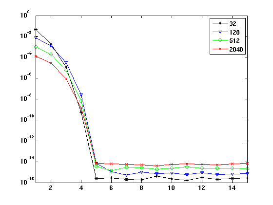
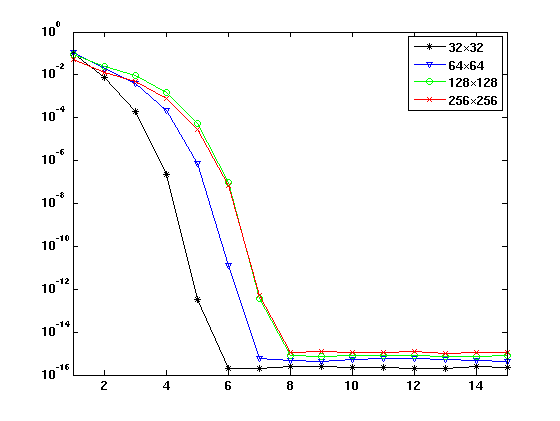
We report here some numerical tests supporting the results of the previous sections. For $N$ ranging from $32$ to $1024$, we integrate numerically (1) with the Barenblatt initial data for $m=4$ from $t=0$ to $t=20/32$ in one and two spatial dimensions, recording the number of Newton iterations, GMRES iterations and the error against the exact solution.

(a)	(b)

Figure 1: Crank-Nicholson scheme: Newton convergence history in one (a) and two (b) spatial dimensions

In figure 1 we plot the quantity $\|\mathbf{u}^{1,s}-\mathbf{u}^{1,s-1}\|$ during the Newton iterations $s=1,2,\ldots,30$ for computing the first time step. Different symbols and line colours correspond to different mesh sizes on the interval (1a) and on a square domain (1b). It is clear that the very good tolerance $10^{-6}$ is reached within a reasonable number of iterations: $4$ in one spatial dimension and $6$ in $\mathbb{R}^{2}$. This good convergence history is to a large extent not dependent on the chosen value for $m$ (see also [SDSC]).

Figure 2: Error of the numerical scheme in one and two dimensions, comparing with Implicit Euler

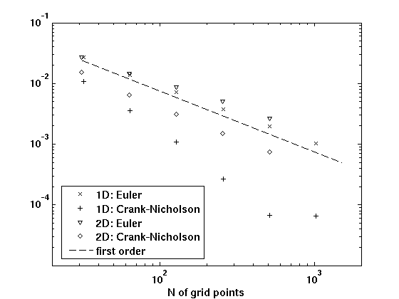
Using the Crank-Nicholson scheme, we observe a reduction of the error with respect to the first order Euler scheme (see Figure 2), even if the scheme does not converge with the expected order $2$. This is due to the presence of singularities in the exact solution. The least square fit of the errors obtained, in one dimension, with the Crank-Nicholson scheme and represented with plus signa in the figure gives that the error decays proportionally to $N^{-1.5}$. In two dimensions the rate of convergence is closer to $1$, but the errors are nevertheless lower than those obtained with the Implicit Euler scheme.

(a)	(b)

Figure 3: Crank-Nicholson scheme: GMRES iterations inside the Newton steps. (a): no preconditioning (the dashed line is the $N^{1/2}$ slope). (b): 1 V-cycle as preconditioner.

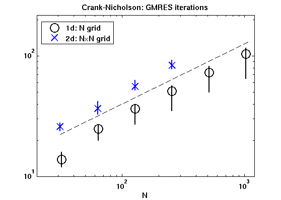
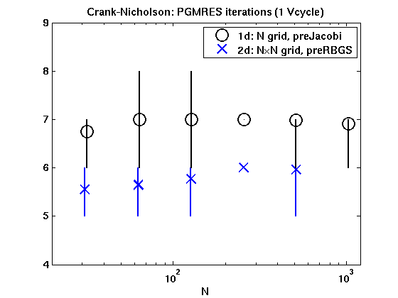
Finally, in Figure 3 we plot the number of iterations of the methods for linear system. For each value of $N$, we plot the average number of GMRES iterations performed by the algorithm (symbols), while the vertical lines span from the minimum to the maximum value recorded during the integration. Panel 3a compares the number of unpreconditioned GMRES iterations on different one- and two-dimensional grids with the $\sqrt{N}$ slope. Note that for the largest values of $N$, the two-dimensional experiments were not possible due to memory limitations on a PC with 8Gb of RAM. We employ MGM as preconditioner, choosing one damped Jacobi iteration as a presmoother in the V-cycle in the one-dimensional experiments, while for the two-dimensional we chose the more efficient Red-Black Gauss-Seidel. Panel 3b shows that applying one MGM V-cycle is optimal (constancy of iterations number for different $N$), robust (small variance in iterations number) and memory efficient (small number of iterations require small amount of storage memory in GMRES).

3 Marble sulfation

In this section we consider the model for the marble sulfation problem described in [ADDN04]. We describe the main features of the model only briefly, referring the reader to the original paper for the details and more comprehensive study of the properties of the solutions. [ADDN04] consider the (simplified) chemical reaction

$$\mathrm{CaCO_{3}}+\mathrm{SO_{2}}+\frac{1}{2}\mathrm{O_{2}}+2\mathrm{H_{2}O}\longrightarrow\mathrm{CaSO_{4}}\cdot 2\mathrm{H_{2}O}+\mathrm{CO_{2}}.$$

to account for the transformation of $\mathrm{CaCO_{3}}$ of the marble stone into gypsum $\mathrm{CaSO_{4}}\cdot 2\mathrm{H_{2}O}$, that is triggered in a moist atmosphere by the availability of $\mathrm{SO_{2}}$ at the marble surface and inside the pores of the stone. The two main variables of the model are $c(t,x)$ denoting the local concentration of calcium carbonate and $s(t,x)$ the local concentration of $\mathrm{SO_{2}}$. As the reaction proceeds, the calcium carbonate concentration is reduced from the initial value $c_{0}$, as $\mathrm{CaCO_{3}}$ is progressively replaced by gypsum. Denoting $\varphi_{0}$ and $\varphi_{g}$ the porosity of the pristine marble and of the gypsum, the model assumes that the porosity of the intermediate state is well approximated by linear interpolation

$$\varphi(c)=\varphi_{g}+(\varphi_{0}-\varphi_{g})\frac{c}{c_{0}}=\alpha c+\beta.$$

The constants $\alpha$ and $\beta$ depend on the porosity of the material involved. The model considered in [ADDN04] is described by the following system of PDEs:

$$\begin{cases}\displaystyle\frac{\partial\varphi(c)s}{\partial t}&=-\frac{a}{m_{c}}\varphi(c)sc+d\nabla\cdot\left(\varphi(c)\nabla s\right),\\[5.69054pt] \displaystyle\frac{\partial c}{\partial t}&=-\frac{a}{m_{s}}\varphi(c)sc.\end{cases}$$ (17)

The spatial domain $x\in\Omega$ in which (17) is set represents a piece of marble stone for which at least a portion of the boundary $\partial\Omega$ is in contact with the polluted atmosphere. In particular $\partial\Omega$ is in general split into two parts: one represents the outer surface of the marble sample, in contact with the air, and the complementary part that separates the portion of the marble object of the simulation and the rest of the monument.

(a)	(b)

Figure 4: Sample domains $\Omega$ for problem (17) are shown for the 1D setting (a) and 2D setting (b). The “brick pattern” area represents the marble stone, while the dotted area is air. The boundary is drawn with a solid line where Dirichlet boundary conditions are applied and with a dotted line where free-flow boundary conditions are imposed.

Examples of one and two-dimensional such domains are shown in Figure 4. In order to study the formation of a gypsum crust on a flat area of a monument, it is sufficient to take a 1-dimensional domain like in the left panel of the figure. In order to study a corner-like feature of a work of art, like the edge of a monument or a long decoration in relief, one would employ a 2-dimensional domain as the one in the right panel of the figure. Obviously more complex shapes need 3-dimensional domains representing faithfully the volume occupied by the marble.

Boundary conditions are set by imposing the value of $s$ on the outer boundary and by imposing free-flow conditions for $s$ on the inner boundary. In particular, as an example of a one-dimensional setting, we take $x\in\Omega=[0,1]$ where $x=0$ corresponds to the outer boundary of the marble stone, in contact with the polluted air, and $x=1$ the inner side. The boundary conditions are illustrated in Figure 4: they are of Dirichlet type, imposing $s(0,t)$ on the outer boundary and of free-flow type $\frac{\partial s}{\partial x}(1,t)=0$ on the inner side.

The parameters $m_{s}$ and $m_{c}$ are fixed by the physical properties of the species involved in the reaction and make sure that the mass balance is fulfilled. On the other hand $a$ represents the reaction rate and it depends (among other things) on the moisture of the air and on the temperature. [ADDN04] describes its central role in the analysis of the solutions of the model equations. In particular, if $u(t,x)$ is a solution of (17) for a given value of $a$, then $\tilde{u}(t,x)=u(t/a^{2},x/a)$ is a solution of (17) for $a=1$. This observation on one hand plays a fundamental role in establishing the long-time asymptotics of the solution and would allow to perform the simulations with $a=1$ and then rescale the numerical solutions appropriately to take the reaction rate into account. However, because of its role as fundamental physical parameter of the model, here we prefer to keep $a$ explicitly into the equations and perform simulations seeking numerical solution of the model in the form (17). Moreover this is beneficial in view of the more complete model including a non-constant $a$ has been described in [AFNT07].

We consider, as in [ADDN04] $\alpha=0.01$, $\beta=0.1$, $d=1$, $m_{s}=64.06$, $m_{c}=100.09$ and use $h=1/64$ or $h=1/128$ while varying $a$ from $1$ to $10^{5}$.

3.1 Discretization

As in the scalar case, we consider first and second order implicit time discretizations, namely the Implicit Euler scheme (Crandall-Liggett formula) and the Crank-Nicholson scheme. The general setup for the scheme is the same as in the scalar case: we discretize the spatial domain and the elliptic differential operator with finite differences, write the time-advancement problem as an implicit equation and set up a Newton scheme to solve it. This procedure is advantageous if the Newton scheme converges in a reasonable number of iterations and one can devise an optimal preconditioner for the linear system that has to be solved at each Newton step.

For the space discretization, we denote $x_{\xi}=0+\xi h\in\Omega$. Approximating the elliptic operator along the same lines as in (5), we consider the second order finite difference formula

$$\left.\partial_{x}(\varphi(c)\partial_{x}s)\right|_{x_{j}} = \frac{\varphi(c(x_{j+1/2}))(s(x_{j+1})-s(x_{j}))}{h^{2}}-$$ (19)

$$-\frac{\varphi(c(x_{j-1/2}))(s(x_{j})-s(x_{j-1}))}{h^{2}}.$$

This in turn suggests that we employ two staggered grids in the domain $\Omega$: the grid $x_{j}$ ($j\in\mathbb{N}$) with the unknowns $s^{n}_{j}$ for $s(t^{n},x_{j})$ and the grid $x_{j+1/2}$ ($j\in\mathbb{N}$) with the unknowns $c^{n}_{j+1/2}$ for $c(t^{n},x_{j+1/2})$. For short, we also denote $\varphi^{n}_{j+1/2}=\varphi(c^{n}_{j+1/2})$. For ease of reference, we will denote the two grid also by “integer grid” and “half-integer grid”.

We write explicitly the formulas for the Crank-Nicholson time discretization (3), pointing out that the case of Crandall-Liggett (Implicit Euler) scheme (2) can be similarly dealt with. Thus we consider the scheme that computes $s^{n}_{j}$ and $c^{n}_{j+1/2}$ solving the nonlinear system of equations:

$$\begin{cases}0=\mathbf{F}^{(s)}(\mathbf{s}^{n},\mathbf{c}^{n})=&\begin{aligned} &\Phi^{n}\mathbf{s}^{n}+\frac{\mathrm{\Delta}t}{2}\frac{a}{m_{c}}C^{n}\mathbf{s}^{n}+\frac{\mathrm{\Delta}t}{2}dL_{\varphi^{n}}\mathbf{s}^{n}\\ &-\Phi^{n-1}\mathbf{s}^{n-1}+\frac{\mathrm{\Delta}t}{2}\frac{a}{m_{c}}C^{n-1}\mathbf{s}^{n-1}+\frac{\mathrm{\Delta}t}{2}dL_{\varphi^{n-1}}\mathbf{s}^{n-1}\end{aligned}\\ 0=\mathbf{F}^{(c)}(\mathbf{s}^{n},\mathbf{c}^{n})=&\mathbf{c}^{n}-\mathbf{c}^{n-1}+\frac{\mathrm{\Delta}t}{2}\frac{a}{m_{s}}S^{n}\mathbf{c}^{n}+\frac{\mathrm{\Delta}t}{2}\frac{a}{m_{s}}S^{n-1}\mathbf{c}^{n-1}\end{cases}$$ (20)

where $\mathbf{s}^{n}=[s^{n}_{1},s^{n}_{2},\ldots]^{\mathsf{T}}$, $\mathbf{c}^{n}=[c^{n}_{1/2},c^{n}_{3/2},\ldots]^{\mathsf{T}}$ and

$$\Phi^{n}=\mathsf{diag}_{k}\left[\frac{\varphi^{n}_{k+1/2}+\varphi^{n}_{k-1/2}}{2}\right]$$ (21a)

$$C^{n}=\mathsf{diag}_{k}\left[\frac{\varphi^{n}_{k+1/2}c^{n}_{k+1/2}+\varphi^{n}_{k-1/2}c^{n}_{k-1/2}}{2}\right]$$ (21b)

$$L_{\varphi^{n}}=\mathsf{tridiag}_{k}\left[-\varphi^{n}_{k-1/2},\varphi^{n}_{k-1/2}+\varphi^{n}_{k+1/2},-\varphi^{n}_{k+1/2}\right]$$ (21c)

$$S=\mathsf{diag}_{k}\left[\varphi^{n}_{k+1/2}\left(\frac{s^{n}_{k+1}+s^{n}_{k}}{2}\right)\right]$$ (21d)

Note that equations (20) are not linear, since also the matrices $C$, $S$, $L_{\phi}$ and $\Phi$ depend on $\mathbf{c}^{n}$ and $\mathbf{s}^{n}$, either directly or via the (linear) function $\varphi$. It is important to note that the matrix $L_{\varphi}$ is defined as $L_{D}$ of (7), but it depends only on the half of the unknowns of the problem: precisely $L_{\varphi}$ depends on $\mathbf{c}$ and it multiplies $\mathbf{s}$ in formula (20).

The two staggered grids represent a sort of finite difference analogue of the approximation with $P1$ (for $s(x)$) and $P0$ (for $c(x)$) conforming finite elements considered in [ADDN04]. The results obtained here on preconditioning should also be applicable with little modifications in that case too.

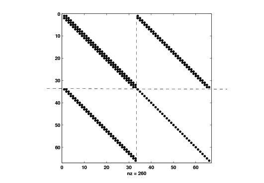
Boundary conditions are imposed considering $j=1,2,\ldots,N$ in (20) and assuming at all time steps a given value for $s_{0}$ (Dirichlet boundary condition at $x=0$) and that $s_{N+1}=s_{N-1}$ (homogeneous Neumann boundary condition at $x=1$). Thus the expressions of $\mathbf{F}^{(s)}_{1}$ and $\mathbf{F}^{(s)}_{N}$ are modified accordingly with respect to those in (20), together with the correspondent elements in the Jacobian (22). The $2N$ unknowns are collected in a vector $\mathbf{u}$ with the ordering $\mathbf{u}=[s_{1},s_{2},\ldots,s_{N},c_{1/2},\ldots,c_{N-1/2}]^{\mathsf{T}}$. The corresponding sparsity structure of the Jacobian matrix is illustrated in Figure 5. For the actual implementation it is easier to define the “porous concentration” and set the Dirichlet boundary condition as $\left.\varphi_{j-1/2}s_{j}\right|_{j=0}=\rho_{s_{0}}=1$.

Both the Crank-Nicholson and the Crandall-Liggett formulas give rise to an unconditionally stable scheme. Following the results previously established, in order to solve the nonlinear problem (20) we set up Newton iterations. To this end we need the Jacobian matrix, which is naturally split into four $N\times N$ block as

$$J=F^{\prime}=\left[\begin{array}[]{c|c}J^{s}_{s}&J^{s}_{c}\\ \hline\cr J^{c}_{s}&J^{c}_{c}\end{array}\right]\qquad\qquad\mathbf{u}=\begin{pmatrix}\mathbf{u}_{s}\\ \mathbf{u}_{c}\end{pmatrix}$$

The entries (disregarding boundary conditions) are:

$$\left[J^{s}_{s}\right]_{j,k}=\frac{\partial\mathbf{F}^{(s)}_{j}}{\partial s_{k}}= \frac{\varphi_{j+1/2}+\varphi_{j-1/2}}{2}\delta_{jk}+\frac{\mathrm{\Delta}t}{2}\frac{a}{m_{c}}\frac{\varphi_{j+1/2}c_{j+1/2}+\varphi_{j-1/2}c_{j-1/2}}{2}\delta_{jk}$$ (22)

$$+\frac{d}{2}\frac{\mathrm{\Delta}t}{h^{2}}\left[-\varphi_{j-1/2}\delta_{k,j-1}+(\varphi_{j-1/2}+\varphi_{j+1/2})\delta_{k,j}-\varphi_{j+1/2}\delta_{k,j+1}\right],$$

$$\left[J^{s}_{c}\right]_{j,k}=\frac{\partial\mathbf{F}^{(s)}_{j}}{\partial c_{k+1/2}}= \frac{\varphi^{\prime}_{j+1/2}s_{j}\delta_{jk}+\varphi^{\prime}_{j-1/2}s_{j}\delta_{j,k+1}}{2}$$

$$+\frac{\mathrm{\Delta}t}{2}\frac{a}{m_{c}}\frac{(\varphi^{\prime}_{j+1/2}c_{j+1/2}+\varphi_{j+1/2})\delta_{jk}+(\varphi^{\prime}_{j-1/2}c_{j-1/2}+\varphi_{j-1/2})\delta_{j,k+1}}{2}$$

$$+\frac{d}{2}\frac{\mathrm{\Delta}t}{h^{2}}\left[\varphi^{\prime}_{j-1/2}(s_{j}-s_{j-1})\delta_{j,k+1}-\varphi^{\prime}_{j+1/2}(s_{j+1}-s_{j})\delta_{j,k}\right],$$

$$\left[J^{c}_{s}\right]_{j,k}=\frac{\partial\mathbf{F}^{(c)}_{j+1/2}}{\partial s_{k}}= \frac{\mathrm{\Delta}t}{2}\frac{a}{m_{s}}\varphi_{j+1/2}c_{j+1/2}\frac{\delta_{j,k-1}+\delta_{jk}}{2},$$

$$\left[J^{c}_{c}\right]_{j,k}=\frac{\partial\mathbf{F}^{(c)}_{j+1/2}}{\partial c_{k+1/2}}= \left[1+\frac{\mathrm{\Delta}t}{2}\frac{a}{m_{s}}(\varphi^{\prime}_{j+1/2}c_{j+1/2}+\varphi_{j+1/2})\frac{s_{j+1}+s_{j}}{2}\right]\delta_{jk}.$$

Figure 5: Sparsity structure of the Jacobian matrix (22).

The sparsity structure of the Jacobian matrix with entries defined in (22) is shown in Figure 5. A more detailed analysis of the matrix will be carried out in the next section.

3.2 Solving the linear system

At each Newton iterations, we have to solve a linear system with matrix $J$, which is not symmetric and thus we employ GMRES as the main Krylov solver.

Figure 6: Number (average, min and max) of GMRES iterates per timestep with $A=1$, for 3 values of $N$. No preconditioner was used in this test. The dashed line indicates the $N^{1/2}$ slope.

We observe that the top-left $J^{s}_{s}$ block is given by

$$J^{s}_{s}=\Phi+\frac{\mathrm{\Delta}t}{2}\frac{a}{m_{c}}C+\frac{1}{2}\frac{\mathrm{\Delta}t}{h^{2}}dL_{\varphi}$$

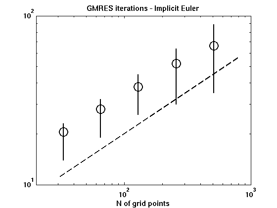
which is very similar to (9), except that the identity is replaced by the diagonal matrix $\Phi$ with $O(1)$ entries and the tridiagonal $Y$ term of (9) is not present, corresponding instead to the third term of the $J^{s}_{c}$ block. The extra term of $J^{s}_{s}$, involving the diagonal matrix $C$ has entries of order $\mathrm{\Delta}t$. Hence we expect $J_{s}^{s}$ to be spectrally not too different from $F^{\prime}$ of (9) and thus unpreconditioned GMRES iterations count to grow as $\sqrt{N}$, which is indeed confirmed in Figure 6, where we plot the average, minimum and maximum number of GMRES iterations needed in the case $a=1$ and for different values of the number of grid points $N$. A least square fit gives $N^{0.5217}$ for the number of iterations.

In order to devise a preconditioning strategy, given the structure of $J^{s}_{s}$, we can employ a V-cycle on this block, if we can deal optimally with the rest of the matrix. To this end we observe that the lower left block $J^{c}_{s}$ has nonzero entries only on two diagonals and these decay as $O(\mathrm{\Delta}t)$, while the bottom right block $J^{c}_{c}$ is the identity matrix plus a diagonal matrix with $O(\mathrm{\Delta}t)$ entries.

Theorem 3.1.

The upper triangular part of $J$,

$$P=\left[\begin{array}[]{c|c}J^{s}_{s}&J^{s}_{c}\\ \hline\cr{\bf 0}&J^{c}_{c}\end{array}\right]$$ (23)

is an optimal preconditioner for $J$, assuming that the function $\varphi(c)$ is bounded away from $0$, or equivalently that $\beta>0$.

Proof.

First observe that the diagonal blocks are nonsingular, so that

$$P^{-1}=\left[\begin{array}[]{c|c}(J^{s}_{s})^{-1}&-(J^{s}_{s})^{-1}(J^{s}_{c})(J^{c}_{c})^{-1}\\ \hline\cr{\bf 0}&(J^{c}_{c})^{-1}\end{array}\right]$$

and the preconditioned system has matrix

$$P^{-1}J=\left[\begin{array}[]{c|c}{\bf 1}-\left(J^{s}_{s}\right)^{-1}\left(J^{s}_{c}\right)\left(J^{c}_{c}\right)^{-1}\left(J^{c}_{s}\right)&{\bf 0}\\ \hline\cr\left(J^{c}_{c}\right)^{-1}\left(J^{c}_{s}\right)&{\bf 1}\end{array}\right]$$

where ${\bf 0}$ denotes the null matrix and ${\bf 1}$ the identity matrix.

We now show that all entries of $P^{-1}J$ are negligible except the diagonal ones. In fact $J^{c}_{c}$ is diagonal with entries equal to $1+O(\mathrm{\Delta}t)$ and thus its inverse has the same property. Since $J^{c}_{s}$ is tridiagonal with entries of $O(a\mathrm{\Delta}t)$, the same is true for the lower-left block of $P^{-1}J$. Gershgorin circles arising from the lower half of the matrix are thus centred at $1$ in the complex plane and have radii decaying as $O(\mathrm{\Delta}t)$.

We now turn to consider the upper half of the matrix, where we observe that $\|\left(J^{s}_{c}\right)\left(J^{c}_{c}\right)^{-1}\left(J^{c}_{s}\right)\|_{\infty}=O(\mathrm{\Delta}t)$ and thus it suffices to show that $\|\left(J^{s}_{s}\right)^{-1}\|_{\infty}$ is bounded to conclude that the Gershgorin circles arising from the upper half of the matrix are centred at $1+O(\mathrm{\Delta}t)$ in the complex plane and have radii decaying as $O(\mathrm{\Delta}t)$.

To this end, split

$$J^{s}_{s}=Z-W=Z({\bf 1}-Z^{-1}W)$$

where $Z$ is the diagonal part, which is

$$Z=\mathsf{diag}_{k}(z_{k}),\qquad z_{k}=\varphi_{k}+\mathrm{\Delta}t\frac{a}{m_{c}}\widetilde{\varphi}_{k}+2\frac{\mathrm{\Delta}t}{h^{2}}\varphi_{k}$$

where $\varphi_{k}=\tfrac{1}{2}(\varphi_{k+1/2}+\varphi_{k-1/2})$ and $\widetilde{\varphi}_{k}=\tfrac{1}{2}(\varphi_{k+1/2}c_{k+1/2}+\varphi_{k-1/2}c_{k-1/2})$. Since $Z$ is diagonal, we easily get the estimate

$$\|Z^{-1}\|_{\infty}\leq\max_{k}\frac{1}{z_{k}}=\frac{h^{2}}{\mathrm{\Delta}t}\max_{k}\frac{1}{2\varphi_{k}}\left(1+O\left(\tfrac{h^{2}}{\mathrm{\Delta}t}\right)\right)=O\left(\tfrac{h^{2}}{\mathrm{\Delta}t}\right)$$

Next observe that $Z^{-1}W=\tfrac{\mathrm{\Delta}t}{h^{2}}\mathsf{tridiag}_{k}(\tfrac{1}{z_{k}}[\varphi_{k-1/2},0,\varphi_{k+1/2}])$ and thus

$$\left\|Z^{-1}W\right\|_{\infty}=\left\|\mathsf{tridiag}_{k}\left(\frac{[\varphi_{k-1/2},0,\varphi_{k+1/2}]}{2\varphi_{k}+\tfrac{h^{2}}{\mathrm{\Delta}t}\varphi_{k}+h^{2}\tfrac{a}{m_{c}}\widetilde{\varphi}_{k}}\right)\right\|_{\infty}\leq\max_{k}\frac{2\varphi_{k}}{2\varphi_{k}+\tfrac{h^{2}}{\mathrm{\Delta}t}\varphi_{k}+h^{2}\tfrac{a}{m_{c}}\widetilde{\varphi}_{k}}\leq 1-Ch$$

for some small positive constant $C$. Therefore

$$\left\|\left({\bf 1}-Z^{-1}W\right)^{-1}\right\|_{\infty}\leq\sum_{j=0}^{\infty}\left\|Z^{-1}W\right\|_{\infty}^{j}\leq\frac{1}{Ch}$$

and

$$\|(J^{s}_{s})^{-1}\|_{\infty}=\left\|\left(Z\left({\bf 1}-Z^{-1}W\right)\right)^{-1}\right\|_{\infty}=\left\|\left({\bf 1}-Z^{-1}W\right)^{-1}\right\|_{\infty}\left\|Z^{-1}\right\|_{\infty}=O(1)$$

∎

Remark 3.2.

When applying the preconditioner, the block triangular system $P\mathbf{y}=\mathbf{b}$ is solved as

$$\mathbf{y}_{c}=(J^{c}_{c})^{-1}\mathbf{b}_{c}\qquad\mathbf{y}_{s}=(J^{s}_{s})^{-1}(\mathbf{b}_{s}-J^{s}_{c}\mathbf{y}_{c})$$

where the deponents $s$ and $c$ refer to the upper and, respectively, the lower half of the vectors. The previous result shows that the spectrum of $P^{-1}J$ is strongly clustered at $1$ independently on the discretization parameter $h$ and we expect the block-preconditioner $P$ to be optimal. For the whole preconditioner to be optimal, however we need an optimal solver for the $J^{s}_{s}$ block. However $J^{s}_{s}$ is the sum of two diagonal matrices and a tridiagonal matrix which is the discretization of a laplacian operator, regularised with the (strictly positive) function $\varphi(c(x))$, and thus has spectral properties close to those of $X_{N}$ studied in Section 2.3. As in the scalar case, a MGM (e.g. with 1 damped Jacobi as presmoother and a Galerkin approach with linear interpolation) is an optimal solver for this block.

(a)	(b)

Figure 7: Number (average, min and max) of GMRES iterates per timestep with $A=1$, for 3 values of $N$. (a) Block Gauss-Seidel and MGM for the upper left block was used as a preconditioner. Blue symbols and lines refer to the number of inner MGM iterations. (b) GMRES iterations when performing only 1 V-cycle of the MGM.

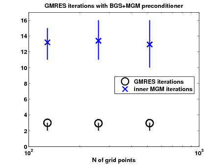
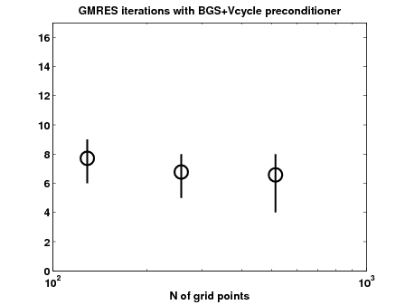
Our preconditioner is thus the Gauss-Seidel preconditioner at block level, with MGM on the $(s,s)$ block. The $(c,c)$ block does not need an inner preconditioner since it is diagonal and can be solved directly. This strategy yields an optimal preconditioner, i.e. renders the number of GMRES iterations independent from $N$, as confirmed by the numerical experiments shown in Figure 7). In the panel 7a we employ MGM driven to convergence as solver for the $(s,s)$ block in the preconditioner: GMRES converges in 2-3 iterations, requiring 10-15 MGM cycles at each iteration. In panel panel 7a we employ only a single MGM V-cycle as inner preconditioner for the $(s,s)$ block: the number of GMRES iterations grows slightly (6–8), but this procedure is overall more efficient. We observe an impressive series of good features: minimal average computational cost, minimal number of iterations, minimal variance in the latter number meaning a strong robustness of the procedure.

3.3 Simulations and performance of the algorithm

(a)	(b)

Figure 8: For different values of $a$, marble content and $\mathrm{SO}_{2}$ concentration inside the stone predicted by the model (17) for $t=1$.

(a)	(b)

Figure 9: Temporal evolution of the calcium carbonate and sulfate concentration predicted by the model (17) with $a=10^{4}$.

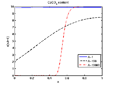
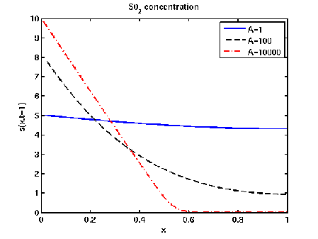
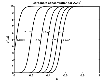
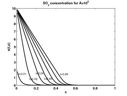
In Figure 8 we plot some typical curves obtained from the simulations with the model (17). Note that for bigger values $a$, the reaction is faster and a boundary layer appears. For $a=10^{4}$, Figure 9 shows the temporal evolution of the two main variables: while $\mathrm{SO_{2}}$ penetrates deeper and deeper into the stone (b), calcium carbonates is substituted by the more porous gypsum in a narrow spatial band where the curve $c(t,x)$ presents a boundary layer. Once formed, this transition region travels towards the interior of the stone (a). The self-similarity of the solutions of (17) under rescaling of the temporal and spatial variables mentioned at the beginning of Section 3 implies that the boundary layer observed for $a=10^{4}$ will also appear for lower values of $a$, if the solutions were sought for a larger temporal and spatial domain.

Newton iterations

In Figure 10 we plot the average, minimum and maximum number of Newton iterations used by the numerical method to solve the nonlinear equation (20) at each timestep.

Figure 10: Number (average, min and max) of Newton iterates per timestep.

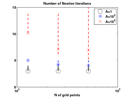
For $a=1$ (black circles) we note that the number of iterations is almost constant when the number of grid points is increased. Furthermore, for a given number of points employed in the discretization, the number of Newton iterations increases very moderately even when $a$ is increased by several orders of magnitude: e.g. for $N=128$ we need an average of $3$ Newton iterations per timestep for $a=1$, $5$ for $a=100$ (blue stars), and $10$ for $a=10000$ (red crosses). Finally we point out that for higher values of $N$, the number of Newton iterations decreases slightly since the grid becomes able to resolve better the boundary layer.

3.4 Asymptotics for the front position

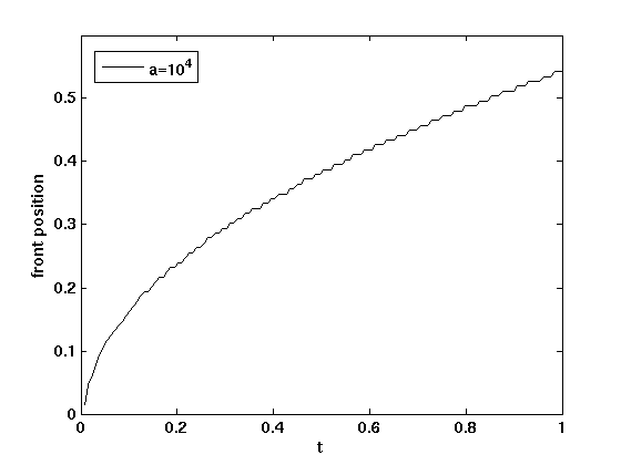
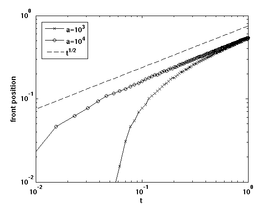
The asymptotic analysis of [GN07] predicts that the front of the travelling wave of $c(t,x)$ that separates the gypsum dominated phase from the carbonate dominated phase and that moves inwards in the marble sample asymptotically behaves as $x_{\text{front}}\sim\sqrt{t}$.

(a)	(b)

Figure 11: Gypsum-carbonate front position in a sulfation problem: numerical simulations (solid lines) and predicted asymptotics (dashed line) in b

We performed numerical experiments to test this prediction and to check how fast the front approaches this asymptotics. In order to perform the comparison, we extracted the information on the front position from the numerical solutions $c^{n}_{j+1/2}$ by identifying the gypsum-carbonate front with the point with steepest gradient of $c(t^{n},x)$.

For $a=10^{4}$, Figure 11a shows the position of the front. Note that the step-like behaviour of the numerical front that is apparent in some regions of the graph is due to the finite spatial resolution of the simulation ($h=1/128$). In order to check the asymptotics, we plot the position also in double logarithmic scale in Figure 11b, together with the $\sqrt{t}$ slope (dashed line). We note that both simulations agree with the slope of the asymptotics and that for the smaller value of $a$, the solution approaches the asymptotics more slowly.

3.5 Sample application in 2D

Figure 12: Number of GMRES iterations per Newton step: for each timestep we plot the average, minimum and maximum number of linear iterations. Without preconditioner: blue, crosses. With V-cycle preconditioner: black, circles.

In this section we present a numerical simulation of equations (17) in the two dimensional setting of figure 4. We consider again two staggered quadrangular regular grids in $\Omega=[0,1]\times[0,1]$. When using $N$ points per direction, we denote $x_{\xi}=\xi/N$ and $y_{\xi}=\xi/N$. We generalize the construction of Section 3.1 considering two staggered grids: the integer grid is the set of points $\{(x_{i},y_{j})\}_{i,j=0}^{N}$ carrying the values $s_{i,j}$ of the $\mathrm{SO_{2}}$ concentration field $s(x,y)$ and the half-integer grid is the set $\{(x_{i+1/2},y_{j+1/2})\}_{i,j=1}^{N}$ carrying the values $c_{i+1/2,j+1/2}$ of the calcium carbonate concentration field. The discretization of the elliptic operator is then generalized in the usual way to the two dimensional setting, and the new form of the fixed point problem (20) and its laplacian (22) are derived. The numerical scheme now requires, at each timestep, the solution of a system of $2N^{2}$ nonlinear equations. Using again the Newton method, at each iteration we need to solve a sparse linear system with a matrix of dimension $2N^{2}\times 2N^{2}$.

The Jacobian matrix has the same block structure described in the one-dimensional case (see also Figure 5). Since it is not symmetric, we use GMRES as main Krylov solver with specialised structured preconditioners as in the one dimensional case. The main difference in fact is that now the $J^{s}_{s}$ block is a weighted two-dimensional laplacian plus diagonal corrections that are small (in the sense of order of $h$). The $J^{c}_{c}$ block remains diagonal with elements equal to $1+O(\mathrm{\Delta}t)$ and the preconditioner (23) can be applied. The off-diagonal blocks have more non-zero diagonals, but their elements are still small and Theorem 3.1 can be generalized to the two-dimensional setting.

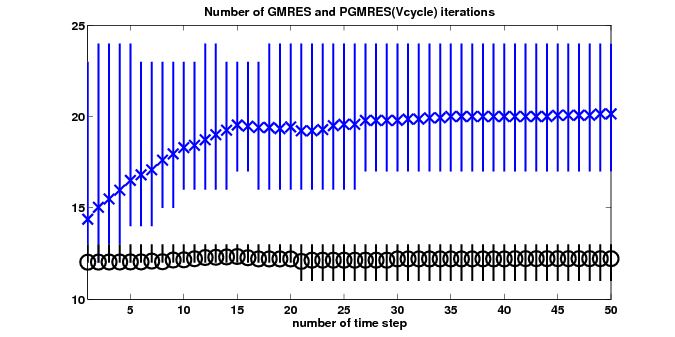
Here we consider only the best preconditioner of those evaluated in the one dimensional setting, namely the upper triangular part of the Jacobian matrix, where we perform only 1 V-cycle on the $(s,s)$ block. In Figure 12 we study the effectiveness of this preconditioning technique. On a $32\times 32$ grid, we observe that unpreconditioned GMRES requires an average of $15$ to $20$ iterations to solve the Jacobian linear system in each Newton step, with frequent peaks of $24$ iterations (blue crosses in the figure are the average values, blue lines the minimum to maximum range). Moreover the number of iterations is not constant but depends on the timestep. On the contrary the preconditioned method employs always an average of $12$ PGMRES iterations, with little variability both within the time step and across the different times (black circles and lines).

Figure 13: Simulation of marble sulfation in two dimensions.

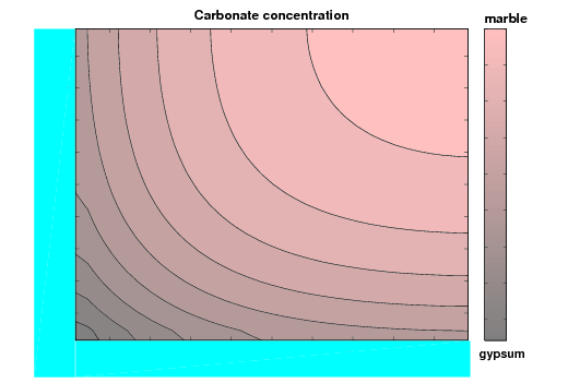
In Figure 13 we plot the solution obtained for $a=10$. We recall the the marble is in contact with the polluted air at the bottom and left boundary (cyan regions), while at the top and right boundary we apply free flow conditions. Both the colour code and the isolines refer to the carbonate concentration in the stone. We observe a clear deformation of the $\mathrm{CaCO_{3}}$ field near the corner, clearly indicating that $\mathrm{SO_{2}}$, penetrating from both sides, causes an enhanced loss of material: if the gypsum crust were to fall off here, the sharp edge would be chipped off and the shape of the stone would be permanently changed. This simulation, although performed at low resolution ($32\times 32$ grids) and with a moderate value of $a$, already indicates the relevance of our project of developing accurate numerical simulators for realistic geometries of the domain $\Omega$ in two and three dimensions.

4 Conclusions and future developments

The novel contribution of this paper relied in the proposal of a fully implicit numerical method for dealing with the nonlinear PDE, in its convergence and stability analysis, and in the study of the related computational cost. Indeed the nonlinear nature of the underlying mathematical model required the application of a fixed point scheme. We have identified the classical Newton method in which, at every step, the solution of a large, locally structured, linear system has been handled by using specialised iterative or multi-iterative solvers. In particular, the spectral analysis of the relevant matrices has been crucial for identifying appropriate preconditioned Krylov methods with efficient V-cycle preconditioners. Numerical experiments for the validation of our analysis complement this contribution, which is aimed to provide a non-invasive tool for a quantitative forecast of the damage evolution in a given monument.

In particular we considered the application of the above-mentioned techniques to the numerical approximation of a mathematical model describing the damage of marble monuments by the sulfation process. The use of our resulting fast integration algorithms allows to exploit the model and its predictive power for the strategy known as planned conservation, that is the novel approach that privileges the study and prevention of the damages to delay and optimise the actual restoration works. We showed both one dimensional and two dimensional numerical simulations, using simple domains.

For future work, two main directions appear naturally. The first is to finite element methods for the space discretization in order to deal with more realistic domains in 2D and 3D, that can model a real architectural item with a complicate geometry. In this setting we expect algebraic (linear) MGM or even nonlinear multigrid (FAS) to play an important role. The other natural extension of the numerical treatment for the sulfation problem involves considering the 3-equations model in [AFNT07] and/or a model for a remediation technique, like the one in [CGN⁺09] (this will include consolidation models that is systems of the type $u_{t}=(D(u)(p(u)_{x}))_{x}$). As a long term goal, being able to simulate both the damage and the remediation process with validated mathematical models and numerical methods would allow to perform numerical experiments of restoration works.

References

- [ADDN04] D. Aregba Driollet, F. Diele, and R. Natalini. A mathematical model for the aggression to calcium carbonate stones: numerical approximation and asymptotic analysis. SIAM J. Appl. Math., 64(5):1636–1667, 2004.
- [AFNT07] G. Alì, V. Furuholt, R. Natalini, and I. Torcicollo. A mathematical model of sulphite chemical aggression of limestones with high permeability. I. Modeling and qualitative analysis. Transp. Porous Media, 69(1):109–122, 2007.
- [BBR79] A.E. Berger, H. Brezis, and J.C.W Rogers. A numerical method for solving the problem . RAIRO numerical analysis, 13:297–312, 1979.
- [BLTR00] R. Bugini, M. Laurenzi Tabasso, and M. Realini. Rate of formation of black crusts on marble. A case study. J. Cultural Heritage, pages 111–116, 2000.
- [BP72] H. Brézis and A. Pazy. Convergence and approximation of semigroups of nonlinear operators in Banach spaces. J. Functional Analysis, 9:63–74, 1972.
- [CGN+09] F. Clarelli, C. Giavarini, R. Natalini, C. Nitsch, and M.L Santarelli. Mathematical models for the consolidation processes in stones. In Proc. of “International Symposium: Stone Consolidation in Cultural Heritage - research and practice”. Lisbona, May 2008., 2009. to appear.
- [CL71] M.G. Crandall and T.M. Liggett. Generation of Semi-Groups of non linear transformations on general Banach spaces. Amer. J. Math., 93:265–298, 1971.
- [CNPS07] F. Cavalli, G. Naldi, G. Puppo, and M. Semplice. High-order relaxation schemes for non linear degenerate diffusion problems. SIAM Journal on Numerical Analysis, 45(5):2098–2119, 2007.
- [GKPC89] K.L. Gauri, N.P. Kulshreshtha, A.R. Punuru, and A.N. Chowdhury. Rate of decay of marble in laboratory and outdoor exposure. J. Mater. Civil Eng., pages 73–85, 1989.
- [GN05] F. R. Guarguaglini and R. Natalini. Global existence of solutions to a nonlinear model of sulphation phenomena in calcium carbonate stones. Nonlinear Anal. Real World Appl., 6(3):477–494, 2005.
- [GN07] F. R. Guarguaglini and R. Natalini. Fast reaction limit and large time behavior of solutions to a nonlinear model of sulphation phenomena. Comm. Partial Differential Equations, 32(1-3):163–189, 2007.
- [Gre97] Anne Greenbaum. Iterative methods for solving linear systems, volume 17 of Frontiers in Applied Mathematics. Society for Industrial and Applied Mathematics (SIAM), Philadelphia, PA, 1997.
- [GSNF08] C. Giavarini, M.L. Santarelli, R. Natalini, and F. Freddi. A nonlinear model of sulphation of porous stones: numerical simulations and preliminary laboratory assessments. J. Cultural Heritage, 9:14–22, 2008.
- [Hac85] Wolfgang Hackbusch. Multigrid methods and applications, volume 4 of Springer Series in Computational Mathematics. Springer-Verlag, Berlin, 1985.
- [Hay82] F.H. Hayne. Deterioration of marble. Durability Build. Mater., (1):241–254, 1982.
- [Lip89] W.T. Lipfert. Atmospheric damage to calcareous stones: comparison and reconciliation of recent experimental findings. Atmos. Environ., 23:415–429, 1989.
- [MNV87] E. Magenes, R. H. Nochetto, and C. Verdi. Energy error estimates for a linear scheme to approximate nonlinear parabolic problems. RAIRO Modél. Math. Anal. Numér., 21(4):655–678, 1987.
- [OR70] J. M. Ortega and W. C. Rheinboldt. Iterative solution of nonlinear equations in several variables. Academic Press, New York, 1970.
- [Saa03] Yousef Saad. Iterative methods for sparse linear systems. Society for Industrial and Applied Mathematics, Philadelphia, PA, second edition, 2003.
- [SC93] S. Serra-Capizzano. Multi-iterative methods. Comput. Math. Appl., 26(4):65–87, 1993.
- [SC06] Stefano Serra-Capizzano. The GLT class as a generalized Fourier analysis and applications. Linear Algebra Appl., 419(1):180–233, 2006.
- [SDSC] M. Semplice, M. Donatelli, and S. Serra-Capizzano. Multigrid and preconditioning strategies for implicit PDE solvers for degenerate parabolic equations. IMA. Submitted. Preprint arXiv:0907.2600v2.
- [SDSC09] M. Semplice, M. Donatelli, and S. Serra-Capizzano. Preconditioned fully implicit pde solvers for degenerate parabolic equations with applications to monument conservation. http:www.arXiv.org, (0907.2600v1), 15 July 2009.
- [Til98] P. Tilli. Locally Toeplitz sequences: spectral properties and applications. Linear Algebra Appl., 278(1-3):91–120, 1998.
- [TOS01] U. Trottenberg, C. W. Oosterlee, and A. Schüller. Multigrid. Academic Press Inc., San Diego, CA, 2001. With contributions by A. Brandt, P. Oswald and K. Stüben.
- [V0́7] J. L. Vázquez. The porous medium equation. Oxford Mathematical Monographs. The Clarendon Press Oxford University Press, Oxford, 2007. Mathematical theory.