Induced fermionic current in toroidally compactified spacetimes with applications to cylindrical and toroidal nanotubes

Abstract

The vacuum expectation value of fermionic current is evaluated for a massive spinor field in spacetimes with arbitrary number of toroidally compactified spatial dimensions in the presence of a constant gauge field. By using the Abel-Plana type summation formula and the zeta function technique we present the fermionic current in two different forms. Non-trivial topology of the background spacetime leads to the Aharonov-Bohm effect for the fermionic current induced by the gauge field. The current is a periodic function of the magnetic flux with the period equal to the flux quantum. In the absence of gauge field it vanishes for special cases of untwisted and twisted fields. Applications of general formulae to Kaluza-Klein type models and to cylindrical and toroidal carbon nanotubes are given. In the absence of magnetic flux the total fermionic current in carbon nanotubes vanishes, due to the cancellation of contributions from two different sublattices of the hexagonal lattice of graphene.

PACS numbers: 03.70.+k, 11.10.Kk, 61.46.Fg

1 Introduction

In many physical problems we need to consider some model on a background of manifold having compact spatial dimensions along which dynamical variables satisfy some prescribed periodicity conditions. Incomplete list of applications where the topological effects play an important role includes Kaluza-Klein type models, supergravity and superstring theories. From an inflationary point of view, universes with compact dimensions, under certain conditions, should be considered as a general rule rather than an exception [1]. Models of a compact universe with non-trivial topology may play an important role by providing proper initial conditions for inflation. An interesting application of the field theoretical models with non-trivial topology of spatial dimensions appeared in nanophysics recently [2]. The long-wavelength description of the electronic states in graphene can be formulated in terms of Dirac-like theory in 3-dimensional spacetime with the Fermi velocity playing the role of a speed of light (see, e.g., Refs. [3, 4]). Single-walled carbon nanotubes are generated by rolling up a graphene sheet to form a cylinder and the background spacetime for the corresponding Dirac-like theory has a topology $R^{2}\times S^{1}$. The compactification in the direction along the cylinder axis gives another class of graphene structures called toroidal carbon nanotubes with the background topology $R^{1}\times(S^{1})^{2}$ [5].

The compactification of spatial dimensions leads to a number of interesting field theoretical effects which include instabilities in interacting field theories, topological mass generation and symmetry breaking. In quantum field theory the boundary conditions imposed on fields along compact dimensions change the spectrum of vacuum fluctuations. The resulting energies and stresses are known as the topological Casimir effect. (For the topological Casimir effect and its role in cosmology see [6]-[10] and references therein.) Note that Casimir forces between material boundaries are presently attracting much experimental attention [11]. In the Kaluza-Klein type models this effect has been used as a stabilization mechanism for moduli fields which parametrize the size and the shape of the extra dimensions. The Casimir energy can also serve as a model of dark energy needed for the explanation of the present accelerated expansion of the universe (see [12] and references therein).

The effects of the toroidal compactification of spatial dimensions on the properties of quantum vacuum for various spin fields have been discussed by several authors (see, for instance, [6]-[13] and references therein). One-loop quantum effects for the scalar and fermionic fields in de Sitter spacetime with toroidally compactified dimensions are studied in Refs. [14, 15]. In previous papers [16, 17] we have investigated the fermionic condensate and the vacuum expectation value of the energy-momentum tensor for a massive spinor field in higher-dimensional spacetimes with toroidally compactified spatial dimensions. These expectation values are among the most important quantities that characterize the properties of the quantum vacuum. Another important characteristic is the vacuum expectation value of fermionic current. Although the corresponding operator is local, due to the global nature of the vacuum, this quantity carries an important information about the global properties of the background spacetime. In addition to describing physical structure of the quantum field at a given point, the current acts as the source in the Maxwell equations. It therefore plays an important role in modelling a self-consistent dynamics involving the electromagnetic field.

In the present paper, we investigate one-loop quantum effects on the fermionic current arising from vacuum fluctuations of a massive fermionic field on the background of spacetimes with an arbitrary number of toroidally compactified spatial dimensions. We will assume generalized periodicity conditions along the compactified dimensions with arbitrary phases and the presence of a constant gauge field. A non-zero gauge field defined on topologically non-trivial background leads to the Aharonov-Bohm effect for the vacuum expectation value of fermionic current. Note that fermionic current in spacetime with non-trivial topology induced by a cosmic string has been investigated in Refs. [18].

This paper is organized as follows. In the next section, we consider vacuum expectation value of the fermionic current in the background spacetime with spatial topology $R^{p}\times(S^{1})^{q}$ in the presence of a constant gauge field. The corresponding expression is derived by using the Abel-Plana type summation formula. An equivalent representation is obtained in Section 3 within the framework of the generalized zeta function approach. In Section 4 we apply the general formula for the evaluation of the fermionic current in cylindrical and toroidal nanotubes within the framework of Dirac-like model for electrons in graphene. Main results are summarized in Section 5.

2 Vacuum expectation value of the fermionic current

We consider the quantum fermionic field $\psi$ on a background of $(D+1)$-dimensional flat spacetime with spatial topology $R^{p}\times(S^{1})^{q}$, $p+q=D$. The Cartesian coordinates along uncompactified and compactified dimensions are denoted as $\mathbf{z}_{p}=(z^{1},\ldots,z^{p})$ and $\mathbf{z}_{q}=(z^{p+1},\ldots,z^{D})$, respectively. The length of the $l$-th compact dimension we denote as $L_{l}$. Hence, for coordinates one has $-\infty<z^{l}<\infty$ for $l=1,\ldots,p$, and $0\leqslant z^{l}\leqslant L_{l}$ for $l=p+1,\ldots,D$. We assume that along the compact dimensions the field obeys the generic quasiperiodic boundary conditions,

$$\psi(t,\mathbf{z}_{p},\mathbf{z}_{q}+L_{l}\mathbf{e}_{l})=e^{2\pi i\alpha_{l}}\psi(t,\mathbf{z}_{p},\mathbf{z}_{q}),$$ (1)

with constant phases $\alpha_{l}$ and with $\mathbf{e}_{l}$ being the unit vector along the direction of the coordinate $z^{l}$, $l=p+1,\ldots,D$. Condition (1) includes the periodicity conditions for both untwisted and twisted fermionic fields as special cases with $\alpha_{l}=0$ and $\alpha_{l}=1/2$, respectively. As is discussed below, the special cases $\alpha_{l}=0,\pm 1/3$ are realized in nanotubes.

Dynamics of the massive spinor field is governed by the Dirac equation

$$i\gamma^{\mu}D_{\mu}\psi-m\psi=0\ ,\;D_{\mu}=\partial_{\mu}+ieA_{\mu},$$ (2)

where $A_{\mu}$ is the vector potential for the external electromagnetic field. In the discussion below we assume that $A_{\mu}=\mathrm{const}$. Though the corresponding magnetic field strength vanishes, the non-trivial topology of the background spacetime leads to Aharonov-Bohm-like effects for physical observables. In particular, as it is shown below, the expectation value of fermionic current depends on $A_{\mu}$. In the $(D+1)$-dimensional spacetime, the Dirac matrices are $N\times N$ matrices with $N=2^{[(D+1)/2]}$, where the square brackets mean the integer part of the enclosed expression. We assume that these matrices are given in the Dirac representation:

$$\gamma^{0}=\left(\begin{array}[]{cc}1&0\\ 0&-1\end{array}\right),\;\gamma^{\mu}=\left(\begin{array}[]{cc}0&\sigma_{\mu}\\ -\sigma_{\mu}^{+}&0\end{array}\right),\;\mu=1,2,\ldots,D.$$ (3)

From the anticommutation relations for the Dirac matrices one has $\sigma_{\mu}\sigma_{\nu}^{+}+\sigma_{\nu}\sigma_{\mu}^{+}=2\delta_{\mu\nu}$. In the case $D=2$ we have $N=2$ and the Dirac matrices are taken in the form $\gamma^{\mu}=(\sigma_{\text{P}3},i\sigma_{\text{P}1},i\sigma_{\text{P}2})$, with $\sigma_{\text{P}\mu}$ being the $2\times 2$ Pauli matrices. We are interested in the effects of non-trivial topology on the vacuum expectation value (VEV) of fermionic current $j^{\mu}=\bar{\psi}\gamma^{\mu}\psi$, where $\bar{\psi}$ is the Dirac conjugated spinor. Note that the fermionic condensate and the VEV of the energy-momentum tensor in the model under consideration were evaluated in Ref. [16] in the absence of gauge field.

By expanding the field operator in terms of annihilation and creation operators, the VEV of fermionic current is presented as the sum over all modes

$$\langle 0|j^{\mu}|0\rangle=\sum_{\beta}\bar{\psi}_{\beta}^{(-)}(x)\gamma^{\mu}\psi_{\beta}^{(-)}(x),$$ (4)

where $\{\psi_{\beta}^{(+)},\psi_{\beta}^{(-)}\}$ is the complete set of positive- and negative-frequency eigenfunctions satisfying the periodicity conditions (1) along compact dimensions. Here, $\beta$ is a set of quantum numbers specifying the solutions. The dependence of the eigenfunctions on the spacetime coordinates can be taken in the form $e^{i\mathbf{k}\cdot\mathbf{r}-i\omega t}$, with the wave vector $\mathbf{k}$. From the Dirac equation for the positive- and negative-frequency solutions we find

$$\psi_{\beta}^{(+)} = A_{\beta}^{(+)}e^{i\mathbf{k}\cdot\mathbf{r}-i\omega t}\left(\begin{array}[]{c}w_{\sigma}^{(+)}\\ \frac{\omega-eA_{0}-m}{(\mathbf{k}-e\mathbf{A})^{2}}(\mathbf{k}-e\mathbf{A})\cdot\boldsymbol{\sigma}^{+}w_{\sigma}^{(+)}\end{array}\right),$$ (7)

$$\psi_{\beta}^{(-)} = A_{\beta}^{(-)}e^{-i\mathbf{k}\cdot\mathbf{r}+i\omega t}\left(\begin{array}[]{c}\frac{\omega+eA_{0}-m}{(\mathbf{k}+e\mathbf{A})^{2}}(\mathbf{k}+e\mathbf{A})\cdot\boldsymbol{\sigma}w_{\sigma}^{(-)}\\ w_{\sigma}^{(-)}\end{array}\right),$$ (10)

where $\beta=(\mathbf{k},\sigma)$, $A_{\mu}=(A_{0},-\mathbf{A})$, and $\boldsymbol{\sigma}=(\sigma_{1},\sigma_{2},\ldots,\sigma_{D})$. In these expressions $w_{\sigma}^{(+)}$, $\sigma=1,\ldots,N/2$, are one-column matrices having $N/2$ rows with the elements $w_{\sigma l}^{(+)}=\delta_{\sigma l}$, and $w_{\sigma}^{(-)}=iw_{\sigma}^{(+)}$. The frequency and the wave vector are connected by the relation $\left(\omega\mp eA_{0}\right)^{2}=(\mathbf{k}\mp e\mathbf{A})^{2}+m^{2}$ for the function $\psi_{\beta}^{(\pm)}$.

The coefficients $A_{\beta}^{(\pm)}$ are found from the orthonormalization condition $\int d^{3}x\,\psi_{\beta}^{(\pm)+}\psi_{\beta^{\prime}}^{(\pm)}=\delta_{\beta\beta^{\prime}}$, where $\delta_{\beta\beta^{\prime}}$ is understood as the Dirac delta function for continuous indices and the Kronecker delta for discrete ones. From this condition one finds

$$A_{\beta}^{(\pm)2}=\frac{1}{(2\pi)^{p}V_{q}}\left[1+\frac{\left(\omega\mp eA_{0}-m\right)^{2}}{(\mathbf{k}\mp e\mathbf{A})^{2}}\right]^{-1},$$ (11)

where $V_{q}=L_{p+1}\cdots L_{D}$ is the volume of the compact subspace.

We decompose the wave vector into components along the uncompactified and compactified dimensions: $\mathbf{k}=(\mathbf{k}_{p},\mathbf{k}_{q})$, $k=\sqrt{\mathbf{k}_{p}^{2}+\mathbf{k}_{q}^{2}}$. The eigenvalues for the components along the compact dimensions are determined from boundary conditions (1):

$$k_{l}=2\pi(n_{l}+\alpha_{l})/L_{l},\;n_{l}=0,\pm 1,\pm 2,\ldots,\;l=p+1,\ldots,D.$$ (12)

For the components along the uncompactified dimensions one has $-\infty<k_{l}<\infty$, $l=1,\ldots,p$.

Substituting the eigenfunctions (10) into the mode sum formula (4) and by using the properties of Dirac matrices one finds

$$\langle 0|j^{0}|0\rangle = \frac{N}{2V_{q}}\int\frac{d\mathbf{k}_{p}}{(2\pi)^{p}}\sum_{\mathbf{n}_{q}\in\mathbf{Z}^{q}}1,$$ (13)

$$\langle 0|j^{l}|0\rangle = \frac{N}{2V_{q}}\int\frac{d\mathbf{k}_{p}}{(2\pi)^{p}}\sum_{\mathbf{n}_{q}\in\mathbf{Z}^{q}}\frac{(\mathbf{k}+e\mathbf{A})_{l}}{\sqrt{(\mathbf{k}+e\mathbf{A})^{2}+m^{2}}},$$ (14)

with $l=1,2,\ldots,D$ and $\mathbf{n}_{q}=(n_{p+1},\ldots,n_{D})$. In order to give a meaning to divergent expressions, it is necessary to regularize them. Here we use a Pauli-Villars gauge-invariant regularization. An alternative way is to introduce a cutoff function. Introducing regulator fields with large masses $M_{s}$, $s=1,2,\ldots,S$, for the regularized expressions one finds

$$\langle 0|j^{0}|0\rangle_{\text{reg}} = \frac{N}{2V_{q}}\int\frac{d\mathbf{k}_{p}}{(2\pi)^{p}}\sum_{\mathbf{n}_{q}\in\mathbf{Z}^{q}}\sum_{s=0}^{S}C_{s},$$ (15)

$$\langle 0|j^{l}|0\rangle_{\text{reg}} = \frac{N}{2V_{q}}\int\frac{d\mathbf{k}_{p}}{(2\pi)^{p}}\sum_{\mathbf{n}_{q}\in\mathbf{Z}^{q}}\sum_{s=0}^{S}\frac{C_{s}(\mathbf{k}+e\mathbf{A})_{l}}{\sqrt{(\mathbf{k}+e\mathbf{A})^{2}+M_{s}^{2}}},$$ (16)

with $C_{0}=1$ and $M_{0}=m$. Under the conditions $\sum_{s=0}^{S}C_{s}M_{s}^{2n}=0$,$\;n=0,1,\ldots,[D/2]$, these expressions are finite. After the renormalization subtractions the regulator is removed taking the limit $M_{s}\rightarrow\infty$, $s\geqslant 1$. From formula (15) it follows that the VEV of the temporal component of the fermionic current is renormalized to zero. Shifting the integration variable in (16), we directly see that $\langle 0|j^{l}|0\rangle_{\text{reg}}=0$ for the components with $l=1,\ldots,p$. Hence, the renormalized VEV of the fermionic current is different from zero only for the components along the compact dimensions.

Shifting the integration variables, $k_{l}+eA_{l}\rightarrow k_{l}$, $l=1,\ldots,p$, for these components one finds

$$\langle 0|j^{r}|0\rangle_{\text{reg}}=\frac{N}{2V_{q}}\int\frac{d\mathbf{k}_{p}}{(2\pi)^{p}}\sum_{\mathbf{n}_{q}\in\mathbf{Z}^{q}}\sum_{s=0}^{S}\frac{2\pi C_{s}(n_{r}+\tilde{\alpha}_{r})/L_{r}}{\sqrt{\mathbf{k}_{p}^{2}+\sum_{l=p+1}^{D}[2\pi(n_{l}+\tilde{\alpha}_{l})/L_{l}]^{2}+M_{s}^{2}}},$$ (17)

with $r=p+1,\ldots,D$, and we have introduced the notation

$$\tilde{\alpha}_{l}=\alpha_{l}+eA_{l}L_{l}/(2\pi).$$ (18)

Hence, the VEV of the fermionic current depends on components of the vector potential along the compact dimensions alone. We present the second term on the right of (18) as $eA_{l}L_{l}/(2\pi)=N_{l}+\gamma_{l}$, where $N_{l}$ is an integer number and $\gamma_{l}$ is the fractional part. As it is seen from formula (17), only the fractional part leads to nontrivial effects. Another point to be mentioned is that the presence of a gauge field leads to the shift of the phases in the quasiperiodic boundary conditions along compact dimensions. This feature is applicable to the fermionic condensate and the VEV of the energy-momentum tensor as well. In particular, the formulae for these quantities in the presence of a constant gauge field are obtained from the corresponding formulae in Ref. [16] by the replacement $\alpha_{l}\rightarrow\tilde{\alpha}_{l}$.

The property that the VEVs depend on the phases $\alpha_{l}$ and on the vector potential components along compact dimensions in the combination (18) can also be seen by the gauge transformation $A_{\mu}=A_{\mu}^{\prime}+\partial_{\mu}\Lambda(x)$, $\psi(x)=\psi^{\prime}(x)e^{-ie\Lambda(x)}$, with the function $\Lambda(x)=A_{\mu}x^{\mu}$. The new function $\psi^{\prime}(x)$ satisfies Dirac equation with $A_{\mu}^{\prime}=0$ and the quasiperiodicity conditions similar to (1) with the replacement $\alpha_{l}\rightarrow\tilde{\alpha}_{l}$. Corresponding eigenspinors are given by expressions (7), (10) with $\mathbf{A}=0$ and the eigenvalues for the wave vector components along compact dimensions are defined by $k_{l}=2\pi(n_{l}+\tilde{\alpha}_{l})/L_{l}$. In the new gauge, the regularized VEVs are given by Eqs. (15) and (16) with $\mathbf{A}=0$. The latter coincide with (15) and (16) after the shift $k_{l}+eA_{l}\rightarrow k_{l}$, $l=1,\ldots,p$, of the integration variables for the components along uncompactified dimensions.

We will evaluate the VEV of fermionic current by two equivalent methods: by applying the Abel-Plana type summation formula and using the zeta-function technique. In the first approach we apply to the series over $n_{r}$ in Eq. (17) the following summation formula:

$$\sum_{n_{r}=-\infty}^{\infty}g(n_{r}+\tilde{\alpha}_{r})f(|n_{r}+\tilde{\alpha}_{r}|)=\int_{0}^{\infty}du\,\left[g(u)+g(-u)\right]f(u)$$

$$\quad+i\int_{0}^{\infty}du\left[f(iu)-f(-iu)\right]\sum_{\lambda=\pm 1}\frac{g(i\lambda u)}{e^{2\pi(u+i\lambda\tilde{\alpha}_{r})}-1}.$$ (19)

This formula is obtained by combining the summation formulae given in Ref. [19] (see also [16]). In the special case of $g(x)=1$, $\tilde{\alpha}_{r}=0$ formula (19) reduces to the standard Abel-Plana formula (for the applications of the Abel-Plana formula and its generalizations in quantum field theory see [6, 20, 21]). Taking in Eq. (19)

$$g(x)=2\pi x/L_{r},\;f(x)=\left[\mathbf{k}_{p}^{2}+\omega_{\mathbf{n}_{q-1}^{r}}^{2}+(2\pi x/L_{r})^{2}\right]^{-1/2},\;$$ (20)

with

$$\omega_{\mathbf{n}_{q-1}^{r}}^{2}=\sum_{l=p+1,l\neq r}^{D}[2\pi(n_{l}+\tilde{\alpha}_{l})/L_{l}]^{2}+m^{2},$$ (21)

and $\mathbf{n}_{q-1}^{r}=(n_{p+1},\ldots,n_{r-1},n_{r+1},\ldots,n_{D})$, we see that the first integral on the right-hand side of this formula vanishes. The contribution of the second integral to the regularized VEV is finite in the limit $M_{s}\rightarrow\infty$, $s\geqslant 1$, and in this term the regulator can be safely removed. By using the expansion $1/(e^{y}-1)=\sum_{n=1}^{\infty}e^{-ny}$ in the integrand of the second integral, the integrals with the separate terms in this expansion are evaluated explicitly and one finds

$$\sum_{n_{r}=-\infty}^{+\infty}\frac{2\pi(n_{r}+\tilde{\alpha}_{r})/L_{r}}{\sqrt{\mathbf{k}_{p}^{2}+\sum_{l=p+1}^{D}[2\pi(n_{l}+\tilde{\alpha}_{l})/L_{l}]^{2}+m^{2}}}$$

$$\quad=\frac{2L_{r}}{\pi}\sum_{n=1}^{\infty}\sin(2\pi n\tilde{\alpha}_{r})\sqrt{\mathbf{k}_{p}^{2}+\omega_{\mathbf{n}_{q-1}^{r}}^{2}}K_{1}(nL_{r}\sqrt{\mathbf{k}_{p}^{2}+\omega_{\mathbf{n}_{q-1}^{r}}^{2}}),$$ (22)

where $K_{\nu}(x)$ is the modified Bessel function. The equality in Eq. (22) is understood in the sense of the renormalized value.

By taking into account the result (22), from Eq. (17), after the integration over $\mathbf{k}_{p}$, for the renormalized VEV one finds

$$\langle 0|j^{r}|0\rangle=\frac{2NL_{r}}{(2\pi)^{p/2+1}V_{q}}\sum_{n=1}^{\infty}\frac{\sin(2\pi n\tilde{\alpha}_{r})}{(nL_{r})^{p/2}}\sum_{\mathbf{n}_{q-1}^{r}\in\mathbf{Z}^{q-1}}\omega_{\mathbf{n}_{q-1}^{r}}^{p/2+1}K_{p/2+1}(nL_{r}\omega_{\mathbf{n}_{q-1}^{r}}),$$ (23)

with $\omega_{\mathbf{n}_{q-1}^{r}}$ defined by Eq. (21). As it is seen from this formula, the VEV of fermionic current is a periodic function of $A_{l}L_{l}$ with the period of the flux quantum $\Phi_{0}=2\pi/e$ ($2\pi\hbar c/e$ in standard units). It is antisymmetric about $\tilde{\alpha}_{r}=1/2$. In the absence of the gauge field the VEV of fermionic current vanishes for special cases of untwisted and twisted fields. Of course, this result directly follows from the symmetry of the problem for these special cases under the reflection $z^{r}\rightarrow-z^{r}$. Note that $L_{r}^{D}\langle 0|j^{r}|0\rangle$ is a function of the ratios $L_{l}/L_{r}$ and $mL_{r}$. As expected, in the large mass limit, $mL_{r}\gg 1$, the fermionic current along the direction $z^{r}$ is exponentially suppressed.

Let us consider asymptotic limits of the VEV of fermionic current. For large values of $L_{r}$, $L_{r}/L_{l}\gg 1$, the main contribution comes from the term with $n=1$ and to the leading order we have

$$\langle 0|j^{r}|0\rangle=\frac{NL_{r}\sin(2\pi\tilde{\alpha}_{r})}{(2\pi L_{r})^{(p+1)/2}V_{q}}\omega_{0}^{(p+1)/2}e^{-L_{r}\omega_{0}},$$ (24)

where $\omega_{0}^{2}=\sum_{l=p+1,l\neq r}^{D}(2\pi\beta_{l}/L_{l})^{2}+m^{2}$ and $\beta_{l}=\min(|n_{l}+\tilde{\alpha}_{l}|)$.

In the limit when the length of the one of the compactified dimensions, say $z^{l}$, $l\neq r$, is large, $L_{l}\rightarrow\infty$, the main contribution into the sum over $n_{l}$ in Eq. (23) comes from large values of $|n_{l}|$ and we can replace the summation by the integration in accordance with

$$\frac{1}{L_{l}}\sum_{n_{l}=-\infty}^{+\infty}f(2\pi|n_{l}+\tilde{\alpha}_{l}|/L_{l})=\frac{1}{\pi}\int_{0}^{\infty}dy\,f(y).$$ (25)

The integral over $y$ is evaluated by using the formula from Ref. [22] and from Eq. (23) the corresponding formula is obtained for the topology $R^{p+1}\times(S^{1})^{q-1}$.

Now let us consider the limit when the length of one of the compact dimensions, say $z^{D}$, is small compared with $L_{r}$: $L_{D}\ll L_{r}$. In this case, in the summation over $n_{D}$ the main contribution comes from the term with minimum value of $|n_{D}+\tilde{\alpha}_{D}|$. If the parameter $\tilde{\alpha}_{D}$ is an integer, the dominant contribution comes from the term with $n_{D}=-\tilde{\alpha}_{D}$ (zero mode along the direction $z^{D}$) and from (23) we obtain:

$$\langle 0|j^{r}|0\rangle=\frac{\delta_{D}}{L_{D}}\langle 0|j^{r}|0\rangle_{R^{p}\times(S^{1})^{D-1-p}},$$ (26)

where $\langle 0|j^{r}|0\rangle_{R^{p}\times(S^{1})^{D-1-p}}$ is the fermionic current in $(D-1)$-dimensional space with spatial topology $R^{p}\times(S^{1})^{D-1-p}$ and with the lengths of compact dimensions $L_{p+1},\ldots,L_{D-1}$. In Eq. (26), $\delta_{D}=1$ for even $D$ and $\delta_{D}=2$ for odd $D$. If the parameter $\tilde{\alpha}_{D}$ is non-integer and $\beta_{D}L_{r}/L_{D}\gg 1$, the argument of the modified Bessel function in Eq. (23) is large. By using the corresponding asymptotic formula, to the leading order we find

$$\langle 0|j^{r}|0\rangle\approx\frac{4NL_{r}^{-p}}{(2\pi)^{(p+3)/2}V_{q}}\sum_{n=1}^{\infty}\frac{\sin(2\pi n\tilde{\alpha}_{r})}{n^{(p+1)/2}}\sum_{\mathbf{n}_{q-2}^{r}\in\mathbf{Z}^{q-2}}b_{\mathbf{n}_{q-2}^{r}}^{(p+1)/2}e^{-nb_{\mathbf{n}_{q-2}^{r}}},$$ (27)

where

$$b_{\mathbf{n}_{q-2}^{r}}^{2}=\left(2\pi\beta_{D}L_{r}/L_{D}\right)^{2}+\sum_{l=p+1,l\neq r}^{D-1}[2\pi(n_{l}+\tilde{\alpha}_{l})L_{r}/L_{l}]^{2}+L_{r}^{2}m^{2},$$ (28)

with $\mathbf{n}_{q-2}^{r}=(n_{p+1},\ldots,n_{r-1},n_{r+1},\ldots,n_{D-1})$ . In this case the VEV of fermionic current is exponentially suppressed.

In the special case with a single compact dimension we have $p=D-1$, $q=1$, $\omega_{\mathbf{n}_{q-1}^{r}}=m$, and the general formula (23) simplifies to

$$\langle 0|j^{r}|0\rangle=\frac{2Nm^{(D+1)/2}}{(2\pi)^{(D+1)/2}}\sum_{n=1}^{\infty}\sin(2\pi n\tilde{\alpha}_{r})\frac{K_{(D+1)/2}(nL_{r}m)}{(nL_{r})^{(D-1)/2}}.$$ (29)

For a massless field this expression takes the form

$$\langle 0|j^{r}|0\rangle=\frac{N\Gamma((D+1)/2)}{\pi^{(D+1)/2}L_{r}^{D}}\sum_{n=1}^{\infty}\frac{\sin(2\pi n\tilde{\alpha}_{r})}{n^{D}}.$$ (30)

For odd values $D$ the series in this formula is summed in terms of the Bernoulli polynomials $B_{D}(x)$ and one finds

$$\langle 0|j^{r}|0\rangle=(-1)^{(D+1)/2}\frac{2^{(D-1)/2}\pi^{D/2}}{\Gamma(D/2+1)L_{r}^{D}}B_{D}(\tilde{\alpha}_{r}),$$ (31)

for $0\leqslant\tilde{\alpha}_{r}\leqslant 1$. In figure 1 we plot the VEV of fermionic current in the simplest Kaluza-Klein model with $D=4$ as a function of parameters $\tilde{\alpha}_{r}$ and $mL_{r}$. In Kaluza-Klein type models the fermionic current with the components along compact dimensions is a source of cosmological magnetic fields.

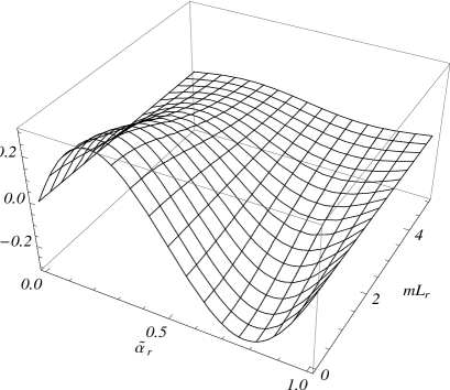
Figure 1: The VEV of fermionic current, $L_{r}^{4}\langle 0|j^{r}|0\rangle$, in the model with spatial topology $R^{3}\times S^{1}$ as a function of the phase $\tilde{\alpha}_{r}$ and the parameter $mL_{r}$.

3 Zeta function approach

In this section, for the evaluation of the VEV of fermionic current we follow a different route based on the zeta function method [7, 23, 24]. This allows us to obtain an alternative representation. To start we note that the mode sum for the fermionic current can be written as

$$\langle 0|j^{r}|0\rangle=\frac{\pi N}{L_{r}^{2}}\sum_{n_{r}=-\infty}^{+\infty}(n_{r}+\tilde{\alpha}_{r})\zeta(1/2),$$ (32)

where the generalized zeta function

$$\zeta(s)=\frac{L_{r}}{V_{q}}\int\frac{d\mathbf{k}_{p}}{(2\pi)^{p}}\sum_{\mathbf{n}_{q-1}^{r}\in\mathbf{Z}^{q-1}}\{\mathbf{k}_{p}^{2}+\sum_{l=p+1,\neq r}^{D}[2\pi(n_{l}+\tilde{\alpha}_{l})/L_{l}]^{2}+m_{r}^{2}\}^{-s},$$ (33)

is introduced with the notation

$$m_{r}^{2}=m^{2}+[2\pi(n_{r}+\tilde{\alpha}_{r})/L_{r}]^{2}.$$ (34)

As it follows from Eq. (32), for the evaluation of the renormalized VEV of fermionic current we need to have the analytic continuation of the zeta function $\zeta(s)$ at the point $s=1/2$.

With this aim we first integrate over the wave vector along the uncompactified dimensions:

$$\zeta(s)=\frac{\Gamma(s-p/2)L_{r}}{(4\pi)^{p/2}\Gamma(s)V_{q}}\sum_{\mathbf{n}_{q-1}^{r}\in\mathbf{Z}^{q-1}}\left\{\sum_{l=p+1,\neq r}^{D}[2\pi(n_{l}+\tilde{\alpha}_{l})/L_{l}]^{2}+m_{r}^{2}\right\}^{p/2-s}.$$ (35)

An exponentially convergent expression for the analytic continuation of the multiseries in Eq. (35) can be obtained by using the generalized Chowla-Selberg formula [25]. The application of this formula to Eq. (35) gives the following result

$$\zeta(s) = \frac{m_{r}^{D-2s-1}}{(4\pi)^{(D-1)/2}}\frac{\Gamma(s-(D-1)/2)}{\Gamma(s)}+\frac{2^{1-s}m_{r}^{D-2s-1}}{(2\pi)^{(D-1)/2}\Gamma(s)}$$ (36)

$$\times\sideset{}{{}^{\prime}}{\sum}_{\mathbf{n}_{q-1}^{r}\in\mathbf{Z}^{q-1}}\cos(2\pi\mathbf{n}_{q-1}^{r}\cdot\boldsymbol{\alpha}_{q-1})f_{(D-1)/2-s}(m_{r}g(\mathbf{L}_{q-1},\mathbf{n}_{q-1}^{r})),$$

with $\mathbf{L}_{q-1}=(L_{p+1},\ldots,L_{r-1},L_{r+1},\ldots L_{D})$ and $\boldsymbol{\alpha}_{q-1}=(\tilde{\alpha}_{p+1},\ldots,\tilde{\alpha}_{r-1},\tilde{\alpha}_{r+1},\ldots\tilde{\alpha}_{D})$. In Eq. (36) we have introduced the notation $f_{\nu}(x)=K_{\nu}(x)/x^{\nu}$. The prime on the summation sign in (36) means that the term $\mathbf{n}_{q}=0$ should be excluded from the sum and

$$g(\mathbf{L}_{q-1},\mathbf{n}_{q-1}^{r})=\Big{(}\sum_{i=p+1,\neq r}^{D}L_{i}^{2}n_{i}^{2}\Big{)}^{1/2}.$$ (37)

The part in the fermionic current containing the second term on the right-hand side of Eq. (36) is finite at the physical point and, hence, the analytic continuation is needed for the part with the first term alone. In order to do this, we apply the summation formula (19) to the corresponding series over $n_{r}$. After transformations similar to those already used in the derivation of Eq. (23) and by making use of the standard properties of the gamma function, one finds

$$\frac{\Gamma(s-(D-1)/2)}{2L_{r}(4\pi)^{(D-1)/2}\Gamma(s)}\sum_{n_{r}=-\infty}^{+\infty}\frac{2\pi(n_{r}+\tilde{\alpha}_{r})/L_{r}}{m_{r}^{2s+1-D}}$$

$$\quad=\frac{(2m)^{(D-2s)/2+1}}{(4\pi)^{D/2}\Gamma(s)}\sum_{n=1}^{\infty}\sin(2\pi n\tilde{\alpha}_{r})\frac{K_{(D-2s)/2+1}(nL_{r}m)}{(nL_{r})^{(D-2s)/2}}.$$ (38)

As it can be easily checked, the right-hand side of this relation is finite at $s=1/2$. Combining Eqs. (32), (36), (38), for the VEV of fermionic current we find the following representation

$$\langle 0|j^{r}|0\rangle = \frac{2Nm^{(D+1)/2}}{(2\pi)^{(D+1)/2}}\sum_{n=1}^{\infty}\sin(2\pi n\tilde{\alpha}_{r})\frac{K_{(D+1)/2}(nL_{r}m)}{(nL_{r})^{(D-1)/2}}+\frac{NL_{r}^{-2}}{(2\pi)^{D/2-1}}\sum_{n_{r}=-\infty}^{+\infty}(n_{r}+\tilde{\alpha}_{r})$$ (39)

$$\times m_{r}^{D-2}\sideset{}{{}^{\prime}}{\sum}_{\mathbf{n}_{q-1}^{r}\in\mathbf{Z}^{q-1}}\cos(2\pi\mathbf{n}_{q-1}^{r}\cdot\boldsymbol{\alpha}_{q-1})f_{D/2-1}(m_{r}g(\mathbf{L}_{q-1},\mathbf{n}_{q-1}^{r})).$$

Note that in the limit $L_{l}\rightarrow\infty$, $l\neq r$, the second term on the right-hand side of this formula vanishes and we obtain the vacuum fermionic current in the model with a single compact dimension. The latter coincides with Eq. (29).

Formula (39) is further simplified by using the relation

$$\sum_{n_{r}=-\infty}^{+\infty}\left[2\pi(n_{r}+\tilde{\alpha}_{r})/L_{r}\right]m_{r}^{D-2}f_{D/2-1}(m_{r}y)$$

$$\quad=\sqrt{\frac{2}{\pi}}L_{r}^{2}m^{D+1}\sum_{n_{r}=1}^{+\infty}n_{r}\sin(2\pi n_{r}\tilde{\alpha}_{r})f_{(D+1)/2}(m\sqrt{y^{2}+n_{r}^{2}L_{r}^{2}}).$$ (40)

This relation is obtained by integrating the Poisson’s resummation formula $\sum_{n=-\infty}^{+\infty}F(x)\delta(x-n)=\sum_{n=-\infty}^{+\infty}F(x)e^{2i\pi nx}$ with the function $F(x)$ defined by the left-hand side of Eq. (40). The integral for the right-hand side is evaluated using the formula from Ref. [22]. By taking into account Eq. (40), from Eq. (39) we find

$$\langle 0|j^{r}|0\rangle = \frac{2Nm^{D+1}L_{r}}{(2\pi)^{(D+1)/2}}\sum_{n_{r}=1}^{\infty}n_{r}\sin(2\pi n_{r}\tilde{\alpha}_{r})$$ (41)

$$\times\sum_{\mathbf{n}_{q-1}^{r}\in\mathbf{Z}^{q-1}}\cos(2\pi\mathbf{n}_{q-1}^{r}\cdot\boldsymbol{\alpha}_{q-1})f_{(D+1)/2}(mg(\mathbf{L}_{q},\mathbf{n}_{q})),$$

with the notation

$$g(\mathbf{L}_{q},\mathbf{n}_{q})=\Big{(}\sum_{i=p+1}^{D}L_{i}^{2}n_{i}^{2}\Big{)}^{1/2}.$$ (42)

The equivalence of two representations (23) and (41) for the VEV of fermionic current is seen using the relation

$$\sum_{\mathbf{n}_{q-1}^{r}\in\mathbf{Z}^{q-1}}\cos(2\pi\mathbf{n}_{q-1}^{r}\cdot\boldsymbol{\alpha}_{q-1})f_{(D+1)/2}(mg(\mathbf{L}_{q},\mathbf{n}_{q}))$$

$$\quad=\frac{(2\pi)^{(q-1)/2}L_{r}}{V_{q}m^{D+1}}\sum_{\mathbf{n}_{q-1}^{r}\in\mathbf{\ Z}^{q-1}}\omega_{\mathbf{n}_{q-1}^{r}}^{(D-q)/2+1}f_{(D-q)/2+1}(nL_{r}\omega_{\mathbf{n}_{q-1}^{r}}).$$ (43)

The proof of this relation can be found in Appendix of Ref. [16]. The advantage of the representation (23), as compared with Eq. (41), is that in the case of a massless field, for large values of $n_{l}$ the separate terms in the multiseries decay exponentially instead of power-law decay in Eq. (41).

4 Fermionic current in carbon nanotubes

Carbon nanotubes have attracted much attention recently due to the experimental observation of a number of novel electronic properties. In this section we apply general results obtained above for the electrons in cylindrical and toroidal carbon nanotubes. A single-wall cylindrical nanotube is a graphene sheet rolled into a cylindrical shape. The electronic band structure of graphene close to the Dirac points shows a conical dispersion $E(\mathbf{k})=v_{F}|\mathbf{k}|$, where $\mathbf{k}$ is the momentum measured relatively to the Dirac points and $v_{F}\approx 10^{8}$ cm/s represents the Fermi velocity which plays the role of a speed of light. The corresponding low-energy excitations can be described by a pair of two-component spinors, $\psi_{A}$ and $\psi_{B}$, corresponding to the two different triangular sublattices of the honeycomb lattice of graphene (see, for instance, [2, 3]). The Dirac equation for these spinors has the form

$$(iv_{F}^{-1}\gamma^{0}D_{0}+i\gamma^{l}D_{l}-m)\psi_{J}=0,\$$ (44)

where $J=A,B$, $l=1,2$, and $D_{\mu}$ is defined in Eq. (2) with $e=-|e|$ for electrons. To keep the discussion general we have included in Eq. (44) the mass (gap) term. The gap in the energy spectrum is essential in many physical application. This gap can be generated by a number of mechanisms (see, for example, [3, 26, 27, 28]). In particular, they include the breaking of symmetry between two sublattices by introducing a staggered onsite energy [3] and the deformations of bonds in the graphene lattice [26]. Another approach is to attach a graphene monolayer to a substrate the interaction with which breaks the sublattice symmetry [27]. For metallic nanotubes we have periodic boundary conditions ($\alpha_{l}=0$) along the compact dimension and for semiconductor nanotubes, depending on the chiral vector, we have two classes of inequivalent boundary conditions corresponding to $\alpha_{l}=\pm 1/3$. These phases have opposite signs for the sublattices $A$ and $B$.

The presence of the gauge field in Eq. (44) leads to the Aharonov-Bohm effect in carbon nanotubes [29]. This effect manifests itself in a periodic energy gap modulation and conductance oscillations as a function of enclosed magnetic flux with a period of the order of the flux quantum. Similar oscillations arise in the VEV of fermionic current along compact dimensions. We consider the cases of cylindrical and toroidal nanotubes separately.

4.1 The case $D=1$

We start with the simplest case $D=1$ with a compact dimension of the length $L_{1}=L$. The corresponding phase in the periodicity condition we denote $\alpha_{1}=\alpha$. As it is seen below, this case can be considered as a model of a toroidal nanotube in the limit when the length of the one of compact dimensions is small. The corresponding effective two-dimensional Dirac-like theory is discussed in Refs. [30]. By summing the contributions coming from two sublattices with opposite signs of $\alpha$, for the VEV of fermionic current one finds

$$\langle j^{1}\rangle=\frac{4v_{F}m}{\pi}\sum_{n=1}^{\infty}\cos(2\pi n\alpha)\sin(2\pi n\Phi/\Phi_{0})K_{1}(mLn),$$ (45)

where $2\pi\Phi/\Phi_{0}=eA_{1}L/(\hbar c)$ with $\Phi$ being the magnetic flux. The corresponding vector potential can be generated by the magnetic field perpendicular to the plane of torus and located inside a coaxial cylinder with radius smaller than $L/(2\pi)$. For a massless case from here we have $\langle j^{1}\rangle=v_{F}\sum_{j=\pm}\mathcal{I}(\Phi/\Phi_{0}+j\alpha)/L$, where we have defined the function

$$\mathcal{I}(x)=\frac{2}{\pi}\sum_{n=1}^{\infty}\frac{\sin(2\pi nx)}{n}=\left\{\begin{array}[]{cc}1-2\{x\},&\{x\}>0\\ 2|\{x\}|-1,&\{x\}<0\end{array}\right..$$ (46)

The fractional part $\{x\}$ on the right-hand side of this formula is defined in accordance with the Mathematica function FractionalPart[$x$]. In figure 2 we have plotted the VEV (45) as a function of the magnetic flux for different values of the parameter $mL$ (numbers near the curves). The dashed lines correspond to a massless case. For the left and right panels $\alpha=0$ and $\alpha=1/3$, respectively. The electric current corresponding to the VEV of the fermionic current is of order $|e|v_{F}/L$. Note that the persistent currents in normal metal rings with this order of magnitude have been recently measured in Refs. [31].

Figure 2: The VEV of fermionic current in $D=1$ model for the periodicity conditions with $\alpha=0$ (left panel) and $\alpha=1/3$ (right panel) as a function of the magnetic flux.

4.2 Cylindrical nanotubes

A single-wall cylindrical nanotube is a rolled-up graphene sheet in the hollow cylindrical structure. For the case of cylindrical nanotube we have spatial topology $R^{1}\times S^{1}$ with the compactified dimension of length $L$. The nanotube is characterized by its chiral vector $\mathbf{C}_{h}=(n_{w},m_{w})$, with $n_{w}$, $m_{w}$ being integers determining the circumference in accordance with $L=|\mathbf{C}_{h}|=a\sqrt{n_{w}^{2}+m_{w}^{2}+n_{w}m_{w}}$. Here $a=2.46\mathring{A}$ is the lattice constant for graphene. A zigzag nanotube corresponds to the special case $\mathbf{C}_{h}=(n_{w},0)$, and a armchair nanotube corresponds to the case $\mathbf{C}_{h}=(n_{w},n_{w})$. All other cases correspond to chiral nanotubes. The electronic properties of carbon nanotubes can be either metallic or semiconductor-like depending on the chiral vector. In the case $n_{w}-m_{w}=3q_{w}$, $q_{w}\in Z$, the nanotube will be metallic and in the case $n_{w}-m_{w}\neq 3q_{w}$ the nanotube will be semiconductor with an energy gap inversely proportional to the diameter.

For the case under discussion $D=2$ and the general formula for the VEV of fermionic current takes the form ($N=2$, $\alpha_{p+1}\equiv\alpha$)

$$\langle 0|j^{2}|0\rangle=\frac{1}{\pi L^{2}}\sum_{n=1}^{\infty}\sin(2\pi n\tilde{\alpha})\frac{1+nLm}{n^{2}e^{nLm}},$$ (47)

with the notation $\tilde{\alpha}=\alpha+eA_{2}L/(2\pi)$, and $\langle 0|j^{1}|0\rangle=0$. In metallic nanotubes $\alpha=0$ and for semiconductor nanotubes $\alpha=\pm 1/3$. For graphene sheet we have two spinors that describe Bloch states residing on the two different sublattices. Summing the contributions from these sublattices and taking into account that, for these two sublattices the phases $\alpha$ have opposite signs, for the total fermionic current we find

$$\langle j^{2}\rangle^{\text{(cn)}}=\frac{2v_{F}}{\pi L^{2}}\sum_{n=1}^{\infty}\cos(2\pi n\alpha)\sin(2\pi n\Phi/\Phi_{0})\frac{1+nLm}{n^{2}e^{nLm}},$$ (48)

where $\alpha=0,1/3$ for metallic and semiconductor nanotubes respectively. In these formulae $2\pi\Phi/\Phi_{0}=eA_{2}L/(\hbar c)$ with $\Phi$ being the magnetic flux passing through the cross section of the nanotube. Note that in Eq. (48) (and in the formulae below), we give the fermionic current for a given spin component. The total current is obtained multiplying by the number of spin components which is 2 for graphene.

As it is seen from Eq. (48), in the absence of the magnetic flux the total fermionic current vanishes due to the cancellation of contributions from two sublattices. The magnetic flux breaks this symmetry and an effective current appears. However, it should be noted that, in general, the mass terms in the Dirac equation for separate sublattices can be different. In this case an effective fermionic current appears without an external magnetic field. In figure 3 we plot the VEV of the fermionic current for various values of the parameter $mL$ (numbers near the curves) in metallic (left panel) and semiconductor (right panel) cylindrical nanotubes as a function of magnetic flux in units of magnetic flux quantum.

Figure 3: The VEV of fermionic current in metallic (left panel) and semiconductor (right panel) nanotubes as a function of the magnetic flux.

4.3 Toroidal nanotubes

A toroidal nanotube corresponds to a finite graphene sheet with the periodical boundary conditions along the transverse and longitudinal directions. This form of carbon structure was discovered in Refs. [5]. The carbon toroid is determined by its chiral, $\mathbf{C}_{h}=(n_{w},m_{w})$, and translational, $\mathbf{T}=(p_{w},q_{w})$, vectors. The parameters $(n_{w},m_{w},p_{w},q_{w})$ define the geometric structure and physical properties of toroidal nanotubes. For the geometry of a toroidal nanotube we have the spatial topology $(S^{1})^{2}$ with $p=0$ and $q=2$ and the corresponding formulae for the VEV of fermionic current are directly obtained from the general results (23) and (41) (on the persistent currents in toroidal carbon nanotubes see Refs. [32]). For a graphene sheet we have two sublattices with opposite signs of the phases $\alpha_{l}$. The total current is obtained by summing the corresponding contributions and one finds

$$\langle j^{r}\rangle^{\text{(tor)}} = \frac{2L_{r}v_{F}}{\pi}\sum_{n_{r}=1}^{\infty}n_{r}\sum_{n_{l}=-\infty}^{\infty}\frac{\cos[2\pi\left(n_{1}\alpha_{1}+n_{2}\alpha_{2}\right)]}{(L_{1}^{2}n_{1}^{2}+L_{2}^{2}n_{2}^{2})^{3/2}}$$ (49)

$$\times\frac{1+m\sqrt{L_{1}^{2}n_{1}^{2}+L_{2}^{2}n_{2}^{2}}}{\exp(m\sqrt{L_{1}^{2}n_{1}^{2}+L_{2}^{2}n_{2}^{2}})}\sin\left[2\pi\left(n_{1}\Phi_{1}+n_{2}\Phi_{2}\right)/\Phi_{0}\right],$$

where $r,l=1,2,$ $l\neq r$, and $2\pi\Phi_{l}/\Phi_{0}=eA_{l}L_{l}/(\hbar c)$. As in the case of cylindrical nanotubes, due to the cancellation of contributions coming from separate sublattices, the fermionic current in toroidal nanotubes vanishes in the absence of the magnetic flux. An alternative representation is obtained by using formula (23):

$$\langle j^{r}\rangle^{\text{(tor)}} = \frac{2v_{F}}{\pi L_{l}^{2}}\sum_{\delta=\pm}\sum_{n_{r}=1}^{\infty}\sin(2\pi n_{r}\tilde{\alpha}_{r}^{(\delta)})\sum_{n_{l}=-\infty}^{+\infty}\sqrt{[2\pi(n_{l}+\tilde{\alpha}_{l}^{(\delta)})]^{2}+L_{l}^{2}m^{2}}$$ (50)

$$\times K_{1}(n_{r}(L_{r}/L_{l})\sqrt{[2\pi(n_{l}+\tilde{\alpha}_{l}^{(\delta)})]^{2}+L_{l}^{2}m^{2}}),$$

with $r,l=1,2,$ $l\neq r$, and $\tilde{\alpha}_{l}^{(\pm)}=\pm\alpha_{l}+\Phi_{l}/\Phi_{0}$. This formula is further simplified when $A_{l}=0$:

$$\langle j^{r}\rangle^{\text{(tor)}} = \frac{4v_{F}}{\pi L_{l}^{2}}\sum_{n=1}^{\infty}\sin(2\pi n_{r}\Phi_{r}/\Phi_{0})\cos(2\pi n_{r}\alpha_{r})\sum_{n_{l}=-\infty}^{+\infty}\sqrt{[2\pi(n_{l}+\alpha_{l})]^{2}+L_{l}^{2}m^{2}}$$ (51)

$$\times K_{1}(n_{r}(L_{r}/L_{l})\sqrt{[2\pi(n_{l}+\alpha_{l})]^{2}+L_{l}^{2}m^{2}}).$$

Note that in this case the component $\langle 0|j^{l}|0\rangle^{\text{(tor)}}$ is nonzero only for $\alpha_{1},\alpha_{2}\neq 0$.

Let us consider the asymptotic limit of the fermionic current in toroidal nanotubes in the case $L_{1}\ll L_{2}$ for a fixed value of $mL_{2}$. First we consider the component $\langle j^{1}\rangle^{\text{(tor)}}$. For this component in Eq. (50) one has $l=2$. In the limit under consideration the main contribution to the series over $n_{2}$ comes from large values and we can replace the summation by integration. The integral is evaluated explicitly and to the leading order the expression for $\langle j^{1}\rangle^{\text{(tor)}}$ coincides with the corresponding result for cylindrical nanotubes given by (48) (with $L=L_{1}$). The behavior of the component $\langle j^{2}\rangle^{\text{(tor)}}$ crucially depends on whether the parameter $\tilde{\alpha}_{1}^{(\delta)}$ is integer or not. When this parameter is non-integer (for both $\delta=\pm$) the argument of the modified Bessel function in Eq. (51) (with $r=2$, $l=1$) is large and the dominant contribution comes from the term with $n_{2}=1$ and from the term in the summation over $n_{1}$ with minimum value of $|n_{1}+\tilde{\alpha}_{1}^{(\delta)}|$. The VEV of fermionic current is exponentially suppressed: $\langle j^{2}\rangle^{\text{(tor)}}\sim\exp[-\sqrt{(2\pi\beta_{1}L_{2}/L_{1})^{2}+L_{2}^{2}m^{2}}]$, with $\beta_{1}=\min|n_{1}+\tilde{\alpha}_{1}^{(\delta)}|$. For nanotubes metallic along the direction $z^{1}$ with the length $L_{1}$ and for $A_{1}=0$ one has $\tilde{\alpha}_{1}^{(\pm)}=0$. In this case and for $L_{1}\ll L_{2}$ the main contribution to $\langle j^{2}\rangle^{\text{(tor)}}$ comes from the term with $n_{1}=0$ in Eq. (50) and the quantity $L_{1}\langle j^{2}\rangle^{\text{(tor)}}$ coincides with the corresponding result in $D=1$ case (formula (45) with $L=L_{2}$ and $\alpha=\alpha_{2}$). If $\alpha_{1}\neq 0$ and $\tilde{\alpha}_{1}^{(\delta)}$ is an integer (note that this can be satisfied for one of values $\delta$) the main contribution comes from the term for which $n_{1}+\tilde{\alpha}_{1}^{(\delta)}=0$. In this case only one of the sublattices contributes to the fermionic current.

In figure 4 we plot the dependence of the fermionic current $\langle j^{2}\rangle^{\text{(tor)}}$ in the massless case as a function of the ratio $L_{1}/L_{2}$ for different values of the phases $(\alpha_{1},\alpha_{2})$ (numbers near the curves) and for $\Phi_{2}/\Phi_{0}=0.2$, $\Phi_{1}=0$. In this case the component $\langle j^{1}\rangle^{\text{(tor)}}$ is nonzero for $\alpha_{1,2}\neq 0$ only. As it was shown above and clearly seen from figure, for large values of the ratio $L_{1}/L_{2}$ the component $\langle j^{2}\rangle^{\text{(tor)}}$ of the fermionic current tends to the corresponding quantity in a cylindrical nanotube with circumference $L_{2}$. In the opposite limit of small values of $L_{1}/L_{2}$ the VEV tends to zero for semiconducting type periodicity condition along the direction $z^{1}$. Again, this is in agreement with the asymptotic analysis given before.

Figure 4: The VEV of the current for a massless fermionic field in a toroidal nanotube as a function of the ratio $L_{1}/L_{2}$ for different values of the phases $(\alpha_{1},\alpha_{2})$ and for the magnetic flux $\Phi_{2}/\Phi_{0}=0.2$, $\Phi_{1}=0$.

The dependence of the fermionic current on the magnetic flux is presented in figure 5 for different values of the ratio $L_{1}/L_{2}$. The left and right panels correspond to toroidal nanotubes with phases $(\alpha_{1},\alpha_{2})=(1/3,0)$ and $(1/3,1/3)$, respectively.

Figure 5: The VEV of fermionic current in the massless case for toroidal nanotubes with $(\alpha_{1},\alpha_{2})=(1/3,0)$ (left panel) and $(\alpha_{1},\alpha_{2})=(1/3,1/3)$ (right panel) as a function of the magnetic flux for various values of the ratio $L_{1}/L_{2}$.

5 Conclusion

We have investigated the VEV of fermionic current for a massive spinor field in the background of flat spacetime with spatial topology $R^{p}\times S^{q}$. Along the compact dimensions the field obeys generic quasiperiodic boundary conditions (1). In addition, we have assumed the presence of a constant gauge field. For the evaluation of the mode sum of the fermionic current two different approaches have been used. They give two alternative representations of the vacuum current. In the first approach, we apply to the mode sum the Abel-Plana type summation formula (19). The renormalized VEV of fermionic current components along compact dimensions is given by formula (23). The time component and the components along the uncompactified dimensions vanish. The fermionic current depends on the phases in the periodicity conditions and on the gauge potential in the combination (18). It is a periodic function of the magnetic flux with the period of the flux quantum. In order to obtain an alternative representation of the vacuum current, in Section 3 we have followed the zeta function approach. An exponentially convergent expression for the analytic continuation of the corresponding mode-sum is obtained on the basis of the generalized Chowla-Selberg formula. The corresponding expression for the components of fermionic current along compact dimensions is given by Eq. (41). The equivalence of two representations for the VEV of the fermionic current is directly seen by using the relation (40). As a numerical example, in figure 1 we have depicted the dependence of the vacuum current in the 5-dimensional Kaluza-Klein model on the phases in the periodicity conditions and on the mass of the field. In this type models the fermionic current with the components along compact dimensions is a source of cosmological magnetic fields.

In Section 4 we gave an application of the general results to the electrons of a graphene sheet rolled into cylindrical and toroidal shapes. For the description of relevant low-energy degrees of freedom we have followed a route based on the effective field theory treatment of graphene in terms of a pair of Dirac fermions. For this model we have $D=2$ and the topologies $R^{1}\times S^{1}$ and $(S^{1})^{2}$ for cylindrical and toroidal nanotubes, respectively. Depending on the manner the cylinder is obtained from the graphene sheet, the phases in the periodicity conditions for the fields are equal to $0$ for metallic nanotubes and to $\pm 1/3$ for semiconductor ones. These phases have opposite signs for the two sublattices of the hexagonal lattice of graphene. In cylindrical nanotubes the total fermionic current is given by formula (48). In the absence of magnetic flux, the total fermionic current vanishes due to the cancellation of contributions from two sublattices. For toroidal nanotubes the two equivalent representations for the VEV of fermionic current are given by Eqs. (49) and (50). As in the case of cylindrical nanotubes, due to the cancellation of contributions coming from separate sublattices, the fermionic current vanishes in the absence of magnetic flux. However, the mass terms for two sublattices can be different and in this case an effective fermionic current appears in the absence of the magnetic flux.

In a way similar to that used in this paper, we can investigate the effects of non-trivial topology on the VEV of axial current in even dimensional spacetimes. It is well-known that in external electromagnetic and gravitational fields the chiral anomaly appears in the divergence of the axial current (for a review see [33]). However, in the problem under consideration these anomalies are absent as the spacetime is flat and the electromagnetic field tensor vanishes.

References

- [1] A. Linde, JCAP 10, 004 (2004).
- [2] R. Saito, G. Dresselhaus, and M. S. Dresselhaus, Physical Properties of Carbon Nanotubes (Imperial College Press, London, 1998); C. Dupas, P. Houdy, and M. Lahmani (Editors), Nanoscience: Nanotechnologies and Nanophysics (Springer, Berlin, 2007).
- [3] G.W. Semenoff, Phys. Rev. Lett. 53, 2449 (1984).
- [4] D.P. Di Vincenzo and E.J. Mele, Phys. Rev. B 29, 1685 (1984); J. Gonzàlez, F. Guinea, and M.A.H. Vozmediano, Nucl. Phys. B 406, 771 (1993); Phys. Rev. B 63, 134421 (2001); H.-W. Lee and D.S. Novikov, Phys. Rev. B 68, 155402 (2003); S.G. Sharapov, V.P. Gusynin, and H. Beck, Phys. Rev. B 69, 075104 (2004); K.S. Novoselov et al, Nature 438, 197 (2005); D. S. Novikov and L. S. Levitov, Phys. Rev. Lett. 96, 036402 (2006); E. Perfetto, J. González, F. Guinea, S. Bellucci, and P. Onorato, Phys. Rev. B 76, 125430 (2007); A.H. Castro Neto, F. Guinea, N.M.R. Peres, K.S. Novoselov, and A.K. Geim, Rev. Mod. Phys. 81, 109 (2009).
- [5] H. Liu, H. Dai, J.H. Hafner, D.T. Colbert, R.E. Smalley, S.J. Tans, and C. Dekker, Nature 385, 780 (1997); R. Martel, H.R. Shea, and P. Avouris, Nature 398, 299 (1999).
- [6] V.M. Mostepanenko and N.N. Trunov, The Casimir Effect and Its Applications (Clarendon, Oxford, 1997).
- [7] E. Elizalde, S.D. Odintsov, A. Romeo, A.A. Bytsenko and S. Zerbini, Zeta regularization techniques with applications (World Scientific, Singapore, 1994).
- [8] K.A. Milton, The Casimir Effect: Physical Manifestation of Zero-Point Energy (World Scientific, Singapore, 2002).
- [9] M. Bordag, G.L. Klimchitskaya, U. Mohideen, and V.M. Mostepanenko, Advances in the Casimir Effect (Oxford University Press, Oxford, 2009).
- [10] M.J. Duff, B.E.W. Nilsson, and C.N. Pope, Phys. Rep. 130, 1 (1986); A.A. Bytsenko, G. Cognola, L. Vanzo, and S. Zerbini, Phys. Rep. 266, 1 (1996).
- [11] G.L. Klimchitskaya, U. Mohidden, and V.M. Mostepanenko, Rev. Mod. Phys. 81, 1827 (2009).
- [12] K.A. Milton, Grav. Cosmol. 9, 66 (2003); E. Elizalde, S. Nojiri, and S.D. Odintsov, Phys. Rev D 70, 043539 (2004); E. Elizalde, J. Phys. A 39, 6299 (2006); B. Greene and J. Levin, J. High Energy Phys. 0711, 096 (2007); P. Burikham, A. Chatrabhuti, P. Patcharamaneepakorn, and K. Pimsamarn, J. High Energy Phys. 0807, 013 (2008).
- [13] J.S. Dowker and R. Critchley, J. Phys. A: Math. Gen. 9, 535 (1976); R. Banach and J.S. Dowker, J. Phys. A: Math. Gen. 12, 2545 (1979); B.S. DeWitt, C.F. Hart, and C.J. Isham, Physica A 96, 197 (1979); S.G. Mamayev and N.N. Trunov, Russian Phys. J. 22, 766 (1979); 23, 551 (1980); L.H. Ford, Phys. Rev. D 21, 933 (1980); J. Ambjørn and S. Wolfram, Ann. Phys. 147, 1 (1983); S.G. Mamayev and V.M. Mostepanenko, In Proceedings of the Third Seminar on Quantum Gravity (World Scientific, Singapore, 1985); Yu.P. Goncharov and A.A. Bytsenko, Phys. Lett. B 160, 385 (1985); Yu.P. Goncharov and A.A. Bytsenko, Nucl. Phys. B 271, 726 (1986); Yu.P. Goncharov and A.A. Bytsenko, Class. Quant. Grav. 4, 555 (1987); E. Elizalde, Z. Phys. C 44, 471 (1989); E. Ponton and E. Poppitz, JHEP 0106, 019 (2001); H. Queiroz, J.C. da Silva, F.C. Khanna, J.M.C. Malbouisson, M. Revzen, and A.E. Santana, Ann. Phys. 317, 220 (2005); A.A. Saharian and M.L. Mkhitaryan, Eur. Phys. J. C, in press, arXiv:0911.1260.
- [14] A.A. Saharian and M. R. Setare, Phys. Lett. B 659, 367 (2008); S. Bellucci and A. A. Saharian, Phys. Rev. D 77, 124010 (2008).
- [15] A.A. Saharian, Class. Quantum Grav. 25, 165012 (2008); E.R. Bezerra de Mello and A.A. Saharian, JHEP 0812, 081 (2008).
- [16] S. Bellucci and A.A. Saharian, Phys. Rev. D 79, 085019 (2009).
- [17] S. Bellucci and A.A. Saharian, Phys. Rev. D 80, 105003 (2009).
- [18] V.B. Bezerra and E.R. Bezerra de Mello, Class. Quantum Grav. 11, 457 (1994); E.R. Bezerra de Mello, Class. Quantum Grav. 11, 1415 (1994); L. Sriramkumar, Class. Quantum Grav. 18, 1015 (2001); E.R. Bezerra de Mello, arXiv:0907.4139; Yu.A. Sitenko and N.D. Vlasii, Class. Quantum Grav. 26, 195009 (2009).
- [19] E. R. Bezerra de Mello and A. A. Saharian, Phys. Rev. D 78, 045021 (2008).
- [20] S.G. Mamayev, V.M. Mostepanenko, and A.A. Starobinsky, Sov. Phys. JETP 43, 823 (1976) [Zh. Eksp. Teor. Fiz. 70, 1577 (1976)].
- [21] A. A. Saharian, The Generalized Abel-Plana Formula with Applications to Bessel Functions and Casimir Effect (Yerevan State University Publishing House, Yerevan, 2008); Preprint ICTP/2007/082; arXiv:0708.1187.
- [22] A.P. Prudnikov, Yu.A. Brychkov, and O.I. Marichev, Integrals and Series (Gordon and Breach, New York, 1986), Vol. 2.
- [23] E. Elizalde, Ten Physical Applications of Spectral Zeta Functions, Lecture Notes in Physics (Springer-Verlag, Berlin, 1995);
- [24] K. Kirsten, Spectral Functions in Mathematics and Physics (CRC Press, Boca Raton, FL, 2001).
- [25] E. Elizalde, Commun. Math. Phys. 198, 83 (1998); E. Elizalde, J. Phys. A: Math. Gen. 34, 3025 (2001).
- [26] C. Chamon, Phys. Rev. B 62, 2806 (2000); C.-Y. Hou, C. Chamon, and C. Mudry, Phys. Rev. Lett. 98, 186809 (2007).
- [27] G. Giovannetti, P.A. Khomyakov, G. Brocks, P.J. Kelly, and J. van den Brink, Phys. Rev. B 76, 073103 (2007); S.Y. Zhou et al., Nature Mater. 6, 770 (2007).
- [28] G.W. Semenoff, V. Semenoff, and F. Zhou, Phys. Rev. Lett. 101, 087204 (2008).
- [29] H. Ajiki and T. Ando, J. Phys. Soc. Jpn. 62, 1255 (1993); Physica B 201, 349 (1994); A. Bachtold et al., Nature 397, 673 (1999); S. Zaric et al., Science 304, 1129 (2004); U.S. Coskun et al., Science 304, 1132 (2004); J. Cao, Q. Wang, M. Rolandi, and H. Dai, Phys. Rev. Lett. 93, 216803 (2004); B. Lassagne et al., Phys. Rev. Lett. 98, 176802 (2007); M.-G. Kang et al., Phys. Rev. B 77, 113408 (2008).
- [30] K. Sasaki, Phys. Lett. A 296, 237 (2002); K. Sasaki, Phys. Rev. B 65, 155429 (2002).
- [31] H. Bluhm et al., Phys. Rev. Lett. 102, 136802 (2009); A.C. Bleszynski-Jayich et al., Science 326, 272 (2009).
- [32] M.F. Lin and D.S. Chuu, Phys. Rev. B 57, 6731 (1998); M. Marganska and M. Szopa, Acta Phys. Pol. B 32, 427 (2001); S. Latil, S. Roche, and A. Rubio, Phys. Rev. B 67, 165420 (2003); R. B. Chen et al., Carbon 42, 2837 (2004); K. Sasaki and Y. Kawazoe, Prog. Theor. Phys. 112, 369 (2004); Z. Zhang, J. Yuan, M. Qiu, J. Peng, and F. Xiao, J. Appl. Phys. 99, 104311 (2006); N. Xu, J.W. Ding, H.B. Chen, and M.M. Ma, Eur. Phys. J. B 67, 71 (2009).
- [33] S.B. Treiman, R. Jackiw, and D.J. Gross, Lectures on Current Algebra and Its Applications (Princeton University Press, Princeton, 1972); F. Bastianelli and P. Van Nieuwenhuizen, Path Integrals and Anomalies in Curved Space (Cambridge University Press, Cambridge, 2006).