∎
22email: luigi.brugnano@unifi.it 33institutetext: Felice Iavernaro 44institutetext: Dipartimento di Matematica, Università di Bari, Via Orabona 4, 70125 Bari (Italy).
44email: felix@dm.uniba.it 55institutetext: Donato Trigiante 66institutetext: Dipartimento di Energetica, Università di Firenze, Via Lombroso 6/17, 50134 Firenze (Italy).
66email: trigiant@unifi.it
Isospectral Property of Hamiltonian Boundary Value Methods (HBVMs) and their blended implementation††thanks: Work developed within the project “Numerical methods and software for differential equations”.
Abstract
One main issue, when numerically integrating autonomous Hamiltonian systems, is the long-term conservation of some of its invariants, among which the Hamiltonian function itself. Recently, a new class of methods, named Hamiltonian Boundary Value Methods (HBVMs) has been introduced and analysed BIT , which are able to exactly preserve polynomial Hamiltonians of arbitrarily high degree. We here study a further property of such methods, namely that of having, when cast as Runge-Kutta methods, a matrix of the Butcher tableau with the same spectrum (apart the zero eigenvalues) as that of the corresponding Gauss-Legendre method, independently of the considered abscissae. Consequently, HBVMs are always perfectly -stable methods. Moreover, this allows their efficient blended implementation, for solving the generated discrete problems.
Keywords:
polynomial Hamiltonian energy preserving methods extended collocation methods Hamiltonian Boundary Value Methods HBVMs block Boundary Value Methods blended implicit methods Runge-Kutta methods blended iterationMSC:
65P10 65L05 65L06 65L80 65H101 Introduction
Hamiltonian problems are of great interest in many fields of application, ranging from the macro-scale of celestial mechanics, to the micro-scale of molecular dynamics. They have been deeply studied, from the point of view of the mathematical analysis, since two centuries. Their numerical solution is a more recent field of investigation, which has led to define symplectic methods, i.e., the simplecticity of the discrete map, considering that, for the continuous flow, simplecticity implies the conservation of . However, the conservation of the Hamiltonian and simplecticity of the flow cannot be satisfied at the same time unless the integrator produces the exact solution (see (HLW, , page 379)). More recently, the conservation of energy has been approached by means of the definition of the discrete line integral, in a series of papers IP1 ; IP2 ; IT1 ; IT2 ; IT3 , leading to the definition of Hamiltonian Boundary Value Methods (HBVMs) BIS ; BIT2 ; BIT ; BIT1 , which are a class of methods able to preserve, for the discrete solution, polynomial Hamiltonians of arbitrarily high degree (and then, a practical conservation of any sufficiently differentiable Hamiltonian). In more details, in BIT , HBVMs based on Lobatto nodes have been analysed, whereas in BIT1 HBVMs based on Gauss-Legendre abscissae have been considered. In the last reference, it has been actually shown that both formulae are essentially equivalent to each other, in the sense that they share the same order (twice the number of fundamental stages) and stability properties, and both methods provide the very same numerical solution, when the number of the so called silent stages tends to infitiny.111Actually, they both provide the same numerical solution also when the Hamiltonian is a polynomial and the number of silent stages is high enough to ensure the conservation property of the Hamiltonian function itself (see (2)). In this paper this conclusion if further supported, since we prove that all such methods, when cast as Runge-Kutta methods, have the corresponding matrix of the tableau, whose nonzero eigenvalues coincide with those of the corresponding Gauss-Legendre formula (isospectral property of HBVMs).
This property can be used to define an efficient iteration for solving the discrete problems generated by the methods, via their blended implementation. Indeed, after posing HBVMs in block BVM form, they can be recast in the framework of blended implicit methods, which have been studied in a series of papers B00 ; BM02 ; BM04 ; BM07 ; BM08 ; BM09 ; BM09a ; BMM06 ; BT2 (see also C. Magherini’s PhD Thesis M04 ). The latter methods have been successfully implemented in the two computational codes BiM and BiMD BIMcode ; the latter code is also included in the current release of the “Test Set for IVP Solvers” TestSet .
With this premise, the structure of the paper is the following: in Section 2 the basic facts about HBVMs are recalled; in Section 3 we state the main result of this paper, concerning the isospectral property; in Section 4 the discrete problem to be actually solved is defined; in Section 5 it is shown that a corresponding blended iteration can be devised for its efficient solution, which can be tuned by choosing a free parameter; in Section 6 the optimal choice of the free parameter is done, on the basis of the isospectral property of HBVM, by using a linear analysis of convergence; finally, in Section 7 a few concluding remarks are given.
2 Hamiltonian Boundary Value Methods
The arguments in this section are worked out starting from the arguments used in BIT ; BIT1 to introduce and analyse HBVMs. We consider canonical Hamiltonian problems in the form
| (1) |
where is a skew-symmetric constant matrix, and the Hamiltonian is assumed to be sufficiently differentiable. The key formula which HBVMs rely on, is the line integral and the related property of conservative vector fields:
| (2) |
for any , where is any smooth function such that
| (3) |
Here we consider the case where is a polynomial of degree , yielding an approximation to the true solution in the time interval . The numerical approximation for the subsequent time-step, , is then defined by (3).
After introducing a set of distinct abscissae
| (4) |
we set
| (5) |
so that may be thought of as an interpolation polynomial, interpolating the fundamental stages , , at the abscissae (4). We observe that, due to (3), also interpolates the initial condition .
Remark 1
Let us consider the following expansions of and for :
| (6) |
where is a suitable basis of the vector space of polynomials of degree at most and the (vector) coefficients are to be determined. We shall consider an orthonormal basis of polynomials on the interval , i.e.:
| (7) |
where is the Kronecker symbol, and has degree . Such a basis can be readily obtained as
with the shifted Legendre polynomial, of degree , on the interval .
Remark 2
We shall also assume that is a polynomial, which implies that the integrand in (2) is also a polynomial so that the line integral can be exactly computed by means of a suitable quadrature formula. It is easy to observe that in general, due to the high degree of the integrand function, such quadrature formula cannot be solely based upon the available abscissae : one needs to introduce an additional set of abscissae , distinct from the nodes , in order to make the quadrature formula exact:
where , , and , , denote the weights of the quadrature formula corresponding to the abscissae , i.e.,
Remark 3
According to IT2 , the right-hand side of (2) is called discrete line integral, while the vectors
| (10) |
are called silent stages: they just serve to increase, as much as one likes, the degree of precision of the quadrature formula, but they are not to be regarded as unknowns since, from (6) and (10), they can be expressed in terms of linear combinations of the fundamental stages (5).
Definition 1
In the sequel, we shall see that HBVMs may be expressed through different, though equivalent, formulations: some of them can be directly implemented in a computer program, the others being of more theoretical interest.
Because of the equality (2), we can apply the procedure directly to the original line integral appearing in the left-hand side. With this premise, by considering the first expansion in (6), the conservation property reads
which, as is easily checked, is certainly satisfied if we impose the following set of orthogonality conditions:
| (11) |
Then, from the second relation of (6) we obtain, by introducing the operator
that is the eigenfunction of relative to the eigenvalue :
| (13) |
Remark 4
Some further details are in order to better elucidate the role of the MFE in devising our methods. First of all we observe that, by definition, the MFE intrinsically brings, with its polynomial solutions , the conservation property of the Hamiltonian function: indeed (13) is equivalent to (2) under the choice (11).
This means that, when searching for its solutions, one should always take care of the precise dimension of the polynomial vector space, say , is intended to belong to: the higher is , the higher must be the number of silent stages (and hence the number of steps ) to guarantee that (2) be satisfied. This explains the way the solutions of the MFE depends on .
It is also clear that, assuming the same kind of distribution for all the the nodes (see later), (2) will be satisfied starting from a suitable number of steps on. This implies that, for all , HBVM will define the same polynomial of degree , such that .
where
Inserting (11) into (14) yields the final formulae which define the HBVMs class based upon the orthonormal basis :
| (15) |
We recall once again that we are working under the assumption (2), namely that the Hamiltonian is a polynomial and that we are considering a sufficient number of additional abscissae such that the line integral and its discrete counterpart do coincide. This implies that we can replace the integrals appearing in (15) by sums representing the associated quadrature formulae introduced in (2), without introducing any discretization error.
This leads back to express the HBVM method in terms of the fundamental stages and the silent stages (see (10)). By using the notation
| (16) |
we obtain
| (17) |
We again stress that the silent stages may be removed from (17) by observing that, for example,
where are the cardinal Lagrange polynomials defined on the nodes , .
From the above discussion it is clear that formulae (15) also make sense in the non-polynomial case. In fact, supposing to choose the abscissae so that the sums in (17) converge to an integral as , the resulting formula is again (15).
This implies that HBVMs may be as well applied in the non-polynomial case since, in finite precision arithmetic, HBVMs are undistinguishable from their limit formulae (15), when a sufficient number of silent stages is introduced. The aspect of having a practical exact integral, for large enough, was already stressed in BIS ; BIT ; BIT1 ; IP1 ; IT2 .
2.1 Runge-Kutta formulation of HBVMs
On the other hand, we emphasize that, in the non-polynomial case, (15) becomes an operative method only after that a suitable strategy to approximate the integrals appearing in it is taken into account. In the present case, if one discretizes the Master Functional Equation (2)–(13), HBVM are then obtained, essentially by extending the discrete problem (17) also to the silent stages (10). In order to simplify the exposition, we shall use (16) and introduce the following notation:
The discrete problem defining the HBVM then becomes,
| (18) |
By introducing the vectors
and the matrices
| (19) |
whose th entry are given by
| (20) |
we can cast the set of equations (18) in vector form as
with an obvious meaning of . Consequently, the method can be seen as a Runge-Kutta method with the following Butcher tableau:
| (21) |
Remark 5
We observe that, because of the use of an orthonormal basis, the role of the abscissae and of the silent abscissae is interchangeable, within the set . This is due to the fact that all the matrices , , and depend on all the abscissae , and not on a subset of them, and they are invariant with respect to the choice of the fundamental abscissae .
Hereafter, we shall consider a Gauss distribution of the abscissae , so that the resulting HBVM method BIT1 :
-
•
has order for all ;
-
•
is symmetric and perfectly -stable (i.e., its stability region coincides with the left-half complex plane, BT );
-
•
reduces to the Gauss-Legendre method of order , when ;
-
•
exactly preserves polynomial Hamiltonian functions of degree , provided that
3 The Isospectral Property
We are now going to prove a further additional result, related to the matrix appearing in the Butcher tableau (21), corresponding to HBVM, i.e., the matrix
| (22) |
whose rank is . Consequently it has a -fold zero eigenvalue. In this section, we are going to discuss the location of the remaining eigenvalues of that matrix.
Before that, we state the following preliminary result, whose proof can be found in (HW, , page 79).
Lemma 1
The eigenvalues of the matrix
| (23) |
with
| (24) |
coincide with those of the matrix in the Butcher tableau of the Gauss-Legendre method of order .
We also need the following preliminary result, whose proof derives from the properties of shifted-Legendre polynomials (see, e.g., AS or the Appendix in BIT ).
The following result then holds true.
Theorem 1 (Isospectral Property of HBVMs)
For all and for any choice of the abscissae such that the quadrature defined by the weights is exact for polynomials of degree , the nonzero eigenvalues of the matrix in (22) coincide with those of the matrix of the Gauss-Legendre method of order .
Proof
For , the abscissae have to be the Gauss-Legendre nodes, so that HBVM reduces to the Gauss Legendre method of order , as outlined at the end of Section 2.
When , from the orthonormality of the basis, see (7), and considering that the quadrature with weights is exact for polynomials of degree (at least) , one easily obtains that (see (19)–(20))
since, for all , and :
By taking into account the result of Lemma 2, one then obtains:
with the defined according to (24). Consequently, one obtains that the columns of constitute a basis of an invariant (right) subspace of matrix , so that the eigenvalues of are eigenvalues of . In more detail, the eigenvalues of are those of (see (23)) and the zero eigenvalue. Then, also in this case, the nonzero eigenvalues of coincide with those of , i.e., with the eigenvalues of the matrix defining the Gauss-Legendre method of order .
4 Solving the discrete problem
We shall now consider some computational aspects concerning HBVM. In more details, we now show how its cost depends essentially on , rather than on , in the sense that the nonlinear system to be solved, for obtaining the discrete solution, has (block) dimension . This has been already shown in BIT , but here we derive the same result in a slightly more compact way, which will allow us to easily introduce blended HBVMs in the next section.
In order to simplify the notation, we shall fix the fundamental stages at , since we have already seen that, due to the use of an orthonormal basis , they could be in principle chosen arbitrarily, among the abscissae . With this premise, we have, from (15),
| (26) |
Let us now partition the matrices in (19)–(20) into and , containing the entries defined by the fundamental abscissae and the silent abscissae, respectively. Similarly, we partition the vector into , containing the fundamental stages, and containing the silent stages and, accordingly, let and be the diagonal matrices containing the corresponding entries in matrix . Finally, let us define the vectors , , and .
respectively. The vector can be easily retrieved from the identity (14), which in vector form reads
thus giving
| (34) | |||||
in place of (33), where, evidently, . By setting
| (35) |
substitution of (34) into (32) then provides, at last, the system of (block) size to be actually solved:
By using the simplified Newton method for solving (4), and setting
| (37) |
one obtains the iteration:
| (38) | |||||
where is the Jacobian of evaluated at . Because of the result of Theorem 1, the following property of matrix holds true.
Theorem 2
Proof Assuming, as usual for simplicity, that the fundamental stages are the first ones, one has that the discrete problem
which defines the Runge-Kutta formulation of the method, is equivalent, by virtue of (32), (34), (35), to
where, as usual, .222As observed in IP2 ; IT3 , such formulation fits the framework of block BVMs. Consequently, the eigenvalues of the matrix defined in (22) coincide with those of the matrix pencil
that is
for some nonzero vector . By setting , one obtains the zero eigenvalues of the pencil. For the remaining (nonzero) ones, it must be , so that:
Remark 6
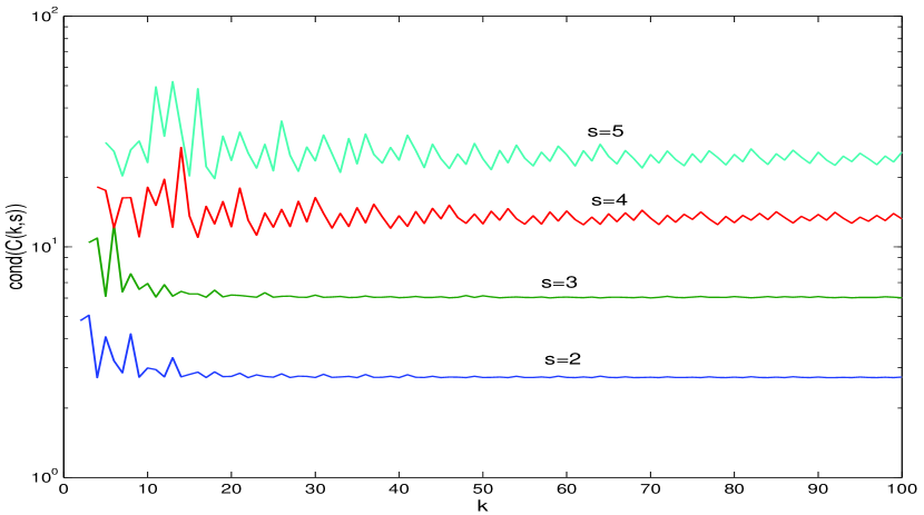
From the result of Theorem 2, it follows that the spectrum of doesn’t depend on the choice of the fundamental abscissae, within the nodes . On the contrary, its condition number does: the latter appears to be minimized when the fundamental abscissae are symmetrically distributed, and approximately evenly spaced, in the interval . As a practical “rule of thumb”, the following algorithm appears to be almost optimal:333We plan to investigate this aspect further, in a forthcoming paper.
-
1.
let the abscissae be chosen according to a Gauss-Legendre distribution of nodes;
-
2.
then, let us consider equidistributed nodes in , say ;
-
3.
select, as the fundamental abscissae, those nodes, among the , which are the closest ones to the ;
-
4.
define matrix in (37) accordingly.
Clearly, for the above algorithm to provide a unique solution (resulting in a symmetric choice of the fundamental abscissae), the difference has to be even which, however, can be easily accomplished.
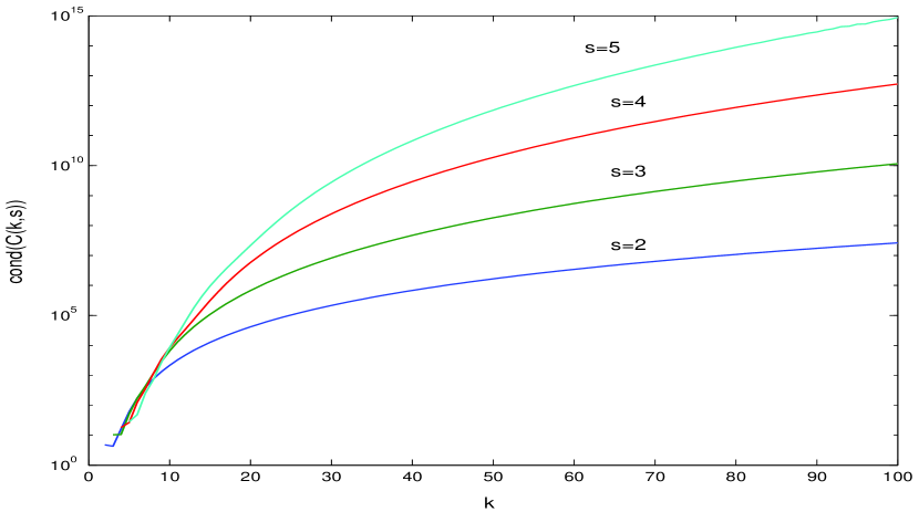
In order to give evidence of the effectiveness of the above algorithm, in Figure 2 we plot the condition number of matrix , for , and . As one can see, the condition number of turns out to be nicely bounded, for increasing values of , which makes the implementation (that we are going to analyze in the next section) effective also when finite precision arithmetic is used. For comparison, in Figure 2 there is the same plot, obtained by fixing the fundamental abscissae as the first ones.
5 Blended HBVMs
The solution of problem (38) is now cast into the framework of blended implicit methods B00 ; BM02 ; BM04 ; BM07 ; BM08 ; BMM06 ; BT2 ; M04 as below described. First of all, we observe that, since is nonsingular, we can recast problem (38) in the equivalent form
| (41) |
where is a free parameter to be chosen later. Let us now introduce the weight (matrix) function
| (42) |
and the blended formulation of the system to be solved,
| (43) | |||||
The latter system has still the same solution as the previous ones, since it is obtained as the blending, with weights and , of the two equivalent forms (38) and (41). For iteratively solving (43), we use the corresponding blended iteration, formally given by B00 ; BM02 ; BM04 ; BM07 ; BM08 ; BMM06 ; BT2 ; M04 :
| (44) |
Remark 7
A nonlinear variant of the iteration (44) can be obtained, by setting
and similarly defined, as:
| (45) |
Remark 8
We end this section by observing that the above iteration (44) depends on a free parameter . It will be chosen in order to optimize the convergence properties of the iteration, according to a linear analysis of convergence, which is sketched in the next section.
6 Linear analysis of convergence
The linear analysis of convergence for the iterations (44) is carried out by considering the usual scalar test equation (see, e.g., BM09 and the references therein),
By setting, as usual , the two equivalent formulations (38) and (41) become, respectively (omitting, for sake of brevity, the upper index ),
Moreover,
| (46) |
and the blended iteration (44) becomes
| (47) |
with
| (48) | |||||
Consequently, the iteration will be convergent if and only if the spectral radius, say , of the iteration matrix,
| (49) |
is less than 1. The set
is the region of convergence of the iteration. The iteration is said to be (see BM09 for details):
-
•
-convergent, if ;
-
•
-convergent, if it is -convergent and, moreover, , as .
For the iteration (47) one verifies that (see (46), (48), and (49))
| (50) |
which is the null matrix at and at . Consequently, the iteration will be -convergent (and, therefore, -convergent), provided that maximum amplification factor,
From (50) one has that 444Hereafter, will denote the spectrum of matrix .
By taking into account that
one then obtains that
For the Gauss-Legendre methods (and, then, for any matrix having the same spectrum), it can be shown that BM02 ; BMM06 the choice
| (51) |
minimizes , which turns out to be given by
| (52) |
In Table 1, we list the optimal value of the parameter , along with the corresponding maximum amplification factor , for various values of , which confirm that the iteration (47) is -convergent.
2 0.2887 0.1340 3 0.1967 0.2765 4 0.1475 0.3793 5 0.1173 0.4544 6 0.0971 0.5114 7 0.0827 0.5561 8 0.0718 0.5921 9 0.0635 0.6218 10 0.0568 0.6467
Remark 9
We then conclude that the blended iteration (44) turns out to be -convergent for HBVM methods, for all and .
7 Conclusions
In this paper, computational aspects related to the efficient implementation of HBVM methods with steps and degree () (in short, HBVM), have been recast in the framework of blended implicit methods. In more details, we have seen that the discrete problem generated by HBVM amounts to a nonlinear system of (block) dimension . Its efficient solution can be obtained by considering the blended formulation of the discrete problem, for which an efficient diagonal splitting can be easily defined. Consequently, to implement the nonlinear iteration, only one matrix having the same size as that of the continuous problem has to be factored. The free parameter, on which the blended iteration depends on, can be easily chosen, because of the isospectral property of HBVM, resulting in an -convergent iteration. Last, but not least, also the conditioning of the discrete problem depends only on , and it appears to tend to a (nicely) bounded limit, as grows. We plan, in the future, to implement HBVMs in blended formulation (in short, blended HBVMs), in a computational code for numerically solving Hamiltonian problems.
References
- (1) M. Abramovitz, I.A. Stegun. Handbook of Mathematical Functions. Dover, 1965.
- (2) L. Brugnano. Blended block BVMs (B3VMs): A family of economical implicit methods for ODEs. J. Comput. Appl.Math. 116 (2000) 41–62.
- (3) L. Brugnano, F. Iavernaro, T. Susca. Hamiltonian BVMs (HBVMs): implementation details and applications. “Proceedings of ICNAAM 2009”, AIP Conf. Proc. 1168 (2009) 723–726.
- (4) L. Brugnano, F. Iavernaro, D. Trigiante. Hamiltonian BVMs (HBVMs): a family of “drift-free” methods for integrating polynomial Hamiltonian systems. “Proceedings of ICNAAM 2009”, AIP Conf. Proc. 1168 (2009) 715–718.
- (5) L. Brugnano, F. Iavernaro, D. Trigiante. Analisys of Hamiltonian Boundary Value Methods (HBVMs): a class of energy-preserving Runge-Kutta methods for the numerical solution of polynomial Hamiltonian dynamical systems. BIT (2009), submitted. (arXiv:0909.5659)
- (6) L. Brugnano, F. Iavernaro, D. Trigiante. Hamiltonian Boundary Value Methods (Energy Preserving Discrete Line Integral Methods). Jour. of Numer. Anal., Industr. and Appl. Math. (2009) submitted. (arXiv:0910.3621)
- (7) L. Brugnano, C. Magherini. Blended implementation of block implicit methods for ODEs. Appl. Numer. Math. 42 (2002) 29–45.
- (8) L. Brugnano, C. Magherini. The BiM code for the numerical solution of ODEs. J. Comput. Appl. Math. 164–165 (2004) 145–158.
- (9) L. Brugnano, C. Magherini. Blended implicit methods for solving ODE and DAE problems, and their extension for second order problems. J. Comput. Appl. Math. 205 (2007) 777–790.
- (10) L. Brugnano, C. Magherini. Blended General Linear Methods based on Generalized BDF. AIP Conf. Proc. 1048 (2008) 871–874.
- (11) L. Brugnano, C. Magherini. Recent Advances in Linear Analysis of Convergence for Splittings for Solving ODE problems. Appl. Numer. Math. 59 (2009) 542–557.
- (12) L. Brugnano, C. Magherini. Blended General Linear Methods based on Boundary Value Methods in the GBDF family. Journal of Numerical Analysis, Industrial and Applied Mathematics 4, 1-2 (2009) 23–40.
- (13) L Brugnano, C. Magherini, F. Mugnai. Blended implicit methods for the numerical solution of DAE problems. J. Comput. Appl. Math. 189 (2006) 34–50.
- (14) L. Brugnano, D. Trigiante. Solving Differential Problems by Multistep Initial and Boundary Value Methods. Gordon and Breach, Amsterdam, 1998.
- (15) L. Brugnano, D. Trigiante. Block implicit methods for ODEs, in: D. Trigiante (Ed.), Recent Trends in Numerical Analysis. Nova Science Publ. Inc., New York, 2001, pp. 81–105.
- (16) E. Hairer, C. Lubich, G. Wanner. Geometric Numerical Integration. Structure-Preserving Algorithms for Ordinary Differential Equations, 2nd ed., Springer, Berlin, 2006.
- (17) E. Hairer, G. Wanner. Solving Ordinary Differential Equations II, 2nd ed., Springer, Berlin, 1996.
- (18) F. Iavernaro, B. Pace. -Stage Trapezoidal Methods for the Conservation of Hamiltonian Functions of Polynomial Type. AIP Conf. Proc. 936 (2007) 603–606.
- (19) F. Iavernaro, B. Pace. Conservative Block-Boundary Value Methods for the Solution of Polynomial Hamiltonian Systems. AIP Conf. Proc. 1048 (2008) 888–891.
- (20) F. Iavernaro, D. Trigiante. Discrete conservative vector fields induced by the trapezoidal method. J. Numer. Anal. Ind. Appl. Math. 1 (2006) 113–130.
- (21) F. Iavernaro, D. Trigiante. State-dependent symplecticity and area preserving numerical methods. J. Comput. Appl. Math. 205 no. 2 (2007) 814–825.
- (22) F. Iavernaro, D. Trigiante. High-order symmetric schemes for the energy conservation of polynomial Hamiltonian problems. J. Numer. Anal. Ind. Appl. Math. 4,1-2 (2009) 87–101.
- (23) C. Magherini. Numerical Solution of Stiff ODE-IVPs via Blended Implicit Methods: Theory and Numerics. PhD thesis, Dipartimento di Matematica “U. Dini”, Università degli Studi di Firenze, September 2004 (Available at the url BIMcode ).
- (24) Codes BiM/BiMD Homepage: http://www.math.unifi.it/~brugnano/BiM/index.html
- (25) Test Set for IVP Solvers (release 2.4): http://pitagora.dm.uniba.it/~testset/