Cross-correlation of the HI 21-cm Signal and Lyman-$\alpha$ Forest: A Probe Of Cosmology

Abstract

Separating the cosmological redshifted 21-cm signal from foregrounds is a major challenge. We present the cross-correlation of the redshifted 21-cm emission from neutral hydrogen (HI) in the post-reionization era with the Ly-$\alpha$ forest as a new probe of the large scale matter distribution in the redshift range $z=2$ to $3$ without the problem of foreground contamination. Though the 21-cm and the Ly-$\alpha$ forest signals originate from different astrophysical systems, they are both expected to trace the underlying dark matter distribution on large scales. The multi-frequency angular cross-correlation power spectrum estimator is found to be unaffected by the discrete quasar sampling, which only affects the noise in the estimate.

We consider a hypothetical redshifted 21-cm observation in a single field of view $1.3^{\circ}$ (FWHM) centered at $z=2.2$ where the binned 21-cm angular power spectrum can be measured at an SNR of $3\sigma$ or better across the range $500\leq\ell\leq 4000$. Keeping the parameters of the 21-cm observation fixed, we have estimated the SNR for the cross-correlation signal varying the quasar angular number density $n$ of the Ly-$\alpha$ forest survey. Assuming that the spectra have SNR $\sim 5$ in pixels of length $44\,{\rm km/s}$, we find that a $5\sigma$ detection of the cross-correlation signal is possible at $600\leq\ell\leq 2000$ with $n=4\ {\rm deg}^{-2}$. This value of $n$ is well within the reach of upcoming Ly-$\alpha$ forest surveys. The cross-correlation signal will be a new, independent probe of the astrophysics of the diffuse IGM, the growth of structure and the expansion history of the Universe.

1 Introduction.

Observations of the redshifted 21-cm radiation from neutral hydrogen (HI) provides an unique opportunity for probing the cosmological matter distribution over a wide range of redshifts $(0\leq z\leq 200)$ and there currently is considerable effort underway towards detecting this (Furlanetto et al., 2006; Lewis & Challinor, 2007; Morales & Wyithe, 2009). Foregrounds from other astronomical sources which are several orders of magnitude larger, however, pose a severe challenge for detecting this signal (Santos et al., 2005; McQuinn et al., 2006; Ali et al., 2008). The 21-cm emission from the post-reionization era ($z<6$) is of particular interest (Saini et al., 2001; Bharadwaj & Sethi, 2001; Bharadwaj et al., 2001; Wyithe & Loeb, 2007) because the foregrounds are relatively smaller and the HI is expected to trace the underlying dark matter with a possible bias. These observations hold the possibility of measuring both the matter power spectrum and the cosmological parameters (Wyithe et al., 2007; Chang et al., 2008; Bharadwaj et al., 2009).

Interestingly, diffused HI in the intervening intergalactic medium in the same $z$ range, produces a large number of absorption lines (Lyman-$\alpha$ forest) in the spectra of distant quasars (QSO). These low neutral density absorption lines are caused due to small baryonic fluctuations in the IGM and has the potential to probe the matter distribution and baryonic structure formation to very small scales. Here the the Ly-$\alpha$ forest, whose fluctuations is believed to trace the underlying dark matter, is of special interest. The Ly-$\alpha$ forest is known to be a valuable cosmological probe (Mandelbaum et al., 2003). This has found a variety of applications which include determining the matter power spectrum (Croft et al., 1998, 1999; Lesgourgues et al., 2007), cosmological parameter estimation (Seljak et al., 2006; McDonald & Eisenstein, 2007; Gratton et al., 2008), constraining the clustering properties of dark matter on small scales (Viel et al., 2008) and probing the reionization history (Hui & Gnedin, 1997; Gallerani et al., 2006; Cen et al., 2009).

Though the 21-cm emission and the Ly-$\alpha$ forest both originate from HI at the same $z$, these two signals originate from two different kinds of astrophysical systems. The Ly-$\alpha$ forest originates from small HI fluctuations present in the primarily ionized IGM; the 21-cm emission from these regions is completely negligible. On the other hand, the bulk of the 21-cm signal originate from Damped Ly-$\alpha$ Absorbers (DLAs) which contain most of the neutral hydrogen at these epochs (Lanzetta et al., 1995; Storrie-Lombardi et al., 1996; P’eroux et al., 2003). It is however reasonable to assume that on large scales both these traces the same underlying dark matter, and hence we may expect them to be correlated.

In this paper, we propose a novel probe of the large scale matter distribution using the cross-correlation of the 21-cm brightness temperature and the Ly-$\alpha$ forest transmitted flux. The cross-correlation signal holds the potential of independently unveiling the same astrophysical and cosmological information as the individual auto-correlations, with the added advantage that the problems of foregrounds and systematics are expected to be much less severe for the cross-correlation. We note earlier studies that consider the possibility of cross-correlating the Ly-$\alpha$ forest with the CMBR (Croft et al., 2006) and weak lensing Vallinotto et al. (2009), and cross-correlating the post-reionization 21-cm signal with the CMBR (Guha Sarkar et al., 2009) and weak lensing (Guha Sarkar, 2010). The cosmological 21-cm signal has recently been detected through cross-correlations with the 6dfGRS (Pen et al., 2009) and the DEEP2 optical galaxy redshift survey (Chang et al., 2010).

2 The Cross-correlation Angular power Spectrum.

The fluctuations in the transmitted flux ${{\mathcal{F}}}({\bf{\hat{n}}},z)$ along a line of sight ${\bf{\hat{n}}}$ in the Ly-$\alpha$ forest may be quantified using $\delta_{{\mathcal{F}}}({\bf{\hat{n}}},z)={{\mathcal{F}}}({\bf{\hat{n}}},z)/\bar{{\mathcal{F}}}-1$. At the large scales of interest here it is reasonable to adopt the fluctuating Gunn-Peterson approximation (Gunn & Peterson, 1965; Bi & Davidsen, 1997; Croft et al., 1998, 1999) which relates the flux and the matter density contrast as ${{\mathcal{F}}}=\exp[-A(1+\delta)^{\kappa}]$ where $A$ and $\kappa$ are two redshift dependent functions. The function $A$ is of order unity and depends on the mean flux level, IGM temperature, photo-ionization rate and cosmological parameters, while $\kappa$ depends on the IGM temperature density relation (McDonald et al., 2001; Choudhury et al., 2001). For a preliminary analytic estimate of the cross-correlation signal, we assume that $\delta_{{\mathcal{F}}}$ has been smoothed whereby it is adequate to retain only the linear term $\delta_{{\mathcal{F}}}\propto\,\delta$ (Croft et al., 1998; Bi & Davidsen, 1997; Viel et al., 2002; Slosar et al., 2009) The higher order terms, which have been dropped to keep the analytic calculations tractable, will, in principle, contribute to the cross-correlation. We plan to address this in future studies using simulations.

In the redshift range of our interest ($z<3.5$) the fluctuation in the redshifted 21-cm brightness temperature $\delta_{T}({\bf{\hat{n}}},z)$ traces the underlying dark matter distribution with a possible scale dependent bias function $b_{T}(k,z)$. The bias is expected to be scale dependent below the Jeans length-scale (Fang et al., 1993), and fluctuations in the ionizing background (Wyithe & Loeb, 2007, 2009) also give rise to a scale dependent bias. Further, this bias is found to grow monotonically with $z$ for $1<z<4$ (Marin et al., 2009). However, the simulations of (Bagla et al., 2009), and also (Wyithe & Loeb, 2009) indicate that a constant, scale independent bias is adequate at the large scales of our interest ( $\ell<6000$ at $z\sim 2.2$). We have used the constant value $b_{T}=2$ in our analysis.

With these assumptions and incorporating redshift space distortions we may express both $\delta_{{\mathcal{F}}}$ and $\delta_{T}$ as

$$\delta_{\alpha}({\bf{\hat{n}}},z)=C_{\alpha}\int\ \frac{d^{3}{\bf{k}}}{(2\pi)^{3}}\ e^{i{\bf{k}}.{\bf{\hat{n}}}r}[1+\beta_{\alpha}\mu^{2}]\Delta({\bf{k}})\,.$$ (1)

where $\alpha={{\mathcal{F}}},T$ refers to the Ly-$\alpha$ flux and 21-cm brightness temperature respectively, $r$ is the comoving distance, $\Delta({\bf{k}})$ is the dark matter density contrast in Fourier space and $\mu={\bf\hat{k}\cdot\hat{n}}$. We adopt $C_{{\mathcal{F}}}=-0.13$ and $\beta_{{\mathcal{F}}}=1.58$ from numerical simulations of the Ly-$\alpha$ forest (McDonald, 2003).

For the 21-cm we use $C_{T}=\bar{T}\,\bar{x}_{\rm HI}\,b$ and $\beta_{T}=f/b$ (Bharadwaj & Ali, 2004, 2005), where

$$\bar{T}(z)=4.0\rm mK\,(1+z)^{2}\ \left(\frac{\Omega_{b0}h^{2}}{0.02}\right)\,\left(\frac{0.7}{h}\right)\,\left(\frac{H_{0}}{H(z)}\right),$$ (2)

$\bar{x}_{\rm HI}$ is the mean neutral hydrogen fraction, $f$ is the linear growth parameter of density fluctuations and $b_{T}$ is the bias. At redshifts $0\leq z\leq 3.5$ we have $\Omega_{gas}\sim 10^{-3}$ (Lanzetta et al., 1995; Storrie-Lombardi et al., 1996) which implies that $\bar{x}_{\rm HI}=50\,\Omega_{gas}h^{2}\,(0.02/\Omega_{b}h^{2})=2.45\times 10^{-2}$ used here. As mentioned earlier, numerical simulations (Khandai et al., 2009) suggest that $b\approx 2$ which we adopt here.

Consider next a field of view that is sufficiently small such that it may be treated as being flat. We may then express the unit vector along the line of sight as ${\bf{\hat{n}}}=\hat{\bf{m}}+\vec{\theta}$, where $\hat{\bf{m}}$ is the line of sight to the centre of the field of view and $\vec{\theta}$ is a two-dimensional ($2D$) vector on the sky ($\theta<<1$). In this flat sky approximation it is convenient to decompose $\delta_{{\mathcal{F}}}(\vec{\theta},z)$ and $\delta_{T}(\vec{\theta},z)$ into Fourier modes where we use ${\bf U}$ as the variable conjugate to $\vec{\theta}$. Following Datta et al. (2007), we define the multi-frequency angular power spectrum (MAPS) as

$$P_{a}({\bf U},\Delta z)=\frac{1}{\pi r^{2}}\int_{0}^{\infty}dk_{\parallel}\ \cos(k_{\parallel}\Delta r)\ F_{a}(\mu)\ P(k)\,.$$ (3)

Here $a=T$ refers to the HI 21-cm brightness temperature fluctuation power spectrum of $\delta_{T}(\vec{\theta},z)$ and $\delta_{T}(\vec{\theta},z+\Delta z)$ at two slightly different redshifts $z$ and $z+\Delta z$. Similarly, $a={\mathcal{F}}$ and $a=c$ respectively refer to the Ly-$\alpha$ forest and $\delta_{T}-\delta_{{\mathcal{F}}}$ cross-correlation power spectra. In eq. (3), $\Delta r$ is the radial comoving separation corresponding to $\Delta z$, $P(k)$ is the dark matter power spectrum, $k=\sqrt{k_{\parallel}^{2}+(\frac{2\pi U}{r})^{2}}$ and $\mu=k_{\parallel}/k$. The function $F_{a}(\mu)$ takes values $A^{2}(\mu)$ , $B^{2}(\mu)$ and $A(\mu)\ B(\mu)$ corresponding to $a=T$, ${{\mathcal{F}}}$ and $c$ respectively. Here $A(\mu)=C_{T}[1+\beta_{T}\mu^{2}]$ and $B(\mu)=C_{{\mathcal{F}}}[1+\beta_{{\mathcal{F}}}\mu^{2}]$. We note that the MAPS $P_{a}({\bf U},\Delta z)$, which is directly related to observable quantities, contains the entire information of the three dimensional (3D) power spectrum through its $U$ and $\Delta z$ dependence.

Given a field of view, it will be possible to probe $\delta_{{\mathcal{F}}}$ only along a few, discrete lines of sight corresponding to the angular positions of the bright quasars. We incorporate this through a sampling function which is a sum of Dirac delta functions $\rho(\vec{\theta})=N^{-1}\ \sum_{n}\delta_{D}^{2}(\vec{\theta}-\vec{\theta}_{n})$ where $\vec{\theta}_{n}$ refers to the angular positions of the quasars and the summation extends up to $N$, the number of quasars in the field of view. Taking into account the discrete sampling, the observed Ly-$\alpha$ forest flux fluctuation may be written as $\delta_{{{\mathcal{F}}}o}(\vec{\theta})=\rho(\vec{\theta})\ \delta_{{\mathcal{F}}}(\vec{\theta})$. The aim here being to detect the cross-correlation power spectrum, we define the estimator

$$\hat{E}({\bf U},\Delta z)=\frac{1}{2}\left[\tilde{\delta}_{{{\mathcal{F}}}o}({\bf U},z)\ \tilde{\delta}_{T}^{*}({\bf U},z+\Delta z)\right]$$

$$+\frac{1}{2}\left[\tilde{\delta}_{{{\mathcal{F}}}o}^{*}({\bf U},z)\ \tilde{\delta}_{T}({\bf U},z+\Delta z)\right].$$ (4)

where tilde denotes the 2D Fourier transform. While it has been assumed that the Ly-$\alpha$ forest and the HI 21-cm brightness temperature both traces the same underlying dark matter distribution, with possibly different bias parameters, the quasars are assumed to be at a higher redshift and hence uncorrelated with either ${\mathcal{F}}$ or $T$. Using this, we have the expectation value and variance of the estimator to be

$$\langle\hat{E}({\bf U},\Delta z)\rangle=P_{c}({\bf U},\Delta z)$$ (5)

and

$$\langle(\Delta\hat{E})^{2}\rangle=\frac{1}{2}P_{c}^{2}({\bf U},\Delta z)+\frac{1}{2}\left[P_{T}({\bf U},0)+N_{T}\right]$$

$$\times\left[\frac{1}{n}\int d^{2}{\bf U}^{\prime}P_{{\mathcal{F}}}({\bf U}^{\prime},0)+P_{{\mathcal{F}}}({\bf U},0)+N_{{\mathcal{F}}}\right]$$ (6)

where $N_{T}$ and $N_{\mathcal{F}}$ are the respective noise power spectra for $T$ and ${\mathcal{F}}$, it being assumed that the two noises are uncorrelated. The quasars, with angular number density $n$, have been assumed to be randomly distributed and their clustering has been ignored. We assume that the variance $\sigma^{2}_{{{\mathcal{F}}}N}$ of the pixel noise contribution to $\delta_{{\mathcal{F}}}$ is the same across all the quasar spectra whereby we have $N_{\mathcal{F}}=\sigma^{2}_{{{\mathcal{F}}}N}/n$ for its noise power spectrum. The integral in eq. (6) can be simplified using eq. (3) to calculate $P_{{\mathcal{F}}}({\bf U}^{\prime},0)$ whereby

$$\int d^{2}{\bf U}^{\prime}\ P_{{\mathcal{F}}}({\bf U}^{\prime},0)\ =\ \int\frac{d^{3}{\bf k}}{(2\pi)^{3}}\ C_{{\mathcal{F}}}^{2}[1+\beta_{{\mathcal{F}}}\mu^{2}]^{2}P(k)=\sigma_{{\mathcal{F}}L}^{2}$$ (7)

where ${\bf k}\equiv(2\pi{\bf U}/r,k_{\parallel})$ and $\sigma^{2}_{{\mathcal{F}}L}$ is the variance of the fluctuations in the smoothed $\delta_{{\mathcal{F}}}$ arising from the large scale matter fluctuations and peculiar velocities. We have the total variance of $\delta_{{\mathcal{F}}}$ as $\sigma^{2}_{{\mathcal{F}}}=\sigma^{2}_{{\mathcal{F}}N}+\sigma^{2}_{{\mathcal{F}}L}$ whereby the variance of the cross-correlation estimator is

$$\langle(\Delta\hat{E})^{2}\rangle=\frac{1}{2}\left\{P_{c}^{2}({\bf U},\Delta z)+\left[P_{T}({\bf U},0)+N_{T}\right]\right.$$

$$\left.\left[P_{{\mathcal{F}}}({\bf U},0)+\frac{\sigma^{2}_{{\mathcal{F}}}}{n}\right]\right\}$$ (8)

The cross-correlation signal being statistically isotropic on the sky, we may combine estimates of the power spectrum over different directions of ${\bf U}$ to reduce the uncertainty (or variance) in the estimated cross-correlation signal. Binning in $U$ and combining estimates at different redshift values within the observational bandwidth lead to a further reduction of the uncertainty. Finally, incorporating the possibility of observations in several independent fields of view, we use $N_{E}$ to denote the total number of independent estimates that are combined. The uncertainty or noise in the resulting combined estimate of $P_{c}(U,\Delta z)$ is $\sigma^{2}\ =\ \langle(\Delta\hat{E})^{2}\rangle/{N_{E}}\,$. It is convenient to express our results in terms of the angular multipole $\ell=\ 2\pi U$. We then have $N_{E}=(\ell+\frac{1}{2})\,\Delta\ell\,(B/\Delta\nu)\,f\,N_{F}$ where $\Delta\ell$ is the width of the $\ell$ bin, $B$ the frequency bandwidth of the 21-cm observation, $\Delta\nu$ the frequency interval beyond which we have an independent estimate of the signal, $f$ the fraction of the sky covered by a single field of view and $N_{F}$ the number of independent fields of view that are observed.

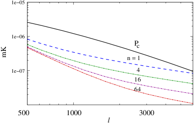
Figure 1: The magnitude of the cross-correlation angular power spectrum (topmost curve) and $1\sigma$ errors (lower curves) for $z=2.2$. Note that $\delta_{{\mathcal{F}}}$ and $\delta_{T}$ are anti-correlated.

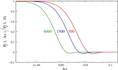
Figure 2: The decorrelation of $P_{c}(\ell,\Delta z)$ with increasing $\Delta z$ for the representative $\ell$ values shown in the figure.

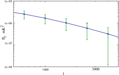
Figure 3: The HI 21-cm angular power spectrum for $z=2.2$ with $3\sigma$ error bars

3 Detectability.

We next estimate the survey parameters that will be required to detect the cross-correlation signal. It is, in principle, possible to vary the parameters of both the redshifted 21-cm survey and the Ly-$\alpha$ survey. To keep the analysis simple we restrict our attention to a situation where the parameters of the redshifted 21-cm survey are fixed, and vary the parameters of only the Ly-$\alpha$ survey.

The quasar distribution is known to peak between $z=2$ and $3$. For any particular quasar, it is possible to reliably estimate $\delta_{{\mathcal{F}}}$ in a small redshift range close to the quasar’s redshift. The region very close to the quasar is excluded due to the quasar’s Stromgren sphere, and large redshift separations are excluded to avoid Ly-$\beta$ contamination. Based on this we have only considered quasars in the $z$ range $2.2-3.0$ for our estimates, and we have chosen a region centered at $z=2.2$ for our estimates.

The predicted HI- ${\mathcal{F}}$ cross correlation angular power spectrum is shown (Figures 1 and 2) assuming cosmological parameters from WMAP $5$ results (Komatsu et al., 2009). The $\ell$ dependence closely follows that of the HI angular power spectrum (Figure 3). The signals at two different redshifts $z$ and $z+\Delta z$, we find, decorrelate rapidly with increasing $\Delta z$, the decline being faster at larger $\ell$ values.

The currently functioning GMRT (Swarup et al., 1991) can, in principle be used to probe the redshifted HI 21-cm signal all the way from $z\sim 0$ to $z\sim 8$ (Bharadwaj & Ali, 2005). The GMRT, at present, has neither the exact frequency band nor the desired sensitivity for the proposed observation. In principle it would not be very difficult, in future, to cover the required frequency and increase the number of antennas to increase the sensitivity. For the present analysis we consider a hypothetical array, possibly an extended version of the GMRT or some other future radio telescope with 60 antennas similar to the GMRT, distributed randomly over a 1 km $\times$ 1 km square. Note that this is roughly $4$ times the number of antennas currently available in the GMRT central square, and henceforth we refer to this as the extended GMRT (EGMRT). Each antenna is $45\,{\rm m}$ in diameter, with a field of view $1.3^{\circ}$ (FWHM), total system temperature $100\,{\rm K}$ and antenna gain $0.33\,{\rm K/Jy}$. We assume that the observations are carried out over a frequency band of $32\,{\rm MHz}$ centered at $430\,{\rm MHz}$ using channels of width $62.5\,{\rm kHz}$ each. The frequency separation $\Delta\nu$ over which the 21-cm signal remains correlated roughly scales as $\Delta\nu=1\,{\rm MHz}\,(\ell/100)^{-0.7}$ (Bharadwaj & Pandey, 2003). We assume that the signal is averaged over frequency bins of this width to increase the SNR. Considering $1,000$ hrs of observation in a single field of view, a $3\ \sigma$ (or better) measurement of the HI 21-cm power spectrum will be possible at $\ell\leq 4000$ (Figure 3). Note that the error is dominated by the system noise, the cosmic variance being considerably smaller. This justifies why we have considered observations in a single field of view instead of distributing the $1000\,{\rm hr}$ observation over different fields.

Considering next the Ly-$\alpha$ forest surveys, we note that these typically cover a much larger angular region and redshift interval compared to the 21-cm observation that we have considered. For example, the SDSS Data Release 3 (Schneider et al., 2005), whose data is currently available, covers $4,188\ {\rm deg}^{2}$ of the sky. The number density of quasars in the redshift range $z=2.2-3.0$ is $n=1.0\ {\rm deg}^{-2}$ for this survey. The cross-correlation is restricted to the angular extent of the 21-cm observation and the redshift interval $\Delta z=0.24$ centered at $z=2.2$ which corresponds to a bandwidth of $32\,{\rm MHz}$ centered at $430\,{\rm MHz}$. The channel width $62.5\,{\rm kHz}$ of the 21-cm observations corresponds to $\Delta z=4.7\times 10^{-4}$ or equivalently $v_{\parallel}=44\,{\rm km/s}$.

The analysis of fluctuations in the Lyman-$\alpha$ forest (D’Odorico et al., 2006; Coppolani et al., 2006) show that the variance has a value $\sigma^{2}_{{\mathcal{F}}L}\approx 0.02$ for $\delta_{{\mathcal{F}}}$ smoothed over $\sim 50\,{\rm km/s}$ along the line of sight. This smoothing is comparable to the channel width of the 21-cm observations, and for simplicity we assume that Ly-$\alpha$ pixel length is exactly the same as the 21-cm channel width. Note that this is smaller than the typical $\Delta z$ value where the signal decorrelates (Figure 2). For the pixel noise contribution, we assume that $S/N=5$ for every pixel of the spectra used to estimate the cross-correlation. This gives $\sigma^{2}_{{\mathcal{F}}N}=0.04$, whereby $\sigma^{2}_{{\mathcal{F}}}=0.06$ for pixels of length $44\,{\rm km/s}$ or $62.5\,{\rm kHz}$. As noted earlier, it is advantageous to average the signal over an interval $\Delta\nu=1\,{\rm MHz}\,(\ell/100)^{-0.7}\geq 62.5\,{\rm kHz}$ before correlating. The value of $\sigma^{2}_{{\mathcal{F}}}$ will come down due to this averaging. Assuming that the pixel noise in different pixels is uncorrelated, we have $\sigma^{2}_{{\mathcal{F}}N}=0.04\ (62.5\,{\rm kHz}/\Delta\nu)$. Analysis of the line of sight correlation function of $\delta_{{\mathcal{F}}}$ indicate that we may expect $\sigma^{2}_{{\mathcal{F}}L}$ to scale faster than $(\Delta\nu)^{-1}$. For the purpose of this paper we assume that both $\sigma^{2}_{{\mathcal{F}}L}$ and $\sigma^{2}_{{\mathcal{F}}N}$ have the same scaling whereby $\sigma^{2}_{{\mathcal{F}}}=0.06\ (62.5\,{\rm kHz}/\Delta\nu)$. which we use in eq. (8) for our noise estimates. The error introduced by the last assumption, will at worst, cause the noise for the cross-correlation signal to be over-estimated.

We present noise estimates (Figure 1) considering quasar angular number densities $n=1,4,\ 16$ and $64\ {\rm deg}^{-2}$. While our intention is primarily to estimate the quasar number density that will be required to detect the cross-correlation signal, we note that the $n$ values chosen are viable with existing or future surveys. The currently available SDSS (Schneider et al., 2005) has $n\sim 1{\rm deg}^{-2}$ and the upcoming BOSS(McDonald et al., 2005) is expected to have $n\sim 16{\rm deg}^{-2}$, while the proposed future BIGBOSS (Schlegel et al., 2009) is anticipated to reach $n>64{\rm deg}^{-2}$. We find that a $3\sigma$ and $5\sigma$ detection will be possible at $\ell\leq 2000$ for $n=1$ and $4\ {\rm deg}^{-2}$ respectively. A $5\sigma$ (or better) detection will be possible over the entire $\ell$ range for $n=16$ and $64\,{\rm deg}^{-2}$. There is a further reduction of noise by a factor $N_{F}^{-1/2}$ if the same observation is repeated in multiple fields of view.

Unlike the $\delta_{{\mathcal{F}}}$ auto-correlation power spectrum which is Poisson noise dominated, the cross-correlation signal itself is not affected by the discrete quasar sampling. However its variance is very sensitive to this, and a dense quasar sampling will allow the cross-correlation to be measured at a high level of precision.

The discussion so far has completely bypassed several observational difficulties which pose a severe challenge. Considering first the Ly-$\alpha$ forest, errors in continuum fitting and subtraction would result in an additive error in the estimated $\delta_{{\mathcal{F}}}$ which will inhibit recovery of the underlying power spectrum at large scales. Croft et al. (2002) and McDonald et al. (2006) have studied this issue extensively and have proposed several techniques to mitigate the contribution from such errors. While an additive error in $\delta_{{\mathcal{F}}}$ could have severe repercussions for the large-scale power spectrum estimated from the auto-correlation of $\delta_{{\mathcal{F}}}$ (Kim et al., 2004), we do not expect these errors to be correlated with the 21-cm data. An additive error in $\delta_{{\mathcal{F}}}$ will manifest itself as an extra contribution to the noise for the cross-correlation power spectrum (eq. 8) which, in turn may degrade the SNR and hence affect the detectability of the cross-correlation signal.

The redshifted 21-cm signal is buried under foregrounds which are several orders of magnitude larger (Shaver et al., 1999; Di Matteo et al., 2002; Santos et al., 2005; Wang & Hu, 2006; Ali et al., 2008; Bernardi et al., 2009; Pen et al., 2009; Ghosh et al., 2010). Extragalactic point sources and the diffuse synchrotron radiation from our own Galaxy are the two most dominant foreground components. The free-free emissions from our Galaxy and external galaxies make much smaller contributions (Shaver et al., 1999), though each of these is individually larger than the HI signal. Several different techniques have been proposed for separating the 21-cm signal from the foregrounds. All of these depend on the fact that the foregrounds are expected to have a continuum frequency spectrum, and their contribution at two different frequencies separated by $\Delta\nu$ is expected to be correlated well beyond $\Delta\nu\sim 5\,{\rm MHz}$ . The 21-cm signal, however, is predicted to decorrelate within $\Delta\nu\sim 1\,{\rm MHz}$ for angular scales of our interest (Bharadwaj & Sethi, 2001). A possible technique for foreground removal is to subtract out any smooth frequency dependent component either from the image cube (Jelić et al., 2008; Bowman et al., 2009; Liu et al., 2009) or from the gridded visibilities (Liu et al., 2009). Another possible approach is to first estimate the multi-frequency angular power spectrum of the radio-interferometric data and then subtract out any component that remains correlated over large frequency separations (Ali et al., 2008; Ghosh et al., 2010).

The foregrounds of the redshifted 21-cm signal are expected to be uncorrelated with the Ly-$\alpha$ forest $\delta_{{\mathcal{F}}}$ and also any errors arising in it from continuum subtraction. We do not expect the foregrounds to contribute to the estimated cross-correlation signal, and we anticipate that the problem of foreground removal will be considerably less severe as compared to the auto-correlation. Errors in foreground subtraction will manifest as an extra source of noise for the cross-correlation signal. The fact that the 21-cm $\delta_{T}$ and the Ly-$\alpha$ $\delta_{{\mathcal{F}}}$ at two different redshifts separated by $\Delta z$ decorrelate rapidly as $\Delta z$ is increased (Figure 2) should help in identifying any foreground contamination.

Errors in calibrating the radio observations is another possible source of uncertainty in the 21-cm signal. This will lead to errors in the overall amplitude of the cross-correlation signal, or equivalently contribute to uncertainties in estimates of the quantity $C_{{\mathcal{F}}}C_{T}$ defined in Section 2.

In conclusion, we propose the 21-cm and Ly-$\alpha$ forest cross-correlation signal as a tool to measure the large-scale matter distribution. The problem of foreground removal is expected to be considerable less severe for the cross-correlation than for the 21-cm auto correlation signal.The cross-correlation signal will probe a variety of issues like the astrophysics of the diffuse IGM, the growth of large-scale structures and the expansion history of the Universe.

References

- Ali et al. (2008) Ali S. S., Bharadwaj S., Chengalur J. N., 2008, MNRAS, 385, 2166
- Bagla et al. (2009) Bagla J. S., Khandai N., Datta, K. K. 2009, ArXiv e-prints
- Bernardi et al. (2009) Bernardi G., de Bruyn A. G., Brentjens M. A., Ciardi B., 2009, Astron. Astrophys., 500, 965
- Bharadwaj & Ali (2004) Bharadwaj S., Ali S. S., 2004, MNRAS, 352, 142
- Bharadwaj & Ali (2005) Bharadwaj S., Ali S. S., 2005, MNRAS, 356, 1519
- Bharadwaj et al. (2001) Bharadwaj S., Nath B. B., Sethi S. K., 2001, Journal of Astrophysics and Astronomy, 22, 21
- Bharadwaj & Pandey (2003) Bharadwaj S., Pandey S. K., 2003, Journal of Astrophysics and Astronomy, 24, 23
- Bharadwaj & Sethi (2001) Bharadwaj S., Sethi S. K., 2001, Journal of Astrophysics and Astronomy, 22, 293
- Bharadwaj et al. (2009) Bharadwaj S., Sethi S. K., Saini T. D., 2009, PRD, 79, 083538
- Bi & Davidsen (1997) Bi H., Davidsen A. F., 1997, ApJ, 479, 523
- Bowman et al. (2009) Bowman J. D., Morales M. F., Hewitt J. N., 2009, ApJ, 695, 183
- Cen et al. (2009) Cen R., McDonald P., Trac H., Loeb A., 2009, ApJL, 706, L164
- Chang et al. (2010) Chang T., Pen U., Bandura K., Peterson J. B., 2010, Nature, 466, 463
- Chang et al. (2008) Chang T., Pen U., Peterson J. B., McDonald P., 2008, Physical Review Letters, 100, 091303
- Choudhury et al. (2001) Choudhury T. R., Padmanabhan T., Srianand R., 2001, MNRAS, 322, 561
- Coppolani et al. (2006) Coppolani F., Petitjean P., Stoehr F., Rollinde E., Pichon C., Colombi S., Haehnelt M. G., Carswell B., Teyssier R., 2006, MNRAS, 370, 1804
- Croft et al. (2006) Croft R. A. C., Banday A. J., Hernquist L., 2006, MNRAS, 369, 1090
- Croft et al. (2002) Croft R. A. C., Weinberg D. H., Bolte M., Burles S., Hernquist L., Katz N., Kirkman D., Tytler D., 2002, ApJ, 581, 20
- Croft et al. (1998) Croft R. A. C., Weinberg D. H., Katz N., Hernquist L., 1998, ApJ, 495, 44
- Croft et al. (1999) Croft R. A. C., Weinberg D. H., Pettini M., Hernquist L., Katz N., 1999, ApJ, 520, 1
- Datta et al. (2007) Datta K. K., Choudhury T. R., Bharadwaj S., 2007, MNRAS, 378, 119
- Di Matteo et al. (2002) Di Matteo T., Perna R., Abel T., Rees M. J., 2002, ApJ, 564, 576
- D’Odorico et al. (2006) D’Odorico V., Viel M., Saitta F., Cristiani S., Bianchi S., Boyle B., Lopez S., Maza J., Outram P., 2006, MNRAS, 372, 1333
- Fang et al. (1993) Fang L., Bi H., Xiang S., Boerner G., 1993, ApJ, 413, 477
- Furlanetto et al. (2006) Furlanetto S. R., Oh S. P., Briggs F. H., 2006, Physics Report, 433, 181
- Gallerani et al. (2006) Gallerani S., Choudhury T. R., Ferrara A., 2006, MNRAS, 370, 1401
- Ghosh et al. (2010) Ghosh A., Bharadwaj S., Ali S. S., Chengalur J., 2010, Submitted to MNRAS
- Gratton et al. (2008) Gratton S., Lewis A., Efstathiou G., 2008, PRD, 77, 083507
- Guha Sarkar (2010) Guha Sarkar T., 2010, Journal of Cosmology and Astro-Particle Physics, 2, 2
- Guha Sarkar et al. (2009) Guha Sarkar T., Datta K. K., Bharadwaj S., 2009, Journal of Cosmology and Astro-Particle Physics, 8, 19
- Gunn & Peterson (1965) Gunn J. E., Peterson B. A., 1965, ApJ, 142, 1633
- Hui & Gnedin (1997) Hui L., Gnedin N. Y., 1997, MNRAS, 292, 27
- Jelić et al. (2008) Jelić V., Zaroubi S., Labropoulos P., Thomas R. M., Bernardi G., Brentjens M. A., de Bruyn A. G., Ciardi B., Harker G., Koopmans L. V. E., Pandey V. N., Schaye J., Yatawatta S., 2008, MNRAS, 389, 1319
- Khandai et al. (2009) Khandai N., Datta K. K., Bagla J. S., 2009, ArXiv e-prints
- Kim et al. (2004) Kim T., Viel M., Haehnelt M. G., Carswell R. F., Cristiani S., 2004, MNRAS, 347, 355
- Komatsu et al. (2009) Komatsu E., Dunkley J., Nolta M. R., Bennett C. L., Gold B., Hinshaw G., Jarosik N., Larson D., Limon M., Page L., Spergel D. N., Halpern M., Hill R. S., Kogut A., Meyer S. S., Tucker G. S., Weiland J. L., Wollack E., Wright E. L., 2009, ApJ Supplement, 180, 330
- Lanzetta et al. (1995) Lanzetta K. M., Wolfe A. M., Turnshek D. A., 1995, ApJ, 440, 435
- Lesgourgues et al. (2007) Lesgourgues J., Viel M., Haehnelt M. G., Massey R., 2007, Journal of Cosmology and Astro-Particle Physics, 11, 8
- Lewis & Challinor (2007) Lewis A., Challinor A., 2007, PRD, 76, 083005
- Liu et al. (2009) Liu A., Tegmark M., Bowman J., Hewitt J., Zaldarriaga M., 2009, MNRAS, 398, 401
- Liu et al. (2009) Liu A., Tegmark M., Zaldarriaga M., 2009, MNRAS, 394, 1575
- Mandelbaum et al. (2003) Mandelbaum R., McDonald P., Seljak U., Cen R., 2003, MNRAS, 344, 776
- Marin et al. (2009) Marin F., Gnedin N. Y., Seo H., Vallinotto A., 2009, ArXiv e-prints
- McDonald (2003) McDonald P., 2003, ApJ, 585, 34
- McDonald & Eisenstein (2007) McDonald P., Eisenstein D. J., 2007, PRD, 76, 063009
- McDonald et al. (2001) McDonald P., Miralda-Escudé J., Rauch M., Sargent W. L. W., Barlow T. A., Cen R., 2001, ApJ, 562, 52
- McDonald et al. (2006) McDonald P., Seljak U., Burles S., Schlegel D. J., 2006, ApJ Supplement, 163, 80
- McDonald et al. (2005) McDonald P., Seljak U., Cen R., Shih D., Weinberg D. H., Burles S., Schneider D. P., Schlegel D. J., Bahcall N. A., Briggs J. W., Brinkmann J., Fukugita M., Ivezić Ž., Kent S., Vanden Berk D. E., 2005, ApJ, 635, 761
- McQuinn et al. (2006) McQuinn M., Zahn O., Zaldarriaga M., Hernquist L., Furlanetto S. R., 2006, ApJ, 653, 815
- Morales & Wyithe (2009) Morales M. F., Wyithe J. S. B., 2009, ArXiv e-prints
- Pen et al. (2009) Pen U., Staveley-Smith L., Peterson J. B., Chang T., 2009, MNRAS, 394, L6
- P’eroux et al. (2003) P’eroux C., McMahon R. G., Storrie-Lombardi L. J., Irwin M. J., 2003, MNRAS, 346, 1103
- Saini et al. (2001) Saini T. D., Bharadwaj S., Sethi S. K., 2001, ApJ, 557, 421
- Santos et al. (2005) Santos M. G., Cooray A., Knox L., 2005, ApJ, 625, 575
- Schlegel et al. (2009) Schlegel D. J., Bebek C., Heetderks H., Ho S., Lampton M., 2009, ArXiv e-prints
- Schneider et al. (2005) Schneider D. P., Richards G. T., Vanden Berk D. E., Anderson S. F., Fan X., 2005, Astron. J., 130, 367
- Seljak et al. (2006) Seljak U., Slosar A., McDonald P., 2006, Journal of Cosmology and Astro-Particle Physics, 10, 14
- Shaver et al. (1999) Shaver P. A., Windhorst R. A., Madau P., de Bruyn A. G., 1999, Astron. Astrophys., 345, 380
- Slosar et al. (2009) Slosar A., Ho S., White M., Louis T., 2009, Journal of Cosmology and Astro-Particle Physics, 10, 19
- Storrie-Lombardi et al. (1996) Storrie-Lombardi L. J., McMahon R. G., Irwin M. J., 1996, MNRAS, 283, L79
- Swarup et al. (1991) Swarup G., Ananthakrishnan S., Kapahi V. K., Rao A. P., Subrahmanya C. R., Kulkarni V. K., 1991, CURRENT SCIENCE V.60, NO.2/JAN25, P. 95, 1991, 60, 95
- Vallinotto et al. (2009) Vallinotto A., Das S., Spergel D. N., Viel M., 2009, Physical Review Letters, 103, 091304
- Viel et al. (2008) Viel M., Becker G. D., Bolton J. S., Haehnelt M. G., Rauch M., Sargent W. L. W., 2008, Physical Review Letters, 100, 041304
- Viel et al. (2002) Viel M., Matarrese S., Mo H. J., Haehnelt M. G., Theuns T., 2002, MNRAS, 329, 848
- Wang & Hu (2006) Wang X., Hu W., 2006, ApJ, 643, 585
- Wyithe & Loeb (2009) Wyithe J. S. B., Loeb A., 2009, MNRAS, 397, 1926
- Wyithe & Loeb (2007) Wyithe S., Loeb A., 2007, ArXiv e-prints
- Wyithe et al. (2007) Wyithe S., Loeb A., Geil P., 2007, ArXiv e-prints