Effects of Levy Flights Mobility Pattern on Epidemic Spreading under Limited Energy Constraint

Abstract

Recently, many empirical studies uncovered that animal foraging, migration and human traveling obey Levy flights with an exponent around -2. Inspired by the deluge of H1N1 this year, in this paper, the effects of Levy flights’ mobility pattern on epidemic spreading is studied from a network perspective. We construct a spatial weighted network which possesses Levy flight spatial property under a restriction of total energy. The energy restriction is represented by the limitation of total travel distance within a certain time period of an individual. We find that the exponent -2 is the epidemic threshold of SIS spreading dynamics. Moreover, at the threshold the speed of epidemics spreading is highest. The results are helpful for the understanding of the effect of mobility pattern on epidemic spreading.

I Introduction

With the process of globalization, the contacts between people of different areas become much more frequent than before, which makes the epidemic turn into an increasingly huge challenge for human beings. In the recent 10 years, the worldwide deluges of epidemics happened in human societies have been more frequent (e.g., the SARS in 2003, the H5N1 in 2006 and H1N1 in 2009). The epidemic spreads through interactions of human or even animals, and it appears more powerful to damage as the interactions between people or animals get stronger, under the current global environment, the effective precaution actions should be made and taken according to available studies. Complex networks, as models of interactions in many real areas, such as society, technology and biology Review , have provided a practical perspective for studying the epidemic spreading processes accompanying the real interactions. The spreading processes can be regarded as dynamic processes on complex networks Newman network ; Review ; Tao . Hence, studying the characteristics and underlying mechanisms of epidemic spreading on complex networks, which can be applied to a wide range of areas, ranging from computer virus infections Email viru , epidemiology such as the spreading of H1N1, SARS and HIV HIV , to other spreading phenomena on communication and social networks, such as rumor propagation Rumor propagation , has attracted many scientists’ attentions.

There are two main aspects of such studies. One is to aim at setting the spreading mechanisms. For the epidemic spreading, the classical models include SIS (susceptive-infected-susceptive) model and SIR (susceptive-infected-remove) modelNewman network ; Review ; Tao ; Vespignani . The other one is focused on researching the dynamic processes of epidemic spreading on networks with different topological structures Newman network ; Review ; Tao which have an essential effect on the dynamic processes of epidemic spreading. In regular, random and small-world networks, the studies of epidemic spreading all found that the dynamic processes undergo a phase transition: the effective spreading rate needs to exceed a critical threshold for a disease to become epidemic Newman network ; Review ; Small-world . However, accompanied by the discovery that more and more networks have a scale-free distribution of degree, the absence of a critical threshold has been revealed in the studies of epidemic spreading in scale-free networks Scale-free PRL ; endemic ; heterogeneous .

Epidemic spreading always follows the mobilities of human and animal. Recently, many empirical studies and theoretical analysis on the pattern of animal foraging, migration and human traveling have presented that these mobility patterns possess a Levy flights property with an exponent $\alpha\cong-2$ ($\alpha\cong-1.59$ for human)predator ; human travel ; mobility . Levy flights means when human and animal travel, the step size $d$ follows a power-law distribution $P(d)\sim d^{\alpha}(-3\leq\alpha<-1)$ Minireview . Apparently, these mobility patterns cannot be depicted only by the topology of networks; hence, the characteristics of epidemic spreading following animal and human mobility pattern should be observed on a network with specific spatial structure. This work is to aim at abstracting a network to describe the Levy flights mobility pattern and study the dynamic process of epidemic spreading on spatial network.

In this paper we study how the mobility pattern affects epidemic spreading from the network perspective, and especially, pay more attention to the extremely rapid spreading epidemics. We construct a weighted network with Levy flights spatial structure to describe the Levy flights mobility pattern. In this network, each node denotes a small area and the weight on the edge denotes the communication times or the quantities people or animal flow between the corresponding two small areas. And, as all the individuals only have limited energy, there must be a cost constraint on the mobility. Considering this limitation, we let the consumed energy by one communication between any two small areas be proportional to the geographical distance between them.

II Mobility Network

We hypothesize that the distributions of human and animal mobility energy are both homogenous. Then all nodes can be think than they have the same energy, which can simplify the analysis considerably. Unfortunately, we have no the data about human mobility and just have deer and sheep moving data to support the hypothesis. From Fig. 1, we can see that the distributions of consumed energy (the sum of distances for a sheep or deer in a day) for both sheep and deer are very narrow, thus the energy distribution can be looked as homogenous.

The spatial Levy flights network can be constructed as follows. Based on a energy constraint uniform $n$ nodes cycle (1-dimensional lattice), for each node, connections are added with power law distance distribution $P(d)\sim d^{\alpha}$ randomly until the energy are exhausted. Each realization can generate a specific spatial weighted network. According to Levy flights mobility pattern ($P(d)\sim d^{\alpha})$, the weight $w_{ij}$ on the link between node $i$ and $j$ should be proportional to $d_{ij}^{\alpha}$, and for a given network size, the sum of all $w_{ij}d_{ij}$ should be a constant which denotes the energy constraint. So, we can get an ensemble network model of these spatial weighted networks generated by many times of realization as:

$$\left\{\begin{array}[]{c}w_{ij}\sim d_{ij}^{\alpha}\\ \sum\limits_{i=1,j=1}^{n}w_{ij}d_{ij}=W\end{array}\right.$$ (3)

Solve the model we can get the network as:

$$w_{ij}=\frac{Wd_{ij}^{\alpha}}{2nE(d)\sum_{d=1}^{\frac{n}{2}}d^{\alpha}}$$ (4)

Where, $W=wn$ denotes the total energy, $w$ is a constant and $E(d)=\frac{\sum_{d=1}^{\frac{n}{2}}d^{1+\alpha}}{\sum_{d=1}^{\frac{n}{2}}d^{\alpha}}$ denotes the expectation of one Levy flights distance. Obviously, the network is a full connected weighted network and each node is same with the degree $k=\frac{W}{nE(d)}=\frac{w}{E(d)}.$

III Effects of Levy Flights Mobility on Epidemic Spreading

So far we have constructed the one-dimensional Levy flights network. SIS epidemiological network model is the standard model for studying epidemic spreading Scale-free PRL . In SIS endemic network, each node has only two states, susceptive or infected. At each step, the susceptive node $i$ is infected with rate $v$ if connected to one infected node. Hence in the weighted network, the node $i$ will be infected with the rate $1-(1-v)^{\sum_{j\in I}w_{ij}}$, where $I$ is the set of infected nodes. And at the next time, infected nodes are cured and become susceptive with rate $\delta$. The effective spreading rate $\lambda$, is defined as $\lambda=\frac{v}{\delta}$. In order to keep the model simple and without loss of generality, we always let $\delta=1$, which implies that all the infected nodes will be cured in the next step. For many networks, the epidemic threshold of $\lambda$ is a very significant index to measure the dynamic processes of epidemic spreading on the networks Newman network ; Review ; Scale-free PRL ; endemic ; heterogeneous . Suppose $\lambda_{c}$ is the epidemic threshold of a network which means that when $\lambda<\lambda_{c}$ the infection dies out exponentially and when $\lambda>\lambda_{c}$ the infection spreads and will always exist in the network.

Suppose $\rho$ denotes the fraction of infected node in the network, following the homogeneous mean-field approximation Review , the dynamical rate equations for the SIS model are

$$\frac{d\rho}{dt}=-\rho+[1-(1-\lambda)^{\rho\frac{w}{E(d)}}](1-\rho)$$ (5)

The first term in Eq. (5), which is set $1$, is the recovery rate of infected nodes. The second term takes into account the expected probability that a susceptive node to get the infection on this weighted network $[1-(1-\lambda)^{\rho\frac{w}{E(d)}}]$. Employing Taylor expansions and ignoring the infinitesimal value of higher order, when $\alpha<-2$ the epidemic threshold $\lambda_{c}=\frac{1}{k}=\frac{E(d)}{w}.$ When $\alpha\geq-2$ and $n\rightarrow+\infty$, $E(d)\rightarrow+\infty$. From the Eq. (5), we have $\rho\frac{w}{E(d)}\rightarrow 0$ for any $\rho$. In order to keep $1-(1-\lambda)^{\rho\frac{w}{E(d)}}>0$, the $\lambda_{c}$ must tend to $1$ when $n\rightarrow+\infty$. In conclusion we have

$$\lambda_{c}=\left\{\begin{array}[]{c c}1&\alpha\geq-2\\ \frac{1}{k}=\frac{E(d)}{w}\approx\frac{Z(\alpha)}{wZ(\alpha-1)}&\alpha<-2,\end{array}\right.$$ (8)

where $Z(\alpha)=\sum_{d=1}^{+\infty}d^{\alpha}$ is Riemann Zeta function. Eq. (8) shows that $\lambda_{c}$ has a transition at $\alpha=-2$. The simulated and analytical results are shown in Fig. 2 which are match well. More over, the results can be easily extended to high-dimensional space. The Eq. (8) shows that the epidemic is liable to disappear ($\lambda_{c}=1$) if there are more long-distance connections than short ones ($\alpha\geq-2$). This is an interesting and counterintuitive conclusion. Intuitively, the epidemic will get more chances to spread and consequently it will infect a wider range of people under the condition that there are more long-distance connections. However, under the restriction on the total energy, more long-distance connections for a node mean a cost of a sharp decline in the number of short-distance connections for exchange. Hence, accompanied by the decrease of the interactions between nodes, epidemic spreading becomes recession and liable to disappear.

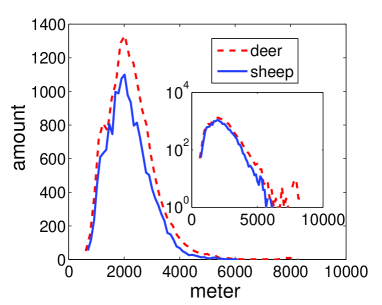
Figure 1: The frequency distribution of sum of walk distances in a day for deer and sheep. The data were obtained at the Macaulay Institute’s Glensaugh Research Station, Aberdeenshire, in north-east Scotland. By equipping each one of 20 red deer and 14 sheep with a GPS collar receiver instrument, which is fixed to the neck of the animals, the data of locations during a total time period of 140 days were collected every 30 or 60 minutes. Both distributions are very narrow and decay exponentially (subplots), which represents the energy distribution is homogenous.

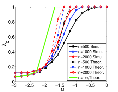
Figure 2: The simulated and analytical dependence of $\lambda_{c}$ on $\alpha$ under $w=10$. It shows the critical threshold $\lambda_{c}$ obtained by the numeric simulation model and reaction equations under different exponent $\alpha$. Green line shows the analytical critical threshold represented by Eq. (8). As shown in Eq. (8), there is a phase transition on $\alpha=-2$. When $\alpha\geq-2$, the epidemic threshold burst mounting up into $1$, and when $\alpha<-2$, the epidemic threshold is small values. Because when $n\rightarrow+\inf$, it is very hard to calculate $\lambda_{c}$ around -2. We use a line to represent in the very small region around -2.

For many epidemics such as HIV, if one is infected, he/she cannot be cured and always has a possibility to infect others. While with many other extremely rapid spreading epidemics such as H1N1 and SARS, we always ignore them or have no antibiotics to control them at the very beginning of spreading. In these conditions, SI model is a reasonable model to study the spreading process. There is only one difference between SIS and SI model. In SIS model, an infected node will have a probability to become susceptive, while, in SI model, when a node is infected, it cannot be cured and always will infect other susceptive nodes. According to the outbreaks of H1N1 and SARS, we know that there are always a few infected individuals and even only one infected individual in some cases. So, in the following numerical experiments, we preset only one node to be infected at the beginning and the effective spreading rate $\lambda=0.05$ always.

The spreading processes are simulated on networks with different network size. At first, we investigate the dependence of infected ratio on spreading time. As shown in Fig. 3, we can see that when $\alpha=-2$, the epidemic spread fastest under each network size. Then, we also studied the dependence of terminal time $T$ (at $T$, all nodes are infected) on $\alpha$ and we find that when $w$ is not too large, $T$ achieves the lowest value around the point of $\alpha=-2$ (shown in Fig. 4). Moreover for not too large energy $w$, $T\propto n^{\beta}$. When $\alpha=-2$, $\beta\approx\frac{1}{2}$ (shown in Fig. 5).

In the spatial weighted network, the spreading process is the most efficient when $\alpha=-2$. Can we get a similar conclusion in the cases of higher dimensional? It is still an open question because it seems tough to explain why epidemic spreading is fastest when $\alpha=-2$ by using strict mathematical analysis, and the numeric simulations on high-dimensional networks are too expensive to do. However, we speculate this conclusion can be extended to the cases of higher dimensional. Recent studies have presented that, with the constraint $W=wn$, the average shortest path length $D$ also achieves the lowest value when $\alpha=-2$ Hu ; Halvin . So, we investigate the relationship between terminal time $T$ and the average shortest path length $D$. However, it is not convenient to obtain the average shortest path length for the spatial weighted network. The reason is that large $w_{ij}$ means node $i$ and $j$ are very close, that is to say, we have to transform this kind of weight if we want to obtain the shortest path which is of great importance to us. In order to avoid transformation, we construct another un-weighted network which is similar to spatial weighted network. Based on a given uniform cycle network, we randomly add connections which hold the above constraint and by avoiding duplicated link to obtain an un-weighted network. By observing all phenomena detected on the above spatial weighted network, we find that the average shortest path length $D$ indeed affects the spreading speed almost linearly, shown as in Fig. 6 and Fig. 7, although, the slops at the two sides of $\alpha=-2$ are slight different. This difference implies that there are some other factors which also affect the spreading speed besides the average shortest path length. We believe that in high-dimensional networks with Levy flights spatial structure, the epidemic also spreads fastest when $\alpha=-2$. In the future we will try our best to solve the question.

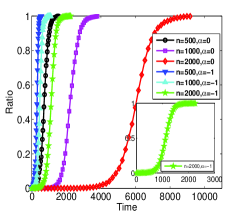
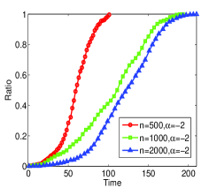
A        B

Figure 3: The dependence of spread ratio on time under different $\alpha$. A. Spread ratio under $\alpha=0$ and $\alpha=-1$, respectively. B. Spread ration under $\alpha=-2$. We can see that when $\alpha=-2$, the spread ratio grows much faster than other cases.

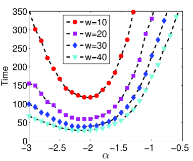
Figure 4: The dependence of terminal time $T$ on $\alpha$ under $n=1000$. It shows when the energy $w$ is not too large, the terminal time $T$ achieves the lowest value around the point of $\alpha=-2$, while the optimal $\alpha$ will deviate $-2$ and become smaller when $w$ is very large.

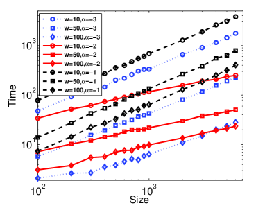
Figure 5: The dependence of terminal time $T$ on network size $n$. It observes the impact of network size on terminal time under various exponent $\alpha$ and energy $w$. There is a log-log linear dependence between terminate time and the network size. Move over we find that, for not too large energy $w$, $T\propto n^{\beta}$. When $\alpha=-2,\beta\approx\frac{1}{2}$.

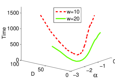
Figure 6: The relationship among the terminate time $T$, the average shortest path $D$ and Levy flights exponent $\alpha$. The lowest point of the curve is close at $\alpha=-2$, at this point the average shortest path and the terminate time are both the minimum value.

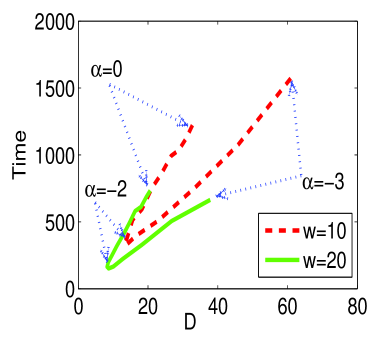
Figure 7: The dependence of terminate time $T$ on average shortest path $D$ under $n=2000$ with energy $w=10$ and $w=20$, the curve shown the $T$ reach the minimum value when $D$ touch the lowest point. Especially, when $\alpha>-2$, there is a linear relationship between $D$ and $T$.

IV Discussion and Conclusion

In summary, this paper presents the relationship between epidemic spreading and the mobility pattern of human and animal from the network perspective. Acknowledging that the mobility pattern of human and animal follows the Levy flights pattern with an exponent $\alpha\cong-2$, we find that the Levy flights mobility pattern is very efficient for epidemic spreading when $\alpha=-2$. This result presents a big challenge for epidemics control nowadays. On the other hand, this result in a sense complies with the evolution theory. The special mobility pattern has evolved since animal appeared on the earth. Maybe it is very useful for searching foods, diffusing good genes or many others which are very important for species developing. Consequently, it provides an effective path to spread epidemic. So it is of no surprise to obtain such a conclusion.

Acknowledgement.We wish to thank Prof. Shlomo Havlin and Prof. Tao Zhou for some useful discussions. The work is partially supported by NSFC under Grant No. 70771011 and 60774085. Y.Hu was supported by the BNU excellent Ph.D Project.

References

- (1) S. Boccaletti, V. Latora, Y. Moreno, M. Chavez, and D. U. Hwang. Physics Reports. 424: 175-308 (2006).
- (2) M. E. J. Newman. Phys. Rev. E. 66: 016128 (2002).
- (3) T. Zhou, Zhong-Qian Fu, Bing-Hong Wang. Progress in Natural Science. 16(5): 452-457 (2006).
- (4) M. E. J. Newman, S. Forrest, and J. Balthrop. Phys. Rev. E. 66: 035101 (2002).
- (5) P. M. A. Sloot, C. Boucher. et al. Int. J. Comput. Math. 85: 1175-1187 (2008).
- (6) D. H. Zanette. Phys. Rev. E. 65: 041908 (2002).
- (7) D. Balcan et al. BMC Medicine 7:45 (2009).
- (8) M. Kuperman, G. Abramson. Phys. Rev. Lett. 86:2902 (2001).
- (9) R. Pastor-Satorras, A. Vespignani. Phys. Rev. Lett. 86: 3200-3203 (2001).
- (10) R. Pastor-Satorras, A. Vespingnani. Phys. Rev. E. 63: 066117 (2002) .
- (11) R. Pastor-Satorras, A. Vespingnani. The Europhys. Jour. B. 26: 521-529 (2002).
- (12) D. W. Sims, J. D. Metcalfe. et al. Nature. 451: 1098-1102 (2008).
- (13) D. Brockmann, L. Hufnagel, and T. Geisel. Nature. 439:462-465 (2006).
- (14) M. C. Gonzalez, C. A. Hidalgo, and A.-L. Barabasi. Nature. 453: 779-782 (2008).
- (15) G. M. Viswanathan, H. E. Stanley. et al. Physica A. 282: 1-12 (2000).
- (16) H. Yang, et al. arXiv: 0908.3968
- (17) G. Li, et al. (2009) Designing optimal transport networks. arXiv: 0908.3869.