A simpel and versatile cold-atom simulator of Non-Abelian gauge potentials

Abstract

We show how a single, harmonically trapped atom in a tailored magnetic field can be used for simulating the effects of a broad class of non-abelian gauge potentials. We demonstrate how to implement Rashba or Linear-Dresselhaus couplings, or observe Zitterbewegung of a Dirac particle.

Simulating complex quantum systems with the help of trapped cold atoms has become a flourishing branch of quantum optics. The exquisite control and complex internal structure of cold atoms have allowed successful experimental simulation of systems and effects ranging from quantum phase transitions in the Bose-Hubbard model Greiner et al. (2002), over Anderson localization Billy et al. (2008); Roati et al. (2008), to cosmological models Leonhardt and Piwnicki (2000). Recently, a lot of research efforts have been directed towards realization of Abelian or Non-Abelian gauge fields. By bathing an optical lattice in additional weak, non-resonant light that can create Raman-transitions between hyperfine levels, one can create artificial magnetic fields which can be extremely strong. Vortex formation in a BEC has been observed due to such artificial magnetic fields Lin et al. (2009). Even the creation of magnetic monopoles has been proposed Pietilä and Möttönen (2009). Non-abelian gauge fields can be useful for studying spin-tronics materials with various spin-orbit couplings, Berry phases, or topologically protected qubits.

Most of these quantum simulations have been proposed or performed for atoms trapped in an optical lattice or Bose-Einstein condensates, requiring rather sophisticated experimental setups. Many physical systems are, however, interesting as single-particle systems. Such is the case e.g. for Anderson localization, the low-energy behavior of electrons in Graphene, or the relativistic motion of electrons that leads to the effect of Zitterbewegung Schrödinger (1930). It would be highly desirable to have a simple, versatile system that allows to simulate such single particle dynamics. We show here that such a system can be constructed from a single, harmonically trapped atom exposed to a suitably tailored real (physical) magnetic field. We show that by simply changing some gradients of different field components different non-Abelian gauge fields can be simulated, giving rise, for example, to Rashba or linear Dresselhaus coupling. We also show that Zitterbewegung should be easily observable. Abelian gauge fields can also be obtained, but are less interesting in the proposed setup, as they do not depend on position.

Consider a single atom of mass $m$ trapped in a harmonic potential (frequency $\omega$) and exposed to a magnetic field ${\bf B}({\bf x},t)$. For concreteness, let us assume a neutral atom in an optical dipole trap. The magnetic field should not be used for any part of the trapping, but be controllable independently of the trapping. We will also assume that the atom is cooled close to the ground state such that approximating the trap by a harmonic potential in all three directions is indeed reasonable. The hamiltonian of the system reads

$$H=\frac{{\bf p}^{2}}{2m}+\frac{1}{2}m\omega^{2}{\bf x}^{2}+g_{J}\mu_{B}{\bf B}({\bf x},t)\cdot{\bf J}/\hbar\,,$$ (1)

where $g_{J}$, $\mu_{B}$, and ${\bf J}$ are the g-factor, Bohr-magneton, and total angular momentum of the atom, and we have neglected the nuclear spin contribution in the Zeeman term. Suppose that the magnetic field varies slowly on the scale of the trapping potential, such that we can expand it in a power series about the origin ${\bf x}=0$,

$${\bf B}({\bf x},t)={\bf B}({\bf 0},t)+\sum_{i=1}^{3}\nabla B_{i}\cdot{\bf x}\,\hat{e}_{i}+{\cal O}({\bf x}^{2})\,,$$ (2)

with unit vectors $\hat{e}_{i}$ in directions $i=1,2,3\equiv x,y,z$. We have neglected higher order terms starting with the second order. One can still include the second order, with consequences to be discussed below, but for the moment suppose that the magnetic field varies slowly enough over the length-scale of the atomic motion in the trap that the quadratic term in ${\bf x}$ from expanding ${\bf B}$ can indeed be neglected compared to the quadratic term describing the trapping potential.

The linear term in ${\bf x}$ then leads to a coupling ${\bf x}\cdot\nabla({\bf B}\cdot{\bf J})\equiv{\bf x}\cdot\sum_{i}(\nabla B_{i}\left.\right|_{{\bf x}={\bf 0}})J_{i}$. Now let us canonically transform ${\bf x}/x_{0}\rightarrow-{\bf p}/p_{0}$, ${\bf p}/p_{0}\rightarrow{\bf x}/x_{0}$, where I have introduced the natural scales $x_{0}$ and $p_{0}$ of the canonical coordinates and momenta of the atom in the trap, $x_{0}=\sqrt{\hbar/(m\omega)}$ and $p_{0}=\sqrt{\hbar m\omega}$. The harmonic oscillator part in the hamiltonian is invariant under this transformation, but the ${\bf x}$ in the Zeeman term becomes a $-{\bf p}$, and we get the transformed hamiltonian $\tilde{H}$,

$$\tilde{H}=\frac{{\bf p}^{2}}{2m}+\frac{1}{2}m\omega^{2}{\bf x}^{2}-\frac{e}{m}{\bf p}\cdot{\bf A}+g_{J}\mu_{B}{\bf B}({\bf 0},t)\cdot{\bf J}/\hbar\,,$$ (3)

with

$${\bf A}=\frac{\mu_{B}g_{J}}{e\hbar\omega}\nabla\left({\bf B}\cdot{\bf J}\right)_{{\bf x}={\bf 0}}\,.$$ (4)

Note that ${\bf A}$ is independent of position and thus commutes with ${\bf p}$. We can therefore rewrite the hamiltonian in the form

$$\tilde{H}=\frac{1}{2m}({\bf p}-e{\bf A})^{2}+\frac{1}{2}m\omega^{2}{\bf x}^{2}+\phi+\mu_{B}g_{J}{\bf B}({\bf 0},t)\cdot{\bf J}/\hbar\,,$$ (5)

which makes appear ${\bf A}$ as a gauge potential. The constant $\phi$ acts only in the angular–momentum Hilbert space,

$$\phi\equiv-\frac{e^{2}{\bf A}^{2}}{2m}\,,$$ (6)

and can be considered an anisotropy for the angular momentum. We can write it as

$$\phi=-\frac{1}{2}{\bf J}^{t}I^{-1}{\bf J}\,,$$ (7)

where the inverse tensor of inertia $I^{-1}$ has matrix elements

$$(I^{-1})_{ij}=\frac{\mu_{B}^{2}g_{J}^{2}}{m\hbar^{2}\omega^{2}}\nabla B_{i}\cdot\nabla B_{j}\,.$$ (8)

The effect created by the gauge potential plays an appreciable role only if the components of $e{\bf A}$ are comparable to the corresponding components of ${\bf p}$. The latter are, close to the ground-state of the harmonic potential, of the order of $p_{0}$. With ${\bf J}\sim\hbar$, we are thus led to a condition for the magnitude of the magnetic field gradient $B^{\prime}$

$$B^{\prime}\sim\frac{\sqrt{\hbar m}\omega^{3/2}}{\mu_{B}}\,,$$ (9)

which should be satisfied for at least one component of ${\bf B}$. Inserting the data for ⁸⁷Rb, we find a gradient $B^{\prime}=2.1$Gauss/mm for $\omega=2\pi\cdot$1kHz, which appears to be a very convenient order of magnitude.

It is worthwhile spelling out the components of ${\bf A}$ explicitly. Up to the common prefactor $\frac{\mu_{B}g_{J}}{e\hbar\omega}$ we have

$${\bf A}_{x} \propto \partial_{x}B_{x}\,J_{x}+\partial_{x}B_{y}\,J_{y}+\partial_{x}B_{z}\,J_{z}$$ (10)

$${\bf A}_{y} \propto \partial_{y}B_{x}\,J_{x}+\partial_{y}B_{y}\,J_{y}+\partial_{y}B_{z}\,J_{z}$$ (11)

$${\bf A}_{z} \propto \partial_{z}B_{x}\,J_{x}+\partial_{z}B_{y}\,J_{y}+\partial_{z}B_{z}\,J_{z}\,.$$ (12)

The components of ${\bf J}$ are real physical angular momentum, and thus satisfy $[J_{x},J_{y}]=i\hbar J_{z}$ in any Hilbert space. Therefore, obviously, the gauge field is in general non-abelian. The remarkable thing about ${\bf A}$ is that it is easily programmable by an appropriate choice of magnetic field gradients. Choosing for instance only a field gradient of one magnetic field component leaves us with only one component of the angular momentum and we thus get an abelian gauge potential. Choosing arbitrary linear combinations of angular momentum operators is only restricted by the properties of the real physical magnetic field employed, in particular ${\rm div}{\bf B}=0$, as we shall see below.

Before working out a few specific examples, three more remarks:

1. We chose the same trap frequency $\omega$ in all directions, which is certainly somewhat unusual for an optical dipole trap. After canonical transformation, this translates into the same mass for all three directions. Had we different trap frequencies in different directions, we would get effectively different masses in different directions, i.e. a (diagonal) effective mass tensor, similar to the situation in a semiconductor. This may or may not be useful, depending on what one wants to simulate.

2. Similarly, if we kept the quadratic term in the expansion of ${\bf B}$, we would get additional quadratic terms (which would also depend on the internal state of the atom) contributing to the trapping potential, such that, again, after the canonical transformation we would end up with different masses in different directions.

3. What was derived here for a single atom should translate immediately to a BEC, if the interactions between atoms are negligible. If they are not, any interaction potential $V({\bf x}_{i}-{\bf x}_{j})$ will translate into a momentum dependent interaction after the canonical transformation.

Let us now look at some concrete examples of non-Abelian gauge potentials, inspired by the list in Vaishnav and Clark (2008). I will assume that we have an atom with $J=1/2$, so that the $J_{i}$ are given by Pauli-matrices, $J_{i}=(\hbar/2)\sigma_{i}$.

Rashba coupling. This is a coupling $\alpha(p_{y}\sigma_{z}-p_{z}\sigma_{y})$, with some constant $\alpha$. It can easily be achieved by choosing $\partial_{x}B_{i}=0$, for $i=x,y,z$, $\partial_{y}B_{y}=0=\partial_{z}B_{z}$, and $\partial_{y}B_{z}=B^{\prime}=\partial_{z}B_{y}$. No magnetic mono-pole is required, ${\rm div}{\bf B}=0$, but the field has a finite curl in $x$-direction, $(\nabla\times{\bf B})_{x}=2B^{\prime}$. That curl is needed at ${\bf x}={\bf 0}$, where we did the expansion of the magnetic field. But since we insisted on a linearly growing field over the lengthscale of the motion in the trap, we request basically circular magnetic field lines around the $x$-axis, with magnetic field strength growing linearly with distance from the $x$-axis. That is, of course, quite different from what a current carrying wire along the $x-$axis would do (apart from the fact that that wire would have to go straight through ${\bf x}=0$, where we would like to trap the atom). A possible way of creating the required magnetic field might be through an electric field that increases linearly in time by using segmented cylindrically arranged electrodes. Choosing the right voltage profile for all the electrodes one can create a radially symmetric electric field oriented in $x$-direction that increases proportionally in radial direction, and generates the desired ${\bf B}$-field according to Maxwell’s equation $\nabla\times{\bf H}=\dot{{\bf D}}+{\bf j}$.

The inverse tensor of inertia is here simply $I^{-1}={\rm diag}(0,B^{\prime 2},B^{\prime 2})$ and just leads to a constant $\phi=B^{\prime 2}{\bf 1}$, i.e. an identity matrix in spin Hilbert–space.

Linear Dresselhaus coupling. Here we want $A_{y}=\alpha\sigma_{y}$, $A_{z}=-\alpha\sigma_{z}$. Choose again $\partial_{x}B_{i}=0$ $\forall i$, but then $\partial_{y}B_{y}=B^{\prime}=-\partial_{z}B_{z}$, and all other derivatives equal zero. Again, this is compatible with ${\rm div}{\bf B}=0$, and we basically get a field that is point symmetric, growing linearly in radial direction, but pointing towards the center on the $z-$axis and outward on the $y-$axis, like from a quadrupole magnet.

Inverse tensor of inertia and the resulting potential $\phi$ are identical to the Rashba case.

Graphene sheet in vicinity of Dirac point. This case is more problematic: we want $A_{y}=\alpha\sigma_{y}$, $A_{z}=\alpha\sigma_{z}$, which leads to $\partial_{y}B_{y}=B^{\prime}=\partial_{z}B_{z}$. But ${\rm div}{\bf B}=0$ then requires $\partial_{x}B_{x}=-2B^{\prime}$, and thus adds an extra coupling term $-2p_{x}\sigma_{x}$ to the desired $p_{y}\sigma_{y}+p_{z}\sigma_{z}$.

Zitterbewegung. Zitterbewegung (ZB) is an interference effect first predicted by Schrödinger for relativistic spin-1/2 particles that leads to a jittering motion on the length scale of the Compton wavelength of the particle, i.e. $h/mc\simeq 10^{-12}$m for an electron Schrödinger (1930). This short length scale has so far prevented direct experimental observation of ZB for relativistic electrons. However, the effect should exist for any spinor system with linear dispersion relation. Consequently, ZB has been studied theoretically in several systems, including mesoscopic wires Schliemann et al. (2005), graphene Cserti and Dávid (2006), ion traps Lamata et al. (2007), and optical lattices Vaishnav and Clark (2008). Rashba couplings in quantum dots with rotationally invariant potentials in 2D was studied in Tsitsishvili et al. (2004). Very recently, ZB was observed experimentally with a single trapped ion Gerritsma et al. (2009). ZB has mostly been studied for a free particle. The ZB then dies out after a short time, when the two wave-packages corresonding to spin-up and spin-down have separated enough to prevent further interference. It is interesting to consider how the additional harmonic confinement potential in (5) modifies the ZB. One might expect that the confinement will increase the time interval in which the ZB can be observed.

We now study ZB for the harmonic confinement (5) in the Rashba case. We show that ZB exists even if the harmonic oscillator is initially unexcited, and that it can persist for arbitrarily long times. Note that the third direction, $x$ in the above notation, is not affected by the gauge field and just separates. It is convenient then, to rewrite (5) in terms of annihilation (creation) operators $a(a^{\dagger})$ and $b(b^{\dagger})$ for the $y$ and $z$ components, respectively. We are thus lead to

$$H = \hbar\omega\left(a^{\dagger}a+b^{\dagger}b+ib_{1}\big{(}-(a-a^{\dagger})\sigma_{z}+(b-b^{\dagger})\sigma_{y}\right)$$ (13)

$$+{\bf b}_{0}\cdot\mbox{\boldmath{$\sigma$}}\big{)}\,,$$

where the dimensionless parameters are $b_{1}=\frac{g_{J}\mu_{B}B^{\prime}}{2\sqrt{\hbar m\omega^{3}}}$ and ${\bf b}_{0}=\frac{\mu_{B}g_{J}{\bf B}(0)}{2\hbar\omega}$, and we have suppressed an irrelevant constant.

It is straightforward to express $H$ in basis states $|nms\rangle$, where $n,m\in\{0,1,2,\ldots\}$ are the occupation numbers for oscillators $a$ and $b$, and $s\in\{\pm 1\}$ label eigenstates of $\sigma_{z}$ corresponding to these eigenvalues, and to diagonalize the Hamiltonian numerically. This basis turns out to be highly suitable — taking into account only up to 5 excitations per oscillator (i.e. a 72 dimensional basis) allows one to find the lowest 26 eigenstates already with 4 significant digits for $b_{1}=0.1$ (compared to the case with 10 excitations per oscillator, or 242 basis states, which we used in the numerical simulations). With the obtained propagator we can study the time evolution of the averages of the observables $\langle y(t)\rangle$, $\langle p_{y}(t)\rangle$ etc.

Figure 1 shows $\langle y(t)\rangle$ for ${\bf b}_{0}={\bf 0}$, different values of $b_{1}$, and the two initial states $|\psi(0)\rangle=|00+\rangle$ and $|00-\rangle$. Both $\langle z(t)\rangle$ and $\langle p_{z}(t)\rangle$ remain always zero in these cases, whereas $\langle y(t)\rangle$ shows oscillations. They are always with opposite sign for these two different initial states. For small values of $b_{1}$ ($b_{1}=0.1$) the oscillations appear periodic, whereas with increasing $b_{1}$, additional harmonics appear that make the signal look more and more erratic. By changing the initial state of the spin, the direction of the oscillation can be chosen. E.g. for$|\psi(0)\rangle=(|00+\rangle+i|00-\rangle)/\sqrt{2}$, we obtain $\langle y(t)\rangle=0=\langle p_{y}(t)\rangle$, whereas the $z$-component now shows the signal we had for $\langle y(t)\rangle$. The state $|\psi(0)\rangle=(\cos(\pi/8)|00+\rangle+i\sin(\pi/8)|00-\rangle)$ leads to oscillations with $\langle y(t)\rangle=-\langle z(t)\rangle$. It appears thus that the ZBis always one-dimensional as long as the initial state is chosen in the subspace $\{|00+\rangle,|00-\rangle\}$. The superposition $|\psi(0)\rangle=(|00+\rangle+|00-\rangle)/\sqrt{2}$ switches the ZB off in both components. Note that one-dimensional ZB was also predicted for a 1D harmonic confinement and a specific initial spin state, with the ZB perpendicular to the free 1D motion Schliemann et al. (2005).

The results for small $b_{1}$ can be easily understood analytically, by going to the Heisenberg picture and expanding the time dependent operators to lowest order in $b_{1}$. We find, correct to order ${\cal O}(b_{1})$, at ${\bf b}_{0}={\bf 0}$

$$\langle y(t)\rangle \simeq \langle y(0)\rangle\cos\omega t+\langle p_{y}(0)\rangle\sin\omega t$$ (14)

$$+\sqrt{2}b_{1}\langle\sigma_{z}(0)\rangle\sin\omega t$$

$$\langle z(t)\rangle \simeq \langle z(0)\rangle\cos\omega t+\langle p_{z}(0)\rangle\sin\omega t$$ (15)

$$-\sqrt{2}b_{1}\langle\sigma_{y}(0)\rangle\sin\omega t$$

$$\langle p_{y}(t)\rangle \simeq \langle p_{y}(0)\rangle\cos\omega t-\langle y(0)\rangle\sin\omega t$$ (16)

$$+\sqrt{2}b_{1}\langle\sigma_{z}(0)\rangle(\cos\omega t-1)$$

$$\langle p_{z}(t)\rangle \simeq \langle z(0)\rangle\cos\omega t-\langle z(0)\rangle\sin\omega t$$ (17)

$$-\sqrt{2}b_{1}\langle\sigma_{y}(0)\rangle(\cos\omega t-1)\,.$$

All positions and momenta are expressed in terms of the length-scales $x_{0}$ and momentum scales $p_{0}$ of the harmonic oscillator, respectively. The corrections to Eqs.(14-17) are of order ${\cal O}(B_{1}^{2})$. We recognize in the terms independent of $b_{1}$ the unperturbed motion of the 2D harmonic oscillator. This motion can be switched off by chosing average initial positions and momenta equal zero, as is the case for the initial states discussed above with the two harmonic oscillators initially in their ground state. All motion is then entirely due to the ZB and indeed 1D, in a direction given by the vector $(\langle\sigma_{z}(0)\rangle,\langle\sigma_{y}(0)\rangle)$. Interestingly, at $|b_{1}|\ll 1$ the ZB is itself harmonic with an amplitude controlled by $b_{1}$. The fact that the length and momenta scales of the ZB are set by the harmonic confinement should allow for a much simpler experimental verification than for Dirac electrons. Moreover, the harmonic confinement potential keeps the wavepackages corresponding to the two different spin components together, preventing the decay of the ZB, which should facilitate its experimental study. A damping of the ZB can arise at higher values of $b_{1}$ and initial coherent states of the harmonic oscillators, which will in general be smeared out due to the anharmonicity mediated by the coupling to the spin (see Figs.2 and 3). At $b=1$ the dynamics looks random and diffusive in the $yz$-plane, but the trajectory of average values $(\langle y(t)\rangle,\langle z(t)\rangle)$ is of course entirely deterministic and reproducible.

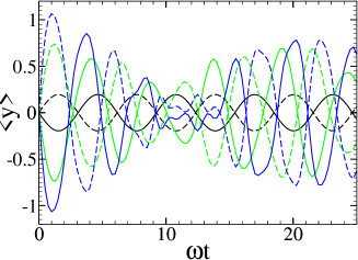
Figure 1: (Color online) Zitterbewegung in $\langle y(t)\rangle$ (in units of harmonic oscillator length $x_{0}$) for initial states $|00+\rangle$ (full lines) and $|00-\rangle$ (dashed lines); ${\bf b}_{0}={\bf 0}$, and $b_{1}$ takes the values $b_{1}=0.1$, $0.5$ and 1 for black lines, green (light grey) lines, and blue lines (dark grey), respectively.

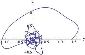
Figure 2: (Color online) Trajectory of 2D Zitterbewegung in $(\langle y(t)\rangle,\langle z(t)\rangle)$ (in units of harmonic oscillator length $x_{0}$) for an initial state $|\alpha\beta+\rangle$, where $|\alpha\rangle$ and $|\beta\rangle$ are coherent states with $\alpha=1$ and $\beta=i$ at ${\bf b}_{0}={\bf 0}$ and $b_{1}=1$. The trajectory is shown for $0\leq\omega t\leq 50$. The initial state is localized at $\langle y(0)\rangle=\sqrt{2}=\langle p_{z}(0)\rangle$, $\langle z(0)\rangle=0=\langle p_{y}(0)\rangle$ and would lead for $b_{1}=0$ to circular motion in the $yz$-plane.

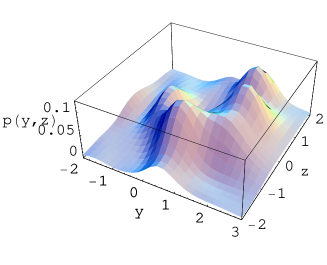
Figure 3: (Color online) Probability distribution $p(y,z)$ of finding the atom localized at position $y,z$ (in units of $x_{0}$) at $\omega t=10$, for $b_{1}=1.0$, ${\bf b}={\bf 0}$. The initial coherent state (same state as in Fig.2) gets smeared out due to the anharmonicity created by the Rashba coupling.

Figure 4: Lowest $20$ energies in the Spectrum of $H$ in units of $\hbar\omega$ as function of $b_{1}$ at ${\bf b}_{0}={\bf 0}$. The spectrum is symmetric under $b_{1}\to-b_{1}$, and each energy level shown is still doubly degenerate.

The increasingly erratic behavior of the ZB with increasing $b_{1}$ can be understood by looking at the spectrum of $H$, plotted in Fig.4. The oscillator states at $b_{1}=0$ containing $n$ energy quanta which are $2(n+1)$–fold degenerate (states $|n0+\rangle$, $|n-1\,1+\rangle,\ldots,|0n+\rangle$, and the same set once more but with spin down). They split with increasing $b_{1}$ and lead to several avoided crossings. The resulting incommensurate frequencies lead to the observed quasi-periodic, apparently random behavior.

In summary, we have shown how a single trapped atom with hyperfine structure trapped in a magnetic field with suitably tailored field gradients can be used to simulate the effect of non-abelian gauge potentials. We have demonstrated how different effective spin-orbit couplings (such as Rashba or linear Dresselhaus couplings) can be easily obtained, and we have proposed a new way of observing Zitterbewegung of a harmonically trapped particle. An immediate consequence of the fact that (5) was obtained by a canonical transformation that exchanges position and momentum, is that the ZB in $y(t)$ will, of course, show up in $p_{y}(t)$ in the original system. The simplicity and flexibility of the proposed setup may also allow the study of other spin-orbit couplings, as well as of applications such as robust quantum gates based on topological phases Kitaev .

Acknowledgements: I would like to thank the JQI (University of Maryland and NIST Gaithersburg) for hospitality during my stay during which this work was started, and Victor Galitski, Trey Porto, Bill Phillips, Ian Spielman, and Jay Vaishnav for discussions.

References

- Greiner et al. (2002) M. Greiner, O. Mandel, T. Esslinger, T. W. Hänsch, and I. Bloch, Nature 415, 39 (2002).
- Billy et al. (2008) J. Billy, V. Josse, Z. Zuo, A. Bernard, B. Hambrecht, P. Lugan, D. Clement, L. Sanchez-Palencia, P. Bouyer, and A. Aspect, Nature 453, 891 (2008), ISSN 0028-0836, URL http://dx.doi.org/10.1038/nature07000.
- Roati et al. (2008) G. Roati, C. D/’Errico, L. Fallani, M. Fattori, C. Fort, M. Zaccanti, G. Modugno, M. Modugno, and M. Inguscio, Nature 453, 895 (2008), ISSN 0028-0836, URL http://dx.doi.org/10.1038/nature07071.
- Leonhardt and Piwnicki (2000) U. Leonhardt and P. Piwnicki, Physical Review Letters 84, 822 (2000), ISSN 0031-9007, URL http://prl.aps.org/abstract/PRL/v84/i5/p822_1.
- Lin et al. (2009) Y. Lin, R. L. Compton, K. Jimenez-Garcia, J. V. Porto, and I. B. Spielman, Nature 462, 628 (2009), ISSN 0028-0836, URL http://dx.doi.org/10.1038/nature08609.
- Pietilä and Möttönen (2009) V. Pietilä and M. Möttönen, Phys. Rev. Lett. 103, 030401 (2009).
- Schrödinger (1930) E. Schrödinger, Die Naturwissenschaften 24, 418 (1930).
- Vaishnav and Clark (2008) J. Y. Vaishnav and C. W. Clark, Physical Review Letters 100, 153002 (pages 4) (2008), URL http://link.aps.org/abstract/PRL/v100/e153002.
- Schliemann et al. (2005) J. Schliemann, D. Loss, and R. M. Westervelt, Phys. Rev. Lett. 94, 206801 (2005).
- Cserti and Dávid (2006) J. Cserti and G. Dávid, Phys. Rev. B 74, 172305 (2006).
- Lamata et al. (2007) L. Lamata, J. León, T. Schätz, and E. Solano, Phys. Rev. Lett. 98, 253005 (2007).
- Tsitsishvili et al. (2004) E. Tsitsishvili, G. S. Lozano, and A. O. Gogolin, Physical Review B (Condensed Matter and Materials Physics) 70, 115316 (pages 11) (2004), URL http://link.aps.org/abstract/PRB/v70/e115316.
- Gerritsma et al. (2009) R. Gerritsma, G. Kirchmair, F. Zähringer, E. Solano, R. Blatt, and C. F. Roos, 0909.0674 (2009), URL http://arxiv.org/abs/0909.0674.
- (14) A. Kitaev, eprint quant-ph/9511026.