Gravitational lensing in the Supernova Legacy Survey (SNLS).

Abstract

Aims. The observed brightness of Type Ia supernovae is affected by gravitational lensing caused by the mass distribution along the line of sight, which introduces an additional dispersion into the Hubble diagram. We look for evidence of lensing in the SuperNova Legacy Survey 3-year data set.

Methods. We investigate the correlation between the residuals from the Hubble diagram and the gravitational magnification based on a modeling of the mass distribution of foreground galaxies. A deep photometric catalog, photometric redshifts, and well established mass luminosity relations are used.

Results. We find evidence of a lensing signal with a $2.3\,\sigma$ significance. The current result is limited by the number of SNe, their redshift distribution, and the other sources of scatter in the Hubble diagram. Separating the galaxy population into a red and a blue sample has a positive impact on the significance of the signal detection. On the other hand, increasing the depth of the galaxy catalog, the precision of photometric redshifts or reducing the scatter in the mass luminosity relations have little effect. We show that for the full SuperNova Legacy Survey sample ($\sim$400 spectroscopically confirmed Type Ia SNe and $\sim$200 photometrically identified Type Ia SNe), there is an 80% probability of detecting the lensing signal with a 3 $\sigma$ significance.

1 Introduction

Type Ia supernovae (SNe Ia) have become an essential tool of observational cosmology (Riess et al., 1998; Perlmutter et al., 1999; Astier et al., 2006; Wood-Vasey et al., 2007; Riess et al., 2007; Freedman et al., 2009; Kessler et al., 2009). By studying the distance-redshift relation of a large number of SNe Ia over a wide range in redshift, the equation of state of dark energy can be measured. Although SNe Ia can be calibrated to be good standard candles, they are affected by systematic effects such as extinction by dust and gravitational lensing. Because of gravitational lensing, most supernovae will be slightly demagnified and some will be significantly magnified due to the mass inhomogeneities along the line of sight.

This causes an additional dispersion in the observed magnitudes and thus in the Hubble diagram. The effect is greater at high redshift, but is still less than the scatter in the Hubble diagram for a redshift up to 1, as we see in this paper.

Magnification of SNe Ia can be estimated in 2 ways. The Hubble diagram residuals, computed assuming the best fit cosmological model, give

an indirect measure of the SN magnification. The magnification can, on the other hand, also be estimated by

modeling the foreground galaxy mass distribution using galaxy photometric measurements together with derived mass-luminosity relations for galaxies and dark matter halo models. If a correlation between these two estimates is found, it could give interesting insight in the modeling of the mass distribution of the foreground galaxies. This will be discussed in another paper (Jönsson et al., 2009)

The lensing signature in supernovae samples has already been sought for. Williams & Song (2004) correlated the brightness of high-z supernovae from the High-z Supernova Search Team and the Supernova Cosmology Project with the density of the foreground galaxies. They found that brighter supernovae preferentially lay behind over-dense regions at a 99 % CL. However, they find a lensing contribution to the scatter in the Hubble diagram of 0.11 mag (for a median redshift below 0.5) which is larger than expected (for example from lensing statistics), as noted by the authors themselves. Ménard & Dalal (2005) remark that the measured size of the effect is also incompatible with shear variance measurements. Finally, such a large magnification effect would cause a significant increase of Hubble diagram scatter with redshift, undetected today. Wang (2005) derived the expected weak lensing signatures of Type Ia SNe by convolving the intrinsic distribution in peak luminosity with expected magnification distributions and compared the expected and measured skewnesses of the residual distribution of 110 high and low-z SNe from the Riess sample (Riess et al., 2004). The signal found is dominated by high redshift events uncorrected for the NICMOS non-linearity. Its origin remains unknown and its significance is not provided. Partly using the same supernova sample, Ménard & Dalal (2005) searched for a correlation using SDSS photometry of the foreground galaxies and found no evidence for a correlation. More recently Jönsson et al. (2007) found a weak correlation with a confidence level of $90\%$ using high-z supernovae from the GOODS fields. A firm detection of this effect therefore remains to be found.

The SNLS sample is currently the best suited sample for a possible detection of such a signal thanks to its large number of SNe Ia at high redshift (Jönsson et al., 2008).

In this paper, we investigate the possible correlation between the magnification of the SNLS SNe derived from photometric measurements of the foreground galaxies (together with chosen mass-luminosity relations) and the residuals from the Hubble diagram.

Evaluating the expected magnification by foreground galaxies can be schematically split into three steps : first obtaining redshifts and absolute magnitudes of the foreground galaxies, then converting these informations into mass, and finally turning this set of mass and redshift estimates into a magnification estimate.

The outline of the paper is as follows. $\S$2 introduces the mass-luminosity relations used in this analysis. In $\S$3 the SNLS 3-year data set is presented. $\S$4 describes the analysis steps to estimate the supernovae magnifications, while in $\S$5 we present the measured correlation and compare it with expectations from simulations. Finally, we summarize in $\S$6.

2 Mass Luminosity relations

There are several ways of inferring the combined mass of a galaxy and its dark matter halo using the measured luminosity. We make use of two approaches in this paper.

i) The line-of-sight velocity dispersions in elliptical galaxies and rotational velocities in spiral galaxies are correlated with their luminosities. Those are the well established Faber-Jackson (Poveda, 1961; Fish, 1964; Faber & Jackson, 1976) and Tully-Fisher (Tully & Fisher, 1977; Haynes et al., 1999) relations .

ii) Galaxy-galaxy lensing measurements allow a relation to be determined between luminosity and mass once a functional form is assumed for the mass density profile.

We present below recent results for these approaches and compare them assuming a Singular Isothermal Sphere dark matter density profile (hereafter SIS) which has proven to be a good fit to lensing galaxies (Koopmans et al., 2006).

2.1 Tully-Fisher relation for spiral galaxies

We have chosen to use the Boehm et al. (2004) results for the Tully-Fisher (TF) relation. The maximum rotational velocities of 77 spiral galaxies in a redshift range of $0.1<z<1.0$ were measured in the FORS Deep Field. Anchoring the TF relation at low $z$ using the results from Pierce & Tully (1992), they obtain the following relation between the maximum rotation velocity $v_{\rm max}$ and the absolute magnitude $M_{B}$ of the galaxy in the rest-frame $B$-band (in a Vega magnitude system):

$$\log v_{\rm max}=-0.134\left(M_{B}+(3.61\pm 0.24)+(1.22\pm 0.56)\cdot z\right)$$ (1)

The observed scatter of $M_{B}$ about this relation is $0.41$ mag (r.m.s.). The redshift dependence expresses the fact that a galaxy of a given mass was brighter in the past as it hosted a younger stellar population (Barden et al., 2003; Milvang-Jensen et al., 2003; Bamford et al., 2006; Chiu et al., 2008).

The maximum rotational velocity $v_{\rm max}$ of spiral galaxies, measured at large galactic radii, is dominated by the dark matter mass. Assuming a SIS dark matter density profile for which the rotational velocity is constant, we have $v_{\rm max}\simeq v_{\rm rot}(r\rightarrow\infty)=\sqrt{2}\sigma$, where $\sigma$ is the one-dimensional r.m.s. of the velocity distribution.

2.2 Faber-Jackson relation for elliptical galaxies

We adopt the Faber-Jackson relation (FJ) by Mitchell et al. (2005) (hereafter M05) derived for a sample of $\sim 30,000$ elliptical galaxies using SDSS data. The selection criteria for the sample and the estimate of the velocity dispersion are described in Bernardi et al. (2003). The observed velocity dispersion has been determined by analyzing the integrated spectrum of the whole galaxy and aperture corrected to a standard effective radius. M05 find the following relation between the velocity dispersion and the absolute magnitude $M_{r}$ of the galaxy in the rest-frame $r$-band (in a AB system):

$$<\log(\sigma)>=2.2-0.091(M_{r}+20.79+0.85z)$$ (2)

As for the TF relation, the redshift dependence accounts for the evolution of the age and hence luminosity of the stellar population. The scatter in the FJ relation induces an uncertainty in the estimate of the velocity dispersion which has been given by Sheth et al. (2003):

$$\mathrm{r.m.s.}(\log\sigma)=0.79(1+0.17(M_{r}+21.025+0.85z))$$

The measured velocity dispersions are aperture-corrected central velocity dispersions which are almost equal to the dark matter velocity dispersions (see ??), so we can identify those measurements with the velocity dispersion parameter of the SIS profile.

We choose to translate the FJ r-band relation into a restframe B-band relation since restframe B is covered with SNLS griz bands up to $z\simeq 1$. To convert the SDSS $r$-band absolute magnitudes in the AB system to standard $B$-band Vega absolute magnitudes, a typical color $M_{B}-M_{r}$ for ellipticals in the AB system is estimated yielding $M_{B}-M_{r}=1.20$ (Gunnarsson et al., 2006) and an AB to Vega relation $B_{\rm AB}=B_{\rm Vega}-0.12$ is adopted.

2.3 Galaxy-galaxy lensing mass estimates

The galaxy-galaxy lensing signal manifests itself by images of background (faint) galaxies being distorted by foreground (brighter) galaxies (Hoekstra et al., 2004, 2005; Parker et al., 2005; Kleinheinrich et al., 2006; Mandelbaum et al., 2006). Unfortunately, one can only study ensemble averaged properties because the weak-lensing distortion induced by an individual galaxy is too small to be detected. The measured quantity is the mean tangential shear which is proportional to the total lens galaxy-halo mass. Since the lensing signal depends on the angular diameter distance between observer, lens and source, galaxy-galaxy lensing results strongly depend on the properties of the galaxy sample, which differ for different surveys.

We use the galaxy-galaxy lensing result from Kleinheinrich et al. (2006) (hereafter K06). The data is taken from the COMBO-17 survey which consists of observations in five broad-band filters (UBVRI) and 12 medium-band filters. They report a mass to luminosity relation for the full sample probed out to a maximum radius of 150 h^-1kpc when modeling the lenses as SIS profiles:

$$\sigma=156^{+18}_{-24}\left(\frac{L}{10^{10}h^{-2}L_{r\odot}}\right)^{0.28^{+0.12}_{-0.09}}\mathrm{km}.\mathrm{s}^{-1}$$ (3)

where $L$ is the luminosity of the galaxy. The fiducial luminosity, $L^{*}=10^{10}h^{-2}L_{r\odot}$ is given in the SDSS $r$-band. For a conversion to the $B$-band, they have calculated that the galaxies in their sample with a fiducial luminosity of $L_{*}=10^{10}h^{-2}L_{B\odot}$ in the $B$-band have a fiducial luminosity of $L_{*}=1.1\times 10^{10}h^{-2}L_{r\odot}$ in the SDSS $r$-band. Note that for the SIS profile, the halo is characterized by its velocity dispersion which is the key parameter entering in the estimation of the magnification (see section 4.4).

2.4 Comparison assuming a Singular Isothermal Sphere profile

In Figure 1, we show the velocity dispersion as a function of absolute $B$-band magnitude for the three different mass-luminosity relations (Eq. 1,2,3 for TF, FJ relations and galaxy-galaxy lensing results of K06) assuming a SIS dark matter mass profile. The mean redshift of the lens galaxies in the K06-relation is $\sim 0.4$. For a given $B$-band luminosity, elliptical galaxies are more massive than spirals so the FJ relation naturally gives higher velocity dispersion than the TF relation. The K06 relation and the FJ relation appear quite similar. For high luminosity galaxies the difference in mass estimate from the three relations can lead to very different magnifications. As an example, for a bright galaxy of absolute magnitude M_B=-22, the velocity dispersions range from 170 km s^-1 (TF) to 249 km s^-1 (FJ) and 248 km s^-1 (K06). As a consequence, in order to obtain accurate estimates of the magnification it is important to take into account the galaxy type.

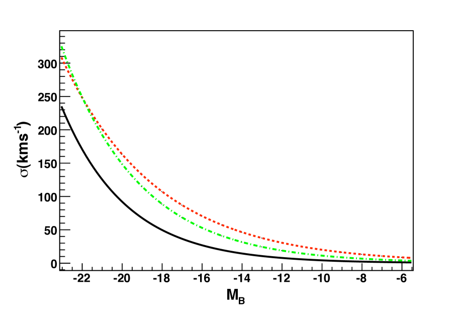
Figure 1: Velocity dispersions as a function of the absolute magnitude in the $B$-band for three different mass-luminosity relations at a redshift of $z=0.4$. In green (dash-dotted) the K06 relation, in red (dotted) the FJ relation and in black (solid) the TF relation. The plot shows the velocity dispersion in km s^-1 as a function of absolute magnitude in the $B$-band.

3 Data

The SuperNova Legacy Survey consists of an imaging survey which is part of the (deep component of the) Canada-France-Hawaii Telescope Legacy Survey and a spectroscopic survey done on 8m class telescopes. The imaging was done with the MegaCam imager (360 Megapixels, 1 deg²) which detects and monitors the light curves of the SNe, over four different fields of 1 deg² (called D1, D2, D3, D4). D1 overlaps partly with the VVDS survey, D2 with the COSMOS survey, and D3 with the DEEP2 survey. We will later use the spectroscopic galaxy redshifts from the DEEP2 and VVDS surveys to establish and test photometric galaxy redshifts.

The ”rolling” search method was used for the $griz$ bands, which means observing the same field every 3-4 days during dark and gray time (typically for a period of $\sim 16$ days around new moon) for as long as it remains visible (from 5 to 7 months a year). Images in $u$ are also used in this analysis. The images are used both to monitor the SN light curves and to build photometric catalogs of the objects in the fields, in particular the galaxies.

For each field, the total exposure times used to build the galaxy catalogs for this analysis amount to more than 20 h per band, reaching typically 60 hours in the $i$-band.

Spectroscopy of the supernovae is crucial in order to obtain redshifts, and to confirm the type of each supernova. The spectroscopic follow-up for the SNLS was done with the VLT (Baumont et al., 2008; Balland et al., 2009), Gemini (Howell et al., 2005; Bronder et al., 2008) and Keck telescopes (Ellis et al., 2008). The 3-year data set used in this paper consists of 233 spectroscopically confirmed Type Ia supernovae used for cosmological analyses. A detailed description of the SN survey and the SN data analysis methods is provided in Astier et al. (2006); Guy et al. (2009). An important feature, relevant here, is that the SNLS Hubble diagram exhibits a r.m.s scatter of 0.16 mag.

4 Estimating the supernovae magnification

We describe in this section the analysis steps followed to calculate the supernovae magnifications. We need a catalog of the field galaxies with an estimate of the redshift and the rest-frame $B$, $V$ and $U$ band absolute magnitudes for each galaxy. Computing the restframe magnitudes requires, in addition to the redshift, the knowledge of the galaxy SED. The rest-frame $B$-band absolute magnitude is used to convert the luminosity of the galaxy into a mass estimate using the mass-luminosity relations introduced in section 2 whereas the $U\!-\!V$ color is used to separate the galaxies into a red and a blue population. The photometric catalog is described in $\S$4.1. The method we have used to determine photometric redshifts and absolute magnitudes is accounted for in $\S$4.2, the galaxy photometric classification is presented in $\S$4.3, and the estimation of the SN magnification is done in $\S$4.4.

4.1 Galaxy photometric catalog

The galaxy catalogs are built on deep image stacks in the $ugriz$ filters. The deep stacks are constructed by selecting 80 % of the best quality images (6241 images for the four fields). Transmission and seeing cuts (e.g. fwhm $<1.15\arcsec$) are applied. Because we have fewer exposures in the $u$-band than in the others, less stringent quality cuts are applied to these images. The selected images are co-added using the swarp v2.10 package. The source detection and photometry is performed using SExtractor V2.4.4 ((Bertin & Arnouts, 1996)) in double image mode. The detection is made in the i band.

A cut on the signal-to-noise ratio in the i-band, $S/N>15$ has been made so as to maximize the signal detection while minimizing the many spurious detections around stars halos. We then use the AUTO SExtractor flux, computed in an elliptic aperture to extract the galaxies. The different cuts lead to a limiting magnitude $i=25$ (Vega magnitude system). Zero points are computed using circular photometry on a tertiary stars catalog, described in (Regnault et al., 2009).

Two categories of objects have to be identified in the catalog : stars, and the host galaxies of the SNe. In order to identify stars, we estimate the second moments of all objects in the catalog using a 2D Gaussian fit. We then look for an accumulation in the second moment $m_{xx}-m_{yy}$ space, taking into account the variations of the PSF across the focal plane. Objects in this clump are assumed to be stars.

Since the photo-z of the host galaxy is less precise than the spectroscopic z of the SN it is possible to have the configuration of the host galaxy being in the line-of-sight of the supernova and hence wrongly contributing to its magnification. As a consequence it is important to identify and exclude the host galaxy from the analysis. Note that identifying the host galaxy on the images is not always obvious. The host galaxy is identified using two criteria: the minimum distance to the supernova location and the match between the photometric redshift of the galaxy and the spectroscopic redshift of the supernova.

To estimate these quantities it is necessary to use images uncontaminated by the supernova light. For a given supernova, we exclude the images taken during the same season, i.e. the 6 consecutive months during which the field was observed. The photometric redshift is derived using the SNLS photometric redshift code (see section 4.2). A normalized distance $d$ is computed using SExtractor shape parameters, so that $d<1$ defines the photometric ellipse of the galaxy. When no object is found within $d<1.3$ of the SN, the host of the SN is undetected. When more than one object is detected close to the supernova location, we check the match between the galaxies photometric and the supernova spectroscopic redshifts. Ambiguous cases are flagged as problematic and can lead to exclusion of the SN if the uncertainty in the determination of the host galaxy has an important impact on the magnification of the SN in question. Four SNe from the sample were initially excluded in this way.

However, we are fortunate to have HST imaging from the COSMOS field (Scoville et al., 2007; Koekemoer et al., 2007) together with newly published high resolution redshifts (Ilbert et al., 2009), also from the COSMOS for galaxies in the D2 field. As a consequence, two of the initially excluded SNe have been reexamined, SNLS-04D2kr and SNLS-05D2bt. These two SNe are detected very close to a presumed host galaxy which photometric redshift does not match the spectroscopic redshift of the SN. Figure 3 and 3 show the SN location on the CFHT and the HST images for the two SNe in question.

For SNLS-04D2kr at $z=0.744$, a smaller and hardly visible galaxy is detected at the location of the SN in the HST image, very close to the presumed – large – host galaxy. The redshift assigned to this large galaxy from (Ilbert et al., 2006), (Ilbert et al., 2009), and the SNLS photometric redshift code is $z=0.168$, 0.228 and 0.3 respectively, implying that the large galaxy in question is not the host galaxy, but a foreground galaxy. The host galaxy is likely to be the small elongated galaxy detected in the HST image.

The same situation arises for SNLS-05D2bt at
$z=0.68$ : the presumed host galaxy has a photometric redshift of $z=0.31$ and $0.32$ from the SNLS photometric redshift code and (Ilbert et al., 2006) respectively.

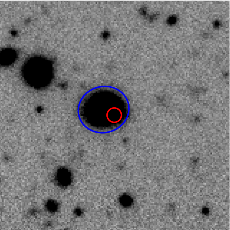
(a) CFHT image.

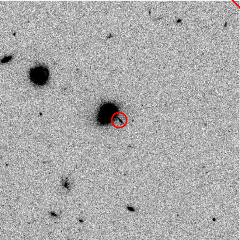
(b) HST image from the COSMOS survey

Figure 2: Images of the field around the supernova SNLS-04D2kr at $z=0.744$. The images span 30″and are oriented north-up/east-left. A red circle indicates the supernova position. A blue ellipse indicates the closest galaxy, as detected on the CFHT image.

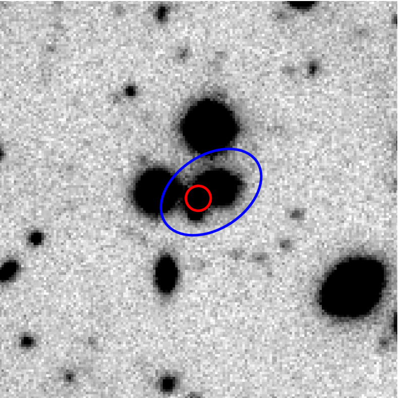
(a) CFHT image

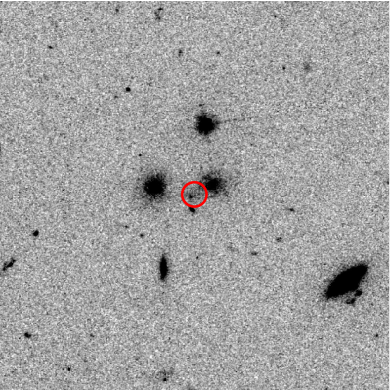
(b) HST image from the COSMOS survey

Figure 3: Field around SNLS-05D2bt at $z=0.68$. As for SNLS-04D2kr, a smaller and fainter galaxy is conspicuous on the SN location on the HST image.

We obtain in this way a photometric catalog in the $ugriz$ bands, where stars and supernovae host galaxies are identified. The host galaxy magnitudes are free from supernova light.

4.1.1 Masks

Halos and diffraction spikes around bright stars generate spurious galaxy detections in the catalog. The size of the halos and the shape of the spikes are fixed by the geometry of the telescope optics, but their intensity in the images is directly proportional to the brightness of the stars. Also, for the brightest stars, pixels reaching their saturation level induce bleedings in the CCD images which have to be accounted for.

Due to those effects, circles with radius varying from 50 to 600 pixels (10 to 120″) centered around bright stars are masked out. Those masked regions represent 22% of the field of view. An example is displayed in Figure 4 for the D1 field.

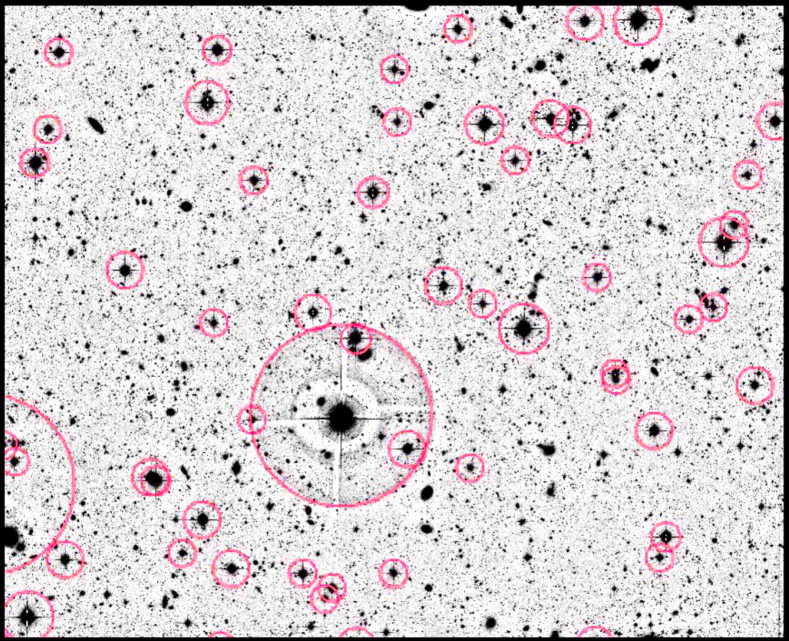
Figure 4: A section of the D1 field (5000x4500 pixels or 15.4x13.9′) with the masked areas shown as purple circles.

For each supernova we have included galaxies within a radius of 60″(see $\S$4.4). This will be referred to as the selected area. In theory, one should exclude all SNe where the selected area overlap a masked area, but this means rejecting about half of the SNe. However, the effect on the magnification of small spurious galaxies or diffraction spikes in the outskirts of the selected area is small and we chose to keep all SNe with an angular separation larger than 40″of masked areas. This leads to the exclusion of 53 SNe.

All SNe have also been looked at by eye to see whether there are other effects that could lead to exclusion, e.g. non-masked stars very close to the line of sight leading to the possibility of excluding an important galaxy hidden behind the star or leading to possible bad photometry for the surrounding galaxies. Looking at the SNe we exclude 9 of them and as a conclusion we keep 171 SNe out of 233 in the initial sample.

4.2 Photometric redshifts

High quality photometric redshifts have been published by Ilbert et al. (2006) for the galaxies in the SNLS fields down to $i_{\rm AB}\simeq 24$. In these catalogs, fluxes of galaxies hosting supernovae are affected by the supernovae light, leading sometimes to unreliable typing and redshift for these galaxies. We also need the SED used to derive the photometric redshift, so as to compute the restframe magnitudes. Finally, we need to be able to propagate easily the uncertainties of the photometric measurements to the photo-z and the absolute magnitude estimations. For these reasons, and so as to control the error propagation path, we have chosen to derive the photometric redshifts and the absolute magnitudes as follows.

We first define a continuous one parameter ($a_{*}$) galaxy spectral sequence, $F(a_{*},\lambda)$. Indeed as we have two other parameters to estimate (magnitude and redshift), we cannot afford more than a single parameter to index the diversity of galaxies in order to keep one constraint, when, even though 5 bands are used, only 4 are well measured ($griz$, $u$ being significantly shallower) . To define this spectral template, we use the galaxy evolution model PEGASE.2 (Fioc & Rocca-Volmerange, 1999), using a variety of galaxy SFR law $\propto(t/\tau)\times\exp(-t/\tau)$ and galaxy ages. The initially zero gas metallicity evolves through the successive generations of stars and ranges from $Z\!\sim\!0.$ to $0.03$. Extinction is computed using a transfer model for an inclination-averaged disk distribution, the optical depth being estimated from the mass of gas and the metallicity. We left aside the possibility to add an additional extinction.

The next step consists in optimizing the spectral sequence so as to reproduce the observed colors of our data in the best way.

It can be corrected to about 30 %, so that the final template spectra do differ from the initial computed template : our technique is thus marginally sensitive to the input model. The training set comprises a sample of galaxies with known spectroscopic redshift from the DEEP2 survey (Davis et al., 2003, 2007). The spectral sequence consists in the galaxy flux as a function of wavelength and the age index, and we optimize a multiplicative correction (a smooth function of wavelength and age index), along with offsets to the photometric zero points (which can be interpreted as differential aperture corrections). We find a residual scatter of 0.097, 0.015, 0.035, 0.025, 0.050 mag for $ugriz$ bands respectively.

The performance of the photometric redshift computation is evaluated using VVDS spectroscopic redshifts available for the D1 field (3595 galaxies at $0.01<z<1.5$) (Le Fèvre et al., 2004). The redshift residuals (i.e. $\Delta$z=photometric redshift - spectroscopic redshift) as a function of spectroscopic redshift are shown in Figure 5. For $i_{\rm AB}<24$, the fraction of catastrophic failures for which $\Delta z/(1+z)>0.15$ is $6\%$. Eliminating catastrophic failures, we obtain $\sigma_{\Delta z}=0.065$ and $\sigma_{\Delta z/(1+z)}=0.037$. Note that we do not apply any prior on the photometric redshift,

as a large fraction of the SNLS galaxies are much fainter than those of the training set.

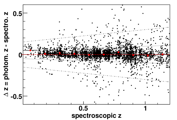
Figure 5: Performance of the photometric redshift determination: the difference $\Delta z$ between spectroscopic and photometric redshift as a function of spectroscopic redshift. The spectroscopic redshifts were obtained from the VVDS survey (Le Fèvre et al., 2004).

Uncertainties are estimated using a Monte Carlo propagation of magnitude uncertainties accounting for the measurement uncertainties and the residual scatter obtained from the training procedure. In Figure 6 we compare the scatter of $\Delta z$ for the VVDS test sample to the uncertainty on the photometric redshift derived from the Monte Carlo propagation. Both are in reasonable agreement which validates our method for propagating uncertainties.

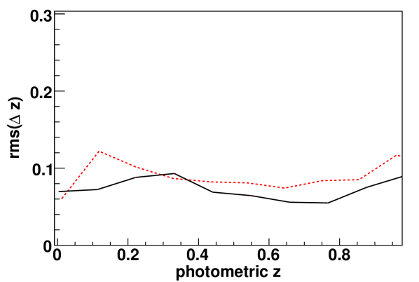
Figure 6: Performance of our photometric redshift determination: the uncertainty in the estimated photo-z using the spectroscopic VVDS redshift as a function of photo-z (in dotted red) and the photo-z uncertainty (solid black line)

For some of the galaxies it has been possible to obtain spectroscopic redshifts from VVDS, DEEP-2 and the SNLS spectroscopic program on VLT (some field galaxies were targeted at the same time as the SN primary target during observations with FORS-2 in multi-slit mode). The D2 field overlaps with the COSMOS field and it has thus been possible to use high resolution photometric redshifts for a large fraction of the galaxies in the D2 field (Ilbert et al., 2009).

4.3 Classification of spiral and elliptical galaxies based on their colors

The Tully-Fisher and Faber-Jackson relations are derived for spiral galaxies and elliptical galaxies respectively and as a consequence it is necessary to separate the SNLS galaxies into spirals and ellipticals. Note that this classification is not strictly necessary: we could blindly apply some sort of average mass-luminosity relation to all galaxies. There is indeed no typing involved in our analysis based on galaxy-galaxy lensing mass estimates. Separating in broad types is not more than a way to a priori improve the significance of a potential detection.

The SNLS imaging data does not permit a good morphological classification and we resorted to using a simple color cut to classify our galaxies. The rest-frame color $U\!-\!V$ is computed giving rise to two well separated distributions (the red and the blue population). In Figure 7 the rest-frame color $U\!-\!V$ for the SNLS galaxies is shown. For $U\!-\!V>0.54$, the galaxy is classified as an elliptical galaxy or else it is classified as a spiral galaxy. Using the rest-frame $U\!-\!V$ color as a proxy for galaxy classification is obviously not optimal, and the effect of miss-classifying the galaxies will degrade the lensing signal (see $\S$5.3.3).

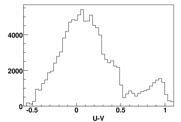
Figure 7: Distribution of the rest-frame $U\!-\!V$ color for the SNLS galaxies. A cut at $U\!-\!V=0.54$ separates the distribution into red (elliptical) and blue (spiral) galaxies.

To evaluate whether this cut provides a good estimate for galaxy typing we compare our galaxy types to those published in Ilbert et al. (2006) and Ilbert et al. (2009). They correspond to the galaxy template type, as fitted with eventually some additional extinction, using respectively 5 and 30 band magnitude measurements. For $i_{\rm AB}\leqslant 24$, we have classified $89.5\%$ of the COSMOS and $95.3\%$ of the CFHTLS elliptical galaxies as ellipticals. However $56.8\%$ and $26.9\%$ of our elliptical galaxies are classified as spiral galaxies in the COSMOS and the CFHTLS respectively, with an additional extinction of $<E(B\!-\!V)>\simeq 0.2$. In conclusion, we identify mainly all elliptical galaxies, but there is a contamination of our color-selected elliptical sample with red extinct spiral galaxies. This contamination will dilute the lensing signal : the red spirals misidentified as ellipticals will be attributed too high a mass, falsely increasing the supernova expected gravitational magnification, and thus decreasing its correlation with Hubble diagram residuals.

4.4 Gravitational magnification

The density profile of a SIS can be written

$$\rho_{\rm SIS}(r)=\frac{\sigma^{2}}{2\pi r^{2}}$$ (4)

The total mass of the halo, $m(r)=2\sigma^{2}r$, diverges and as a consequence we can use a truncation radius, $r_{t}$ to be able to estimate the total mass of the halo. The truncation radius is chosen to be $r_{200}=\sqrt{2}\sigma/10\,H(z)$ which is defined as the radius within which the mean mass density is 200 times the critical density. In this case, the convergence is given by

$$\kappa_{\rm SIS}(\theta)=\frac{\theta_{E}}{\pi\theta}\arctan\sqrt{\frac{r_{200}^{2}}{\theta^{2}D_{l}^{2}}-1}$$ (5)

in the thin lens approximation, where $\theta$ is the transverse angle of the image to the lens, and $\theta_{E}=4\pi(\sigma/c)^{2}D_{ls}/D_{s}$ is the Einstein radius. $D_{ls}$, $D_{s}$ and $D_{l}$ are respectively the angular distances from the lens to the source, from the observer to the source and from the observer to the lens, and $\sigma$ is the velocity dispersion. In order to compute the magnification due to several galaxy lenses, we use the publicly available software Q-LET (Gunnarsson, 2004), which uses the multiple lens plane method.

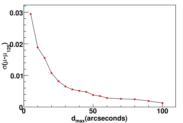
Figure 8: r.m.s of the difference of magnifications $\mu(d_{\rm max})-\mu(d_{\rm max}=125\arcsec)$ as a function of $d_{\rm max}$. This simulation (from real lines of sight) is done for a source at a redshift of 1.

We have investigated the effect on the estimated magnification of truncating the galaxy list around lines of sight. We have considered for this purpose random lines of sight in the galaxy catalog, and computed for each of them the magnification for a SN at $z=1$, considering sequentially an increasing number of galaxies in the foreground according to their (transverse) angle $\theta$ to the SN. Figure 8 displays the r.m.s of the difference of magnifications $\mu(d_{\rm max}<125\arcsec)-\mu(d_{\rm max}=125\arcsec)$ as a function of $d_{\rm max}$, where $d_{\rm max}$ is the maximum transverse angle of galaxies used to compute the magnification. For $d_{\rm max}=60\arcsec$, the average error on the estimated magnification due to this galaxy selection is of 0.003. This number is much smaller than the other sources of uncertainties so that we can safely ignore galaxies at larger angles.

4.4.1 Normalization of the magnification distribution

To estimate the magnification using Q-LET, the lensing galaxies have been put on top of a homogeneously distributed universe leading to computed gravitational magnifications always greater than 1 compared to such a universe. As a consequence the magnifications should be normalized in order to force the average magnification to be equal to 1, as imposed by flux conservation.

For this purpose, we have considered numerous random lines of sight (randomly chosen source positions) using the true galaxy catalog for a range of source redshifts and computed the magnification for each of them. The average magnification for each redshift bin (of 0.1) is recorded and subsequently used to normalize the magnification estimates. This correction function is calculated for each field and each mass-luminosity relation.

4.4.2 Magnification uncertainty calculation

The uncertainties on the magnifications are evaluated with a Monte Carlo propagation of the magnitude uncertainties of the galaxies from the catalog and the scatter in the mass-luminosity relations.

Magnitude uncertainties include both measurement uncertainties and the residual scatter of the photometric redshift training (see $\S$4.2).

A fit of the photometric redshift is performed for each Monte Carlo realization of each galaxy, except for those which have much more precise spectroscopic or photometric redshifts from other sources. For instance, high resolution photometric redshifts are available for galaxies of the COSMOS catalog (Ilbert et al., 2009). For those, instead of fitting for the redshift, we considered random realizations of the redshift within the errors given in their paper, and used our code with those fixed redshifts to determine the uncertainties on the absolute magnitudes.

The scatter in the TF and FJ mass-luminosity relations are well defined from the observations (see $\S$2.1 and $\S$2.2). However, there is no such scatter for the mass luminosity relation derived from galaxy-galaxy lensing observations, as this relation is the result of a global fit to a halo model where each galaxy provide little information. Therefore, for this relation we assume the same scatter as for the TF relation.

In Figure 9 we show the uncertainty of the magnification as a function of the magnification obtained with the TF/FJ relations. We obtain a relative uncertainty on the magnification of 17%. The most important source of uncertainty comes from the scatter in the mass-luminosity relation. The uncertainties due to redshift are small and represent a relative uncertainty of about 5%.

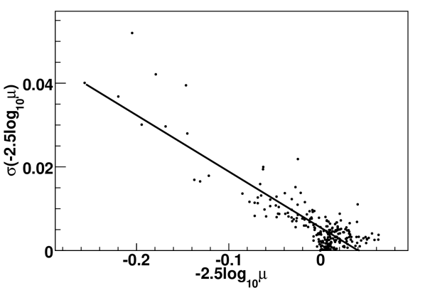
Figure 9: Magnification uncertainty as a function of magnification both expressed in magnitudes. The line is a straight line fit to the data. The relative uncertainty is about 17%.

5 Signature of the lensing effect

5.1 Signal discriminant

As a criterion for a lensing signal detection we have chosen to calculate the weighted correlation coefficient.

$$\rho=\frac{\mathit{cov}(\mu_{m},r)}{\sqrt{\mathit{var}(\mu_{m})\mathit{var}(r)}}$$ (6)

with $\mu_{m}=-2.5\log_{10}{\mu}$, $\mu$ being the gravitational magnification factor, and $r$ is the residual to the Hubble diagram (hereafter Hubble residual). The weighted covariance of two variables $x$ and $y$, can be written as :

$$\mathit{cov}(x,y)=\frac{\sum wxy}{\sum w}-\bar{x}\bar{y}$$ (7)

where $w$ is the weight assigned to each datapoint and $\bar{x}$ and $\bar{y}$ are the weighted means. Using random lines of sight (ie. random source positions in the galaxy catalog), we have found that weighting with the inverse of the Hubble residual variance is optimal for the signal detection. Note that any scaling applied to $\mu_{m}$ and hence any common offset applied to the mass-luminosity relations will not change the weighted correlation coefficient and thus not change the detection significance.

5.2 Expected Signal

Before presenting the results, it is useful to have an idea of what to expect. We now have all the tools needed to perform detailed Monte Carlo simulations using the true galaxy catalog and give precise predictions both for the SNLS 3-year data set and the full SNLS sample.

Magnification distributions for supernovae at different redshifts were generated by calculating the magnification factor for a sample of simulated supernovae randomly positioned in the true galaxy catalog. In this way it was possible to simulate the magnification distribution for a sample of supernovae with a given redshift distribution, chosen as the actual sample redshift distribution. To generate a correlated sample, i.e assuming a correlation between the Hubble residual and the magnification, we first computed a “true” magnification using the TF/FJ relations applied to galaxies along the line of sight. We then drew an expected magnification using the uncertainty described in 4.4.2. The corresponding Hubble residuals were eventually generated from the expected magnification and a random offset of r.m.s 0.16 mag in accordance with the SNLS data for which the Hubble residuals exhibit an r.m.s of 0.16 mag. An uncorrelated sample can be generated by randomly assigning a Hubble residual to each expected magnification.

We first simulated a large number of correlated samples similar to the real one with 171 supernovae. We compared the distribution of the weighted correlation coefficient of these samples with that of uncorrelated samples

(see Figure 10).

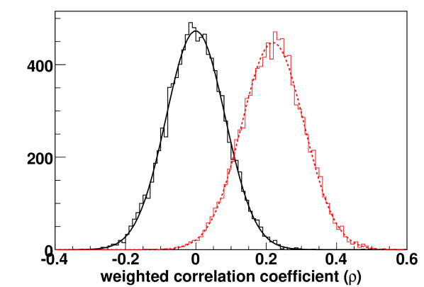
Figure 10: Simulated distribution (using real lines of sight) of the weighted correlation coefficients for correlated samples (dotted) and uncorrelated samples (solid), for the 3-year SNLS sample. There is 50 % probability of finding a 2.5 $\sigma$ significance correlation or better ($\rho=0.22$) and 35 % probability of detecting a 3 $\sigma$ signal ($\rho=0.25$).

We find that for the current sample there is 50 % probability of finding a 2.5 $\sigma$ significance correlation or better and 35 % probability of detecting a 3 $\sigma$ signal.

For the final SNLS sample we expect $\sim$400 spectroscopically confirmed Type Ia supernovae and $\sim$200 photometrically identified Type Ia supernovae. Due to masking, about a third of the supernovae will be rejected. If we do simulations for 400 supernovae with the same parameters as the current sample we find that there is 80% probability of detecting a 3 $\sigma$ signal or more (see Figure 11 ).

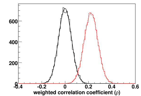
Figure 11: Same distributions as Figure 10, for the simulated full SNLS sample. There is 80% probability of detecting a 3 $\sigma$ signal ($\rho=0.22$) or better.

Another question to be addressed is how the errors influence the possibility of a signal detection. The errors on the magnification are already small. Monte Carlo simulations performed with various scaled errors of the magnification support that the scatter in the magnification has

little impact on the signal detection. The signal detection is highly dominated by the scatter in the SN Hubble residuals which is not likely to decrease significantly in the near future. As a consequence improving the signal detection will require better statistics and, if possible, higher redshift SNe.

5.3 Results

5.3.1 The SNLS supernovae

The 3-year data release contains 233 spectroscopically confirmed Type Ia supernovae in the redshift range 0.2-1.05 after quality cuts.

The Hubble residual of the supernova is the difference in distance modulus of the supernova and the best cosmology fit. The distance modulus is estimated from the supernova brightness and other parameters resulting from a fit of the SALT2 model (Guy et al., 2007) to the supernova light curves. The uncertainty of a distance modulus combines three sources: the photometric measurement uncertainties, the light curve model scatter (see Guy et al. (2007) for a detailed definition), and the so-called intrinsic scatter which expresses our lack of complete physical understanding of SN Ia. This intrinsic scatter is chosen so that the minimum $\chi^{2}$ of cosmological fits to the Hubble diagram matches the number of degrees of freedom. This ensures that the quoted uncertainties of Hubble residuals properly describe their actual scatter.

5.3.2 Magnification

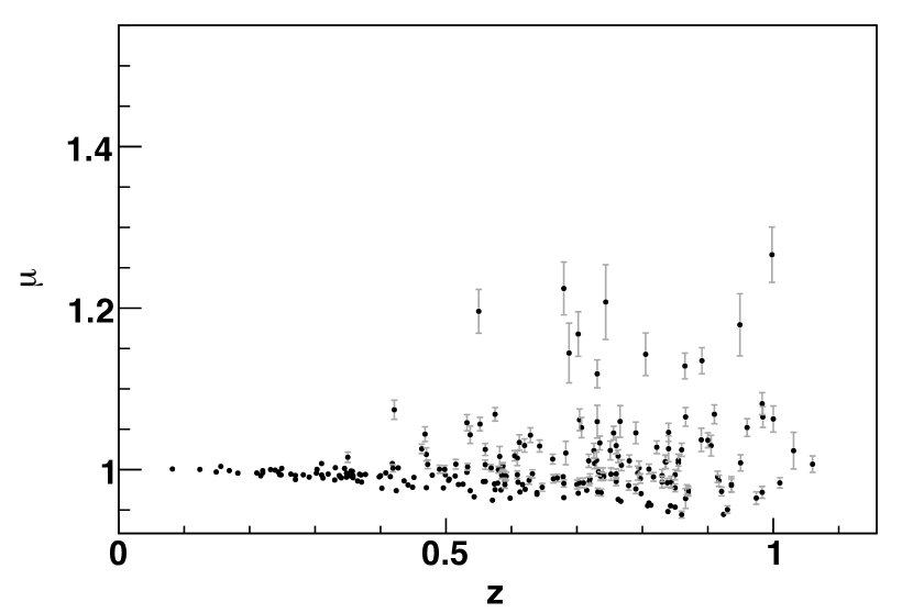
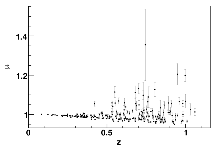
Figure 12: Magnification factor of the SNLS supernovae versus redshift. Results based on the K06 luminosity-mass relation (top) and on TF and FJ relations (bottom). Most of the SNe are slightly demagnified whereas some are significantly magnified.

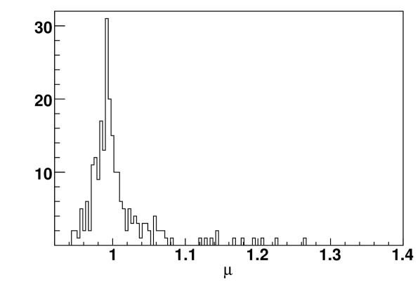
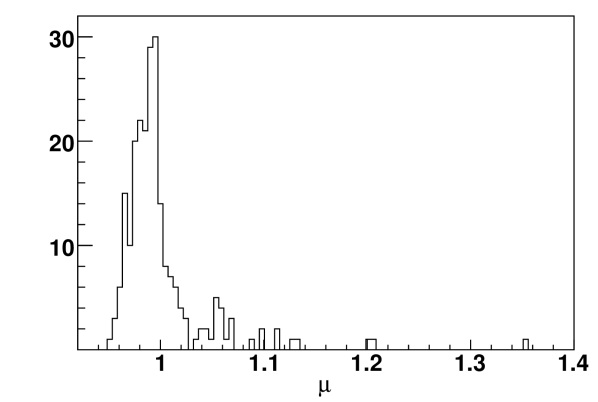
Figure 13: Magnification distribution of the SNLS supernovae. Results based on the K06 luminosity-mass relation (top) and on TF and FJ relations (bottom). The magnification distributions peaks at a value slightly below 1 and presents a high magnification tail.

		magnification factor $\mu$		Most important lensing galaxies
SN	z	K06	TF-FJ	z(galaxy)	d (″)	$\sigma$ km/s (K06)	$\sigma$ km/s (TF-FJ)
04D1iv	0.998	1.267$\pm$0.034	1.199$\pm$0.031	0.60	7.8	299	295
				0.51	5.8	217	154
04D2kr	0.744	1.208$\pm$0.046	1.355$\pm$0.182	0.228	1.5	119	150
05D2by	0.891	1.135$\pm$0.016	1.059$\pm$0.035	0.66	1.8	89	50
				0.68	4.3	151	167
				0.44	2.7	88	54
05D2bt	0.68	1.224$\pm 0.33$	1.113$\pm$0.033	0.31	0.5	99	65
05D3cx	0.805	1.143 $\pm$0.026	1.127$\pm$0.035	0.38	6.4	224	243
03D4cx	0.949	1.179$\pm$0.038	1.205$\pm$0.054	0.45	5.5	246	259
04D4bq	0.55	1.196$\pm$0.027	1.114$\pm$0.028	0.32	4.4	152	108
				0.38	4.1	190	138
05D4cq	0.702	1.168$\pm$0.028	1.133$\pm$0.026	0.28	15.7	282	298
				0.43	2.9	106	67

Table 1: The most magnified supernovae and the characteristics of the galaxies dominating the magnification.

Figure 12 and 13 show the magnification of each SN as a function of redshift and the magnification distribution respectively. As expected, most SNe are demagnified with respect to a homogeneous universe and some are significantly magnified. Moreover, the magnification distribution peaks at a value slightly lower than one and presents a long magnification tail. Images of galaxies along the line-of-sight of 3 of the most magnified supernovae (04D1iv, 03D4cx and 04D4bq) in the 3-year data set are shown in Figure 14 (see also Figure 3 & 3). All 3 SNe have one or several massive galaxies very close to the line-of-sight located roughly halfway between the SN and us, causing the high magnification. The 8 most magnified supernovae along with information on the most important galaxies causing the magnification are listed in table 1.

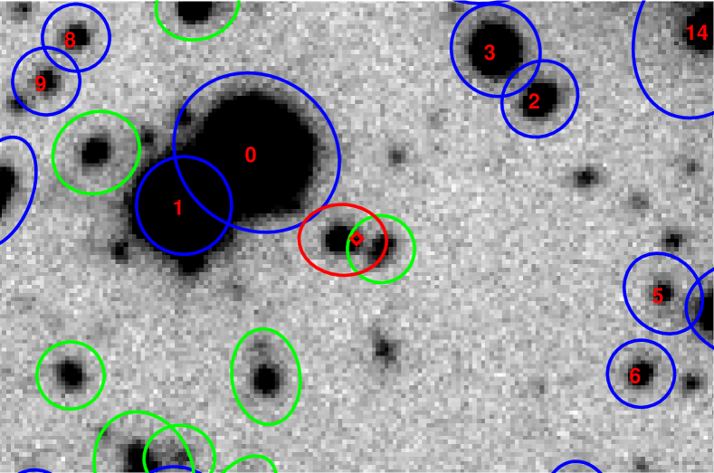
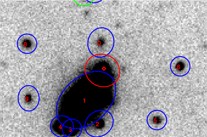
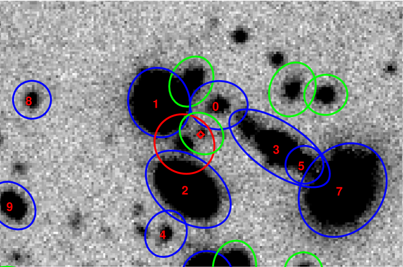
Figure 14: From the top to the bottom, SN 04D1iv at a redshift of 0.998, SN 03D4cx at a redshift of 0.949 and SN 04D4bq at a redshift of 0.550. In red, the SN and its host. In blue the foreground galaxies labeled according to the closest elliptical distance to the SN and in green the background galaxies. All images span 30″(horizontally) and are oriented north-up/east-left.

5.3.3 Correlation

We are searching for a correlation between the Hubble residuals from a best fit cosmological model and the estimated magnifications of the supernovae based on foreground galaxy modeling. In Figure 15 we show a plot of the Hubble residuals of the 171 SNe versus the estimated magnification.

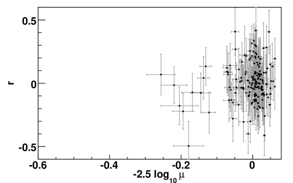
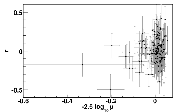
Figure 15: The Hubble residuals as a function of magnification for the SNLS. Results based on the K06 luminosity-mass relations (top) and on TF and FJ relations (bottom).

The weighted correlation coefficient for this sample is $\rho=0.12$ using the K06 relation and $\rho=0.18$ using the TF and FJ relations respectively. To evaluate the strength of the correlation we calculate the distribution of the weighted correlation coefficient for an uncorrelated sample and compare it with the obtained value for our sample (see Figure 16). The uncorrelated samples are drawn by randomly associating Hubble residuals and expected magnifications of the real sample. The probability of finding a larger weighted correlation coefficient than the measured one from an uncorrelated sample is 5% using the K06 relation and 1% using the TF and FJ relations, corresponding to 1.6 and $2.3\,\sigma$ detections respectively.

It is tempting to attribute the stronger detection of the TF/FJ relation to the fact that this method considers separately elliptical and spiral galaxies. In order to test the influence of the separation, we run the analysis again, but with a random galaxy type assignment (however preserving the measured proportions). We then find that the significance of the detection drops from 2.3 to 1.4 $\sigma$, and conclude that the higher significance of our detection using TF/FJ relations can be attributed to the distinction between spiral and elliptical galaxies, rather than chance. So, our primary result is the detection of supernovae lensing using TF/FJ relations at the 99% CL. Note that simulations assuming a perfect galaxy typing (see section 5.2) give rise to a mean detection level of 2.5 $\sigma$ (see Figure 10). The 2.3 $\sigma$ detection we find is thus close to the optimal so that further improvements on galaxy typing should not give rise to a much larger significance of the signal.

In order to test the scale of galaxy mass estimates, we fit the slope $a$ relating Hubble residuals and expected magnifications : $<r>=a<\mu_{m}>$ and find $a=0.65\leavevmode\nobreak\ \pm\leavevmode\nobreak\ 0.30$. Hence the data are consistent with the TF/FJ mass-luminosity relations at the 1.2 $\sigma$ level, with a precision of 30%.

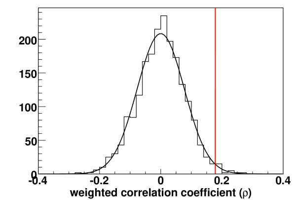
Figure 16: Distribution of the weighted correlation coefficient for an uncorrelated sample when using TF and FJ relations (in black). The red line indicates the value $\rho=0.18$ obtained for our sample. The measured correlation significance is $2.3\,\sigma$ (99% CL).

Using random lines of sight in the real data, we can estimate the increase of Hubble diagram scatter expected from gravitational lensing, as a function of redshift. This is shown in Figure 17 for the TF/FJ relations, which can be roughly described as $\sigma(\mu_{m})=0.08\times z$. Alternatively, if we use the value of $a$ derived from a fit of the relation between Hubble residuals and magnifications, we obtain a lower value $\sigma(\mu_{m})=(0.05\pm 0.022)\times z$.

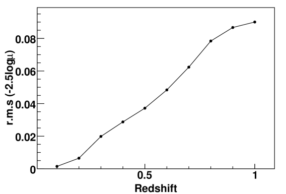
Figure 17: Expected magnification scatter from random lines of sight as a function of the source redshift, using the TF/FJ mass-luminosity relations.

6 Conclusion

We have calculated the expected magnification of the SNLS 3-year sample from the foreground galaxy properties and searched for a correlation with residuals from the Hubble diagram. A correlation is detected at the 99% CL, compatible with a slope of 1.

The expected magnifications cause an extra scatter in the Hubble diagram approximated by $0.08\times z$ from the TF/FJ relations we used, which becomes $(0.05\pm 0.022)\times z$ once these TF/FJ relations are calibrated with the supernova data. We show that separating the galaxy sample into a blue and a red population based on a $U\!-\!V$ color cut increases the significance of the detection. This is due to the fact that the mass estimate and hence the induced magnification is significantly different for a red and a blue galaxy of same luminosity (the TF and FJ relations). Simulations also point to the fact that a signal detection is dominated by the number of SNe, their redshift distribution and the scatter in the SN residuals. Reducing the scatter in the estimated magnification by increasing the photometric redshift precision or reducing the scatter in the TF and FJ relations have little effect on the probability of a signal detection.

Finally, simulations using the true galaxy catalog show that using the full SNLS data set ($\sim$400 expected spectroscopically confirmed Type Ia SNe and $\sim$200 photometrically identified Type Ia SNe) there is 80% chance of detecting a $3\,\sigma$ signal or more.